


1. Introduction
As one of the most famous integrable equations in physics, the nonlinear Schrödinger (NLS) equation can be reduced from the AKNS system [1]. It is natural to propose several generic deformations of the NLS equation under higher-order perturbations. Among them, there are three kinds of the derivative nonlinear Schrödinger (DNLS) equations. They are regarded as having important roles in various fields of mathematical physics such as nonlinear water waves, plasma astrophysics, and nonlinear optics fibers [2, 3]. One version of the celebrated DNLS equation is presented in the form
$\begin{eqnarray}{\rm{i}}{q}_{t}+{q}_{{xx}}+{\rm{i}}\varepsilon {q}^{2}{q}_{x}^{* }+\displaystyle \frac{1}{2}{q}^{3}{q}^{* 2}=0,\end{eqnarray}$
where the sign * denotes the complex conjugation and ϵ = ±1. It is also known as the DNLS-III or GI equation which is reduced from the coupled GI equation [4] by a reduction.As a generalization of an integrable system of NLS type, the GI equation has been studied from various points of views in [5–12]. A bi-Hamiltonian structure and Liouville integrability for GI hierarchy were proposed in [13]. The Lax pair and exact solutions of equation (1 ) were obtained in [14–16] via the Darboux transformation (DT). [17] provided the determinant expression of higher-order solutions including higher-order rational solutions and higher-order rogue wave solutions. We note that the GI equation (1 ) was investigated by bifurcation theory and the existence of travelling wave solutions was verified [18]. In [19], the authors sought the exact solutions with trigonometric and rational functions with the aid of exp-expansion method. The sine-Gordon equation approach and Riemann-Hilbert method were carried out to the GI equation [20, 21].
Recently, many researchers have focused on the ${ \mathcal P }{ \mathcal T }$-symmetric phenomena, and the theory of ${ \mathcal P }{ \mathcal T }$-symmetry is applied to nonlinear integrable systems in mathematical physics [22–24]. Some nonlocal equations have been presented successively soon after Ablowitz and Musslimani initially introduced the nonlocal NLS equation and derived its solutions by the inverse scattering transformation [25]. Particular examples are the nonlocal KP equation, the nonlocal mKdV equation, the nonlocal DS equations, the nonlocal Boussinesq equation, and so on. These nonlocal cases are obviously different from local integrable equations, which arouse renewed interest in nonlinear integrable systems. The DT has been attested to be an efficient algorithm in many circumstances to obtain soliton, breather, and rogue wave solutions of nonlinear integrable equations [26–29]. Several nonlocal systems have been proposed and studied by using DT [30–34].
In this work, we investigate the integrable nonlinear coupled GI equation
$\begin{eqnarray}{\rm{i}}{q}_{t}+{q}_{{xx}}+{\rm{i}}{q}^{2}{r}_{x}+\displaystyle \frac{1}{2}{q}^{3}{r}^{2}=0,\end{eqnarray}$
$\begin{eqnarray}{\rm{i}}{r}_{t}-{r}_{{xx}}+{\rm{i}}{r}^{2}{q}_{x}-\displaystyle \frac{1}{2}{q}^{2}{r}^{3}=0,\end{eqnarray}$
which can be derived through a zero-curvature equation. It leads to the nonlocal GI equation $\begin{eqnarray}{\rm{i}}{q}_{t}+{q}_{{xx}}+{\rm{i}}\varepsilon {q}^{2}{q}_{x}(-x,-t)+\frac{1}{2}{q}^{3}{q}^{2}(-x,-t)=0,\end{eqnarray}$
by the reduction q(x, t) = ϵ r(−x, −t), then take the case ϵ = −1.This paper is organized as follows. In section 2 , the DT of equation (3 ) is discussed based on the presented Lax pair. In section 3 , we obtain different kinds of solutions including bright-dark soliton, periodic, rogue wave, W-shaped soliton and kink solutions from zero and nonzero seed solutions. The conclusions are given in section 4 .
2. The Lax pair and Darboux transformation
In this section, we consider the Lax pair of a coupled GI equation (2 )
$\begin{eqnarray}{{\rm{\Phi }}}_{x}=U(x,t,\lambda ){\rm{\Phi }},\end{eqnarray}$
$\begin{eqnarray}{{\rm{\Phi }}}_{t}=V(x,t,\lambda ){\rm{\Phi }},\end{eqnarray}$
where $\begin{eqnarray}\begin{array}{rcl}U & = & \left(\begin{array}{cc}-{\rm{i}}{\lambda }^{2}-\displaystyle \frac{1}{2}{\rm{i}}{qr} & \lambda q\\ \lambda r & {\rm{i}}{\lambda }^{2}+\displaystyle \frac{1}{2}{\rm{i}}{qr}\end{array}\right),\\ V & = & \left(\begin{array}{cc}A & B\\ C & -A\end{array}\right),\end{array}\end{eqnarray}$
with $\begin{eqnarray}\begin{array}{rcl}A & = & -2{\rm{i}}{\lambda }^{4}-{\rm{i}}{qr}{\lambda }^{2}+\displaystyle \frac{1}{2}({{rq}}_{x}-{{qr}}_{x})+\displaystyle \frac{1}{4}{\rm{i}}{q}^{2}{r}^{2},\\ B & = & 2q{\lambda }^{3}+{\rm{i}}{q}_{x}\lambda ,\quad C=2r{\lambda }^{3}-{\rm{i}}{r}_{x}\lambda .\end{array}\end{eqnarray}$
Firstly, we introduce the following gauge transformation4 ) is transformed into4 ) at λ = λ1. Similarly, considering the eigenfunctions ${{\rm{\Phi }}}_{i}\,={({\phi }_{i},{\varphi }_{i})}^{T},(i=1,2,\cdots ,n)$, the N-fold DT can be expressed by the same process and the transformations between $\left({q}^{[n]},{r}^{[n]}\right)$ and $\left({q}^{[0]},{r}^{[0]}\right)$ are
$\begin{eqnarray}{{\rm{\Phi }}}^{[1]}={{\rm{T}}}^{[1]}{\rm{\Phi }},\end{eqnarray}$
and it is easy to see that the spectral problem ( $\begin{eqnarray}{{\rm{\Phi }}}_{x}^{[1]}={({{\rm{T}}}_{x}^{[1]}+{{\rm{T}}}^{[1]}U)({{\rm{T}}}^{[1]})}^{-1}{{\rm{\Phi }}}_{1}\triangleq {U}^{[1]}{{\rm{\Phi }}}_{1},\end{eqnarray}$
$\begin{eqnarray}{{\rm{\Phi }}}_{t}^{[1]}={({{\rm{T}}}_{t}^{[1]}+{{\rm{T}}}^{[1]}V)({{\rm{T}}}^{[1]})}^{-1}{{\rm{\Phi }}}_{1}\triangleq {V}^{[1]}{{\rm{\Phi }}}_{1}.\end{eqnarray}$
Based on DT in [15], the Darboux matrix T can be established as $\begin{eqnarray}{\rm{T}}(\lambda )=\left(\begin{array}{cc}\lambda & {b}_{1}\\ {c}_{1} & \lambda \end{array}\right),\end{eqnarray}$
where b1, c1 are all functions of x and t. Then on comparing the identical power of λ and using the fact of T[1]Φ1 = 0, 1-fold DT is obtained, where Φ1 is a nonzero solution of ( $\begin{eqnarray}\begin{array}{rcl}{q}^{[n]} & = & {q}^{[0]}+2{\rm{i}}{b}_{n}={q}^{[0]}+2{\rm{i}}\displaystyle \frac{{\delta }_{11}}{{\delta }_{12}},\\ {r}^{[n]} & = & {r}^{[0]}-2{\rm{i}}{c}_{n}={r}^{[0]}-2{\rm{i}}\displaystyle \frac{{\delta }_{21}}{{\delta }_{22}},\end{array}\end{eqnarray}$
where, for N = 2n, $\begin{eqnarray*}\begin{array}{rcl}{\delta }_{11} & = & \left|\begin{array}{ccccc}{\phi }_{1} & {\lambda }_{1}{\varphi }_{1} & \cdots & {\lambda }_{1}^{n-2}{\phi }_{1} & -{\lambda }_{1}^{n}{\phi }_{1}\\ {\phi }_{2} & {\lambda }_{2}{\varphi }_{2} & \cdots & {\lambda }_{2}^{n-2}{\phi }_{2} & -{\lambda }_{2}^{n}{\phi }_{2}\\ \vdots & \vdots & \vdots & \vdots & \vdots \\ {\phi }_{n} & {\lambda }_{n}{\varphi }_{n} & \cdots & {\lambda }_{n}^{n-2}{\phi }_{n} & -{\lambda }_{n}^{n}{\phi }_{n}\end{array}\right|,\\ {\delta }_{12} & = & \left|\begin{array}{ccccc}{\phi }_{1} & {\lambda }_{1}{\varphi }_{1} & \cdots & {\lambda }_{1}^{n-2}{\phi }_{1} & {\lambda }_{1}^{n-1}{\varphi }_{1}\\ {\phi }_{2} & {\lambda }_{2}{\varphi }_{2} & \cdots & {\lambda }_{2}^{n-2}{\phi }_{2} & {\lambda }_{2}^{n-1}{\varphi }_{2}\\ \vdots & \vdots & \vdots & \vdots & \vdots \\ {\phi }_{n} & {\lambda }_{n}{\varphi }_{n} & \cdots & {\lambda }_{n}^{n-2}{\phi }_{n} & {\lambda }_{n}^{n-1}{\varphi }_{n}\end{array}\right|,\end{array}\end{eqnarray*}$
$\begin{eqnarray*}\begin{array}{rcl}{\delta }_{21} & = & \left|\begin{array}{ccccc}{\varphi }_{1} & {\lambda }_{1}{\phi }_{1} & \cdots & {\lambda }_{1}^{n-2}{\varphi }_{1} & -{\lambda }_{1}^{n}{\varphi }_{1}\\ {\varphi }_{2} & {\lambda }_{2}{\phi }_{2} & \cdots & {\lambda }_{2}^{n-2}{\varphi }_{2} & -{\lambda }_{2}^{n}{\varphi }_{2}\\ \vdots & \vdots & \vdots & \vdots & \vdots \\ {\varphi }_{n} & {\lambda }_{n}{\phi }_{n} & \cdots & {\lambda }_{n}^{n-2}{\varphi }_{n} & -{\lambda }_{n}^{n}{\varphi }_{n}\end{array}\right|,\\ {\delta }_{22} & = & \left|\begin{array}{ccccc}{\varphi }_{1} & {\lambda }_{1}{\phi }_{1} & \cdots & {\lambda }_{1}^{n-2}{\varphi }_{1} & {\lambda }_{1}^{n-1}{\phi }_{1}\\ {\varphi }_{2} & {\lambda }_{2}{\phi }_{2} & \cdots & {\lambda }_{2}^{n-2}{\varphi }_{2} & {\lambda }_{2}^{n-1}{\phi }_{2}\\ \vdots & \vdots & \vdots & \vdots & \vdots \\ {\varphi }_{n} & {\lambda }_{n}{\phi }_{n} & \cdots & {\lambda }_{n}^{n-2}{\varphi }_{n} & {\lambda }_{n}^{n-1}{\phi }_{n}\end{array}\right|.\end{array}\end{eqnarray*}$
Under the nonlocal reduction condition q(x, t) = −r(−x, −t), we have to choose the eigenfunction Φk as
$\begin{eqnarray}{\phi }_{k}(x,t)={\varphi }_{k}(-x,-t).\end{eqnarray}$
In a word, we should pay more attention to the effects of different reductions when considering the nonlocal equations.3. Exact solutions of equation (3 )
In the following contents, we select several zero and nonzero seed solutions to solve the nonlocal GI equation (3 ). With the substitution of seed solutions, we can obtain the solutions of the Lax pair for different cases.
3.1. Soliton solutions from the zero seed solution
First of all, we select trivial solution q[0](x, t) = −r[0](−x, −t) = 0, the corresponding eigenfunctions for equation (3 ) are given by
$\begin{eqnarray}{{\rm{\Phi }}}_{k}=\left(\begin{array}{c}{\phi }_{k}\\ {\varphi }_{k}\end{array}\right)=\left(\begin{array}{c}{{\rm{e}}}^{-{\rm{i}}{\theta }_{k}}\\ {{\rm{e}}}^{{\rm{i}}{\theta }_{k}}\end{array}\right),\end{eqnarray}$
where ${\theta }_{k}={\lambda }_{k}^{2}x+2{\lambda }_{k}^{4}t$.3.1.1. Soliton solutions from the zero seed solution by two-fold DT
It is easy to describe different solutions by adjusting the appropriate parameters λk (k = 1, 2). Then we get the following solution
$\begin{eqnarray}{q}^{[2]}=2{\rm{i}}\displaystyle \frac{{\phi }_{1}{\phi }_{2}({\lambda }_{1}^{2}-{\lambda }_{2}^{2})}{{\lambda }_{2}{\phi }_{1}{\varphi }_{2}-{\lambda }_{1}{\varphi }_{1}{\phi }_{2}}.\end{eqnarray}$
Case 1: Bright soliton solution
Let ${\lambda }_{1}={\lambda }_{2}^{* }$, we can gain the typical bright soliton solution
$\begin{eqnarray}{q}^{[2]}=2{\rm{i}}\displaystyle \frac{({\lambda }_{1}^{2}-{\lambda }_{1}^{* 2}){{\rm{e}}}^{-{\rm{i}}({\theta }_{1}+{\theta }_{2})}}{{\lambda }_{1}^{* }{{\rm{e}}}^{-{\rm{i}}({\theta }_{1}-{\theta }_{2})}-{\lambda }_{1}{{\rm{e}}}^{{\rm{i}}({\theta }_{1}-{\theta }_{2})}},\end{eqnarray}$
with appropriate parameters.Case 2: Kink solution
Additionally, to get another solution which is different from the one of classical GI equation, setting Re(λ2) = 0, the kink solution is derived. It follows from this solution that if Re(λ1) > 0, the form of the solution is expressed as the kink solution, and the solution given by the Re(λ1) < 0 is expressed as the anti-kink solution.
Case 3: Periodic solution
Without loss of any generality, setting Im(λ1) = Im(λ2) = 0, and the solution turns to a periodic solution,
$\begin{eqnarray}\begin{array}{l}{q}^{[2]}=2{\rm{i}}\left({\lambda }_{1{\rm{R}}}^{2}-{\lambda }_{2{\rm{R}}}^{2}\right)\\ \ \times \ \displaystyle \frac{\cos ({H}_{1})-\mathrm{isin}({H}_{1})}{({\lambda }_{2{\rm{R}}}-{\lambda }_{1{\rm{R}}})\cos ({H}_{2})-{\rm{i}}({\lambda }_{2{\rm{R}}}+{\lambda }_{1{\rm{R}}})\sin ({H}_{2})},\end{array}\end{eqnarray}$
where $\begin{eqnarray*}\begin{array}{rcl}{H}_{1} & = & \left({\lambda }_{1{\rm{R}}}^{2}+{\lambda }_{2{\rm{R}}}^{2}\right)x+2\left({\lambda }_{1{\rm{R}}}^{4}+{\lambda }_{2{\rm{R}}}^{4}\right)t,\\ {H}_{2} & = & \left({\lambda }_{1{\rm{R}}}^{2}-{\lambda }_{2{\rm{R}}}^{2}\right)x+2\left({\lambda }_{1{\rm{R}}}^{4}-{\lambda }_{2{\rm{R}}}^{4}\right)t.\end{array}\end{eqnarray*}$
Thus, the period of this solution can be obtained by direct calculation. The periodicity of the solution appears concurrently in x and t.3.1.2. Soliton solutions from zero seed solution by four-fold DT
Meanwhile, we can construct four-fold DT to get different kinds of interactional solutions with the distinct choices of parameters. Taking the same procedure as above, one can find soliton solutions of the nonlocal GI equation
$\begin{eqnarray}{q}^{[4]}=2{\rm{i}}\displaystyle \frac{{Q}_{4}}{{R}_{4}}\end{eqnarray}$
with $\begin{eqnarray*}\begin{array}{rcl}{Q}_{4} & = & \left|\begin{array}{cccc}{\phi }_{1} & {\lambda }_{1}{\varphi }_{1} & {\lambda }_{1}^{2}{\phi }_{1} & -{\lambda }_{1}^{4}{\phi }_{1}\\ {\phi }_{2} & {\lambda }_{2}{\varphi }_{2} & {\lambda }_{2}^{2}{\phi }_{2} & -{\lambda }_{2}^{4}{\phi }_{2}\\ {\phi }_{3} & {\lambda }_{3}{\varphi }_{3} & {\lambda }_{3}^{2}{\phi }_{3} & -{\lambda }_{3}^{4}{\phi }_{3}\\ {\phi }_{4} & {\lambda }_{4}{\varphi }_{4} & {\lambda }_{4}^{2}{\phi }_{4} & -{\lambda }_{4}^{4}{\phi }_{4}\end{array}\right|,\\ {R}_{4} & = & \left|\begin{array}{cccc}{\phi }_{1} & {\lambda }_{1}{\varphi }_{1} & {\lambda }_{1}^{2}{\phi }_{1} & {\lambda }_{1}^{3}{\varphi }_{1}\\ {\phi }_{2} & {\lambda }_{2}{\varphi }_{2} & {\lambda }_{2}^{2}{\phi }_{2} & {\lambda }_{2}^{3}{\varphi }_{2}\\ {\phi }_{3} & {\lambda }_{3}{\varphi }_{3} & {\lambda }_{3}^{2}{\phi }_{3} & {\lambda }_{3}^{3}{\varphi }_{3}\\ {\phi }_{4} & {\lambda }_{4}{\varphi }_{4} & {\lambda }_{4}^{2}{\phi }_{4} & {\lambda }_{4}^{3}{\varphi }_{4}\end{array}\right|.\end{array}\end{eqnarray*}$
Case 4: Two-bright soliton solution
While for ${\lambda }_{1}={\lambda }_{2}^{* }$, ${\lambda }_{3}={\lambda }_{4}^{* }$, two-bright soliton solution is easy to obtain, which is shown in figure 1.
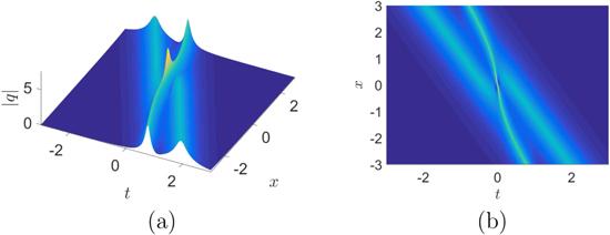
Figure 1. Two-bright soliton solution with λ1 = ${\lambda }_{2}^{* }=1.1+0.6{\rm{i}}$, λ3 = ${\lambda }_{4}^{* }=0.8+0.4{\rm{i}}$. |
Case 5: Mixed periodic solution
As shown in figure 2, to construct a mixed periodic solution, we take the parameters as ${\lambda }_{1}={\lambda }_{2}^{* }$, Im(λ3) = 0, Re(λ4) = 0. It is observed that this solution on the periodic wave background has the similar property as (15 ).
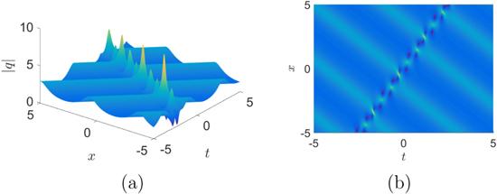
Figure 2. Mixed periodic solution with ${\lambda }_{1}={\lambda }_{2}^{* }=0.7+{\rm{i}}$, ${\lambda }_{3}$ = −0.8, ${\lambda }_{4}=0.3{\rm{i}}$. |
Case 6: Mixed kink and soliton solution
As discussed above, we can obtain different kinds of hybrid solutions with other parameter choices. In this case, for the following parameters, the mixed kink and soliton solution is shown in figure 3.
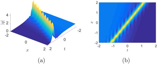
Figure 3. Mixed kink and soliton solution with λ1 = 0.2 + i, λ2 = −i, ${\lambda }_{3}={\lambda }_{4}^{* }=1-1.2{\rm{i}}$. |
3.2. Soliton solutions from the nonzero seed solution
In order to utilize DT method for obtaining the solutions of nonlocal GI equation, we should first give the nonzero seed solution. It is easy to suppose that q[0](x, t) = −r[0](−x, −t) = aeiζ, $\zeta ={bx}+(\tfrac{1}{2}{a}^{4}-{a}^{2}b-{b}^{2})t$ is the special solution of equation (3 ), where a and b are two complex parameters. Substituting this seed solution into (4 ), the corresponding solution with λk can be elaborately deduced as
$\begin{eqnarray}{{\rm{\Phi }}}_{k}=\left(\begin{array}{c}{\phi }_{k}\\ {\varphi }_{k}\end{array}\right)=\left(\begin{array}{c}\left({C}_{2,k}{{\rm{e}}}^{-{\eta }_{k}}-{C}_{1,k}{{\rm{e}}}^{{\eta }_{k}}\right){{\rm{e}}}^{\tfrac{{\rm{i}}}{2}\zeta }\\ \left({C}_{2,k}{{\rm{e}}}^{{\eta }_{k}}-{C}_{1,k}{{\rm{e}}}^{-{\eta }_{k}}\right){{\rm{e}}}^{-\tfrac{{\rm{i}}}{2}\zeta }\end{array}\right),\end{eqnarray}$
where $\begin{eqnarray*}\begin{array}{l}{C}_{1,k}\\ =\ \displaystyle \frac{4{\rm{i}}{\lambda }_{k}^{4}-2{\rm{i}}{a}^{2}{\lambda }_{k}^{2}+{\rm{i}}{a}^{2}b-{\rm{i}}{b}^{2}+\sqrt{{\rho }_{k}}+2a{\lambda }_{k}(-2{\lambda }_{k}^{2}+b)}{2a{\lambda }_{k}(-2{\lambda }_{k}^{2}+b)\sqrt{{\rho }_{k}}},\end{array}\end{eqnarray*}$
$\begin{eqnarray*}\begin{array}{l}{C}_{2,k}\\ =\ \displaystyle \frac{4{\rm{i}}{\lambda }_{k}^{4}-2{\rm{i}}{a}^{2}{\lambda }_{k}^{2}+{\rm{i}}{a}^{2}b-{\rm{i}}{b}^{2}-\sqrt{{\rho }_{k}}+2a{\lambda }_{k}(-2{\lambda }_{k}^{2}+b)}{2a{\lambda }_{k}(-2{\lambda }_{k}^{2}+b)\sqrt{{\rho }_{k}}},\end{array}\end{eqnarray*}$
$\begin{eqnarray*}\begin{array}{rcl}{\eta }_{k} & = & \sqrt{{\rho }_{k}}\left(\displaystyle \frac{x}{-4{\lambda }_{k}^{2}+2b}-\displaystyle \frac{1}{2}t\right),\\ {\rho }_{k} & = & -{\left(-2{\lambda }_{k}^{2}+b\right)}^{2}\left(4{\lambda }_{k}^{4}+4b{\lambda }_{k}^{2}+{\left({a}^{2}-b\right)}^{2}\right).\end{array}\end{eqnarray*}$
Comparing the formulas of φk and φk by direct computation, we can find the eigenfunction Φk satisfies φk(x, t) = φk(−x, −t), and consequently gain the solutions of equation (3 ). Similarly, the concrete expressions of the solutions are derived in determinant forms via DT. Here we consider several special solutions of the nonlocal GI equation.
3.2.1. Soliton solutions from nonzero seed solution by two-fold DT
Case 7: Dark and anti-dark soliton solutions
In order to further generate dark and anti-dark solitons, we first set Re(λ1) = Re(λ2) = 0, then let Im(λ2) → − Im(λ1) with proper parameters, see figure 4.
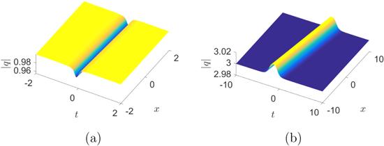
Figure 4. Dark and anti-dark soltion solutions with (a) λ1 = 2i, λ2 = −2.01i, a = 1, b = 12.99; (b) λ1 = i, λ2 = −1.01i, a = −3, b = 5.01. |
Case 8: Breather and rogue wave solutions
Let ${\lambda }_{1}=\pm {\lambda }_{2}^{* }$, we can gain the typical breather solution of equation (3 ), which is displayed in figure 5. Next, the rogue wave solution is derived from its breather solution through a limit process. Take one pair of negative complex-conjugate eigenvalues ${\lambda }_{1}=-{\lambda }_{2}^{* }$ and set $b=-2{\lambda }_{{\rm{R}}}^{2}+2{\lambda }_{{\rm{I}}}^{2}$, we can obtain the rogue wave solution by letting a → 2λI.
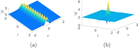
Figure 5. Breather and rogue wave solutions with (a) ${\lambda }_{1}={\lambda }_{2}^{* }=1+{\rm{i}},a=1,b=1$; (b) λ1 = −1 + i, λ2 = 1+i. |
Case 9: Double periodic solution
To describe the double periodic solution, we take Re(λ1) = Re(λ2) = 0, see figure 6. Interestingly, if we choose Im(λ2) to approach Im(λ1), the period of this solution will decrease. Set Im(λ2) → Im(λ1), the solution consisting of periodic waves and a breather is derived when a > b . Then the case a < b gives the shape of the solution as the anti-dark solution in figure 7.

Figure 6. Double periodic solution with λ1 = 1.1i, λ2 = i, a = 2, b = 1. |
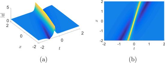
Figure 7. Mixed soliton solution with λ1 = 1.1i, λ2 = 0.8i, a = 1, b = 1.5. |
Case 10: Mixed kink and periodic solution
To derive the hybrid solution composing of a kink solution and a periodic solution, we choose the parameters as Re(λ1) = 0. We can obtain the interaction of periodic and kink solution which is shown in figure 8. This kind of solution can be regarded as a periodic solution with changed background height.
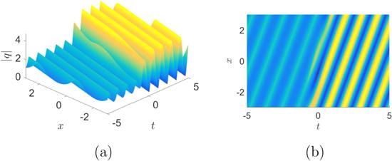
Figure 8. Mixed kink and periodic solution with λ1 = i, λ2 = 0.4 − i, a = 1.5, b = 0.5. |
3.2.2. Soliton solutions from nonzero seed solution by four-fold DT
Substituting eigenfunction (17 ) into (10 ) with N = 4, we can construct two-soliton solution from nonzero seed solution with the help of four-fold DT. Under these circumstances, [17] has obtained higher order rogue wave solutions by a certain limit. In our work, we provide some mixed soliton solutions in this subsection.
Case 11: Mixed rogue wave and periodic solution
For convenience, let b = 0, a = 1 and we take the limit of (17 ) at ${\lambda }_{1}=\tfrac{a}{2}+\tfrac{a}{2}{\rm{i}}$ and ${\lambda }_{2}=-\tfrac{a}{2}+\tfrac{a}{2}{\rm{i}}$, respectively. Then choose the appropriate parameters λ3 and λ4, the mixed rogue wave and periodic solution is derived in figure 9.
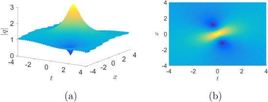
Figure 9. Mixed rogue wave and periodic solution with a = 1, b = 0, λ1 = 0.5 + 0.5i, λ2 = −0.5 + 0.5i, λ3 = 1.61i, λ4 = −1.6i. |
Case 12: Mixed W-shaped soliton and periodic solution
Let Re(λi) = 0 (i = 1, ⋯, 4), the mixed periodic solution is obtained through 4-fold DT. Next, we select the appropriate eigenvalues to construct new solutions of the nonlocal GI equation. In the case of Re(λ2) → −Re(λ1) and Re(λ3) → −Re(λ4), q[4] provides the mixed W(M)-shaped soliton and periodic solution. The soliton solution show special contours in that it is look like an English letter W(M). It is noteworthy that q[4] gives the M-shaped soliton while Im(λ1) < 0. Moreover it generates the W-shaped soliton while Im(λ1) > 0, which can see in figures 10 and 11.
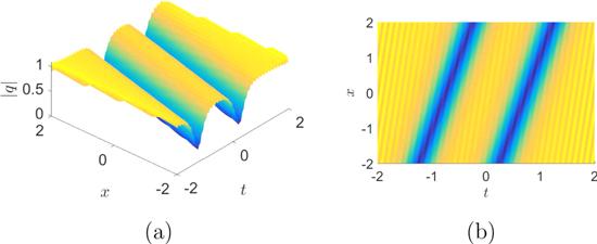
Figure 10. Mixed W-shaped soliton and periodic solution with λ1 = i, λ2 = −1.01i, λ3 = 2i, λ4 = −2.01i, a = 1, b = 2. |
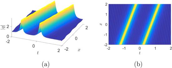
Figure 11. Mixed M-shaped soliton and periodic solution with λ1 = −i, λ2 = 1.01i, λ3 = −2i, λ4 = 2.01i, a = 1, b = 2. |
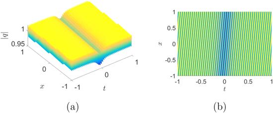
Case 13: Mixed dark soliton and periodic solution
Similar to case 12, when Re(λi) = 0 (i = 1, ⋯,4), the mixed dark soliton and periodic solution is derived from 4-fold DT by choosing appropriate parameters. Figure 12 displays the profiles of the special solution, which is like an unfolded book.
Figure 12. Mixed dark soliton and periodic solution with λ1 = −i, λ2 = 1.01i, λ3 = 2i, λ4 = −2.01i, a = 1, b = 12.99. |
Comparing the eigenfunctions of the local and nonlocal equations, the differences between the exact solutions of two equations in nonzero seed case are listed in table 1. We find the latter has fewer restrictive conditions, which has more parameter choices. It is necessary to find that the eigenfunctions in nonlocal equation are more general. What's more, the parameters a, b from nonzero seed solutions are complex constants in nonlocal GI equation. It is easy to find that the exact solutions of equation (3 ) possesses new characteristics in nonlocal case.
Table 1. Differences between the solutions of two equations in nonzero seed case. |
| Equation | GI equation | Nonlocal GI equation |
|---|---|---|
| Parameters a, b | Real | Complex |
| Discrepancies of solutions | Breather, rogue wave, dark soliton, periodic solutions | Breather, rogue wave, dark soliton, double periodic, kink, W/M-shape soliton solutions |
4. Conclusion
In this paper, the exact solutions in terms of the determinant have been represented based on 2n-fold DT. Through the distinct choices of parameters, we present several types of hybrid soliton solutions including bright-dark soliton, breather, rogue wave, periodic, W-shaped soliton and kink solutions. We devote to find the differences between local and nonlocal case. It is noteworthy that the solutions of the nonlocal GI equation are different from those of classic GI equation. We expect to find more types of explicit solutions which can then be presented in new features in the future.