


Nomenclature
$a$ radius of a superellipse
${B}_{o}$ magnetic field
$C$ concentration
${D}_{1}$ mass flux
${D}_{{\rm{m}}}$ mass diffusivity
$Du$ Dufour number
${D}_{2}$ heat flux
$n$ superellipse coefficient
${\rm{g}}$ gravity, $\left({\rm{m}}\,{{\rm{s}}}^{-2}\right)$
$p$ pressure, $\left({\rm{N}}\,{{\rm{m}}}^{-2}\right)$
$L$ cavity length
$\overline{Nu}$ mean Nusselt number
$\overline{Sh}$ mean Sherwood number
$u,\,v$ velocities, $\left({\rm{m}}\,{{\rm{s}}}^{-1}\right)$
$k$ thermal conductivity, $\left({\rm{W}}\,{{\rm{m}}}^{-1}\,{{\rm{K}}}^{-1}\right)$
$T$ temperature, $\left({\rm{K}}\right)$
$t$ time, $\left({\rm{s}}\right)$
${C}_{p}$ specific heat, $\left({{\rm{Jkg}}}^{-1}\,{{\rm{K}}}^{-1}\right)$
$X,\,Y$ dimensionless Cartesian coordinates
$U,\,V$ dimensionless velocities
$x,\,y$ Cartesian coordinates, ${\rm{m}}$
$\gamma $ magnetic incline angle
$\phi $ nanoparticle parameter
${\rm{\Phi }}$ dimensionless concentration
$\mu $ viscosity
$\beta $ thermal expansion coefficient $\left({{\rm{K}}}^{-1}\right)$
$\theta $ dimensionless temperature
$\tau $ dimensionless time
$\rho $ density, $\left({\rm{kg}}\,{{\rm{m}}}^{-3}\right)$
$\nu $ kinematic viscosity, $\left({{\rm{m}}}^{2}\,{{\rm{s}}}^{-1}\right)$
$\sigma $ electrical conductivity
$\psi $ stream function, $\left({{\rm{m}}}^{2}\,{{\rm{s}}}^{-1}\right)$
$\alpha $ thermal diffusivity, $\left({{\rm{m}}}^{2}\,{{\rm{s}}}^{-1}\right)$
$c$ low
$nf$ nanofluid
$f$ fluid
$h$ high
$np$ nanoparticles
1. Introduction
| • | The increase in the Hartmann number $Ha,$ nanoparticles parameter $\phi ,$ and radius of a superellipse $a$ is slowing down the nanofluid speed in an annulus. |
| • | The values of $\overline{Nu}$ and $\overline{Sh}$ are augmenting as nanoparticles parameter $\phi ,$ Rayleigh number $Ra,$ amplitude $A,$ and frequency $f$ are increasing. |
| • | Increasing $Sr$ with minimizing $Du$ is improving the strength of the concentration distributions in an annulus, and accordingly $\overline{Sh}$ is strongly decreasing. |
2. Mathematical analysis
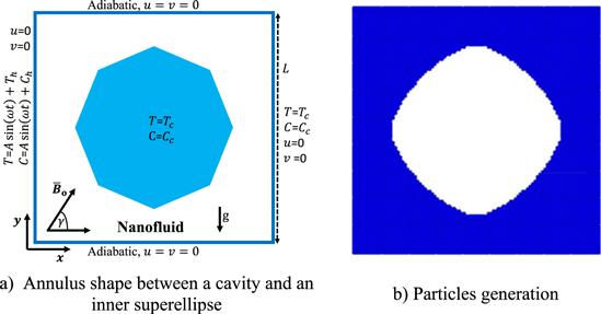
Figure 1. Geometry of the problem. |
| • | The Boussinesq approximation is utilized, in which density variations are ignored except via the gravity term. |
| • | The inclined magnetic field $\left(\overline{{B}_{0}}\right)$ used with an incline angle $\gamma $ along $x-y$ axis with ignoring the viscous dissipation and Joule heating impacts. |
| • | One phase model is employed for nanofluid modeling. |
| • | The fluid flow is laminar, incompressible, and transitional. |
2.1. Dimensionless boundary conditions
2.2. Nanofluid thermophysical properties
| $\beta \,\left(1/{\rm{K}}\right)$ | $\rho \,\left({\rm{kg}}\,{{\rm{m}}}^{-3}\right)$ | $k\,\left({\rm{W}}\,{{\rm{m}}}^{-1}\,{{\rm{K}}}^{-1}\right)$ | ${C}_{P}\left({\rm{J}}\,{\mathrm{kg}}^{-1}\,{{\rm{K}}}^{-1}\right)$ | $\sigma \,\left({\rm{S}}\,{{\rm{m}}}^{-1}\right)$ | |
|---|---|---|---|---|---|
| Copper | 1.67 $\times \,$10–5 | $8933$ | $401$ | $385$ | $5.96\,\times {10}^{7}$ |
| H2O | 21 $\times \,$10–5 | $997.1$ | $0.613$ | $4179$ | $0.05$ |
3. ISPH formulation
3.1. Solving steps
3.2. Validation of the ISPH method
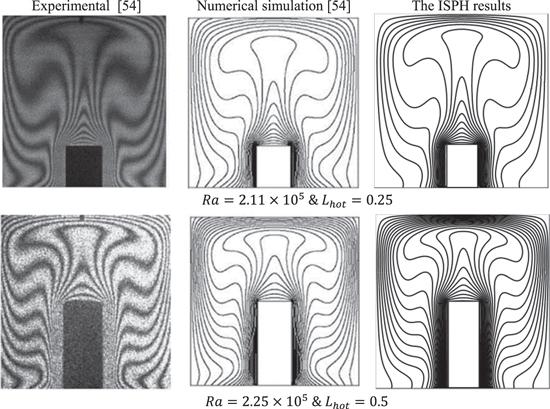
Figure 2. Isotherms of the numerical and experimental results of [54] and the ISPH results. |
4. Results and discussion
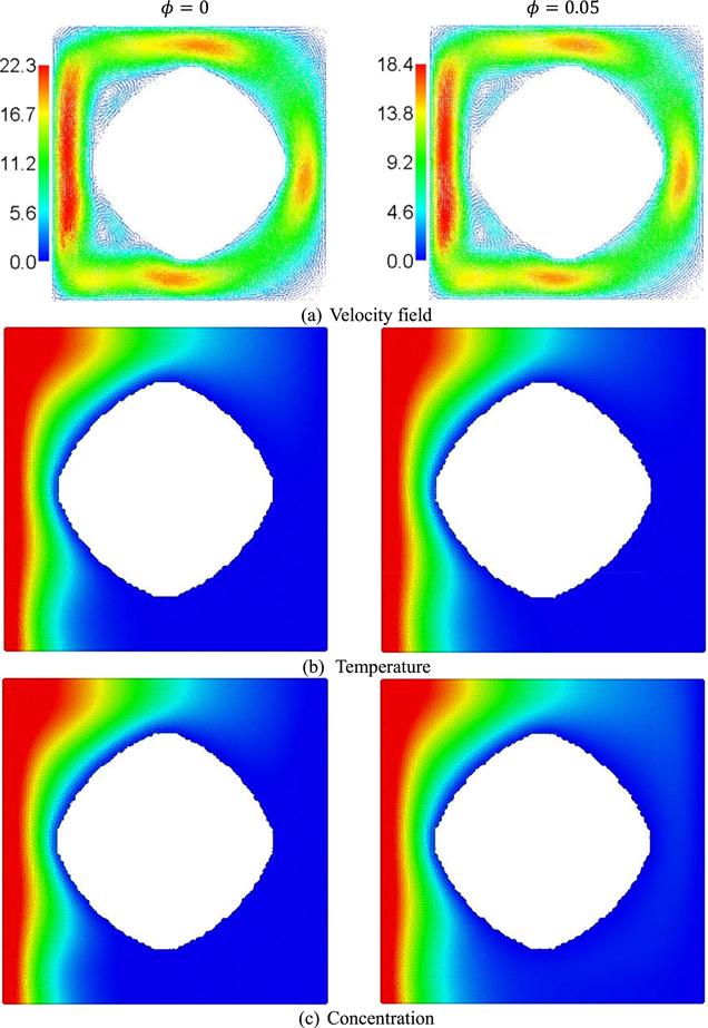
Figure 3. The influences of nanoparticle's parameter $\phi $ on nanofluid velocity, and deployments of temperature and concentration at $\gamma =45^\circ ,N=1,n=3/2,$ $a=0.35,Ra={10}^{4},$ $A=0.5,f=5,$ $Sr=1,Du=0.12,$ and $Ha=10.$ |
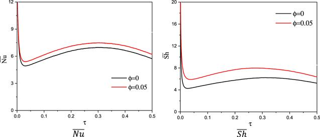
Figure 4. The values of $\overline{Nu}$ and $\overline{Sh}$ below the influences of the nanoparticle's parameter at $\gamma =45^\circ ,N=1,n=3/2,$ $a=0.35,Ra={10}^{4},$ $A=0.5,f=5,$ $Sr=1,Du=0.12,$ and $Ha=10.$ |

Figure 5. The influences of the Hartmann number on nanofluid velocity, and deployments of temperature and concentration at $\gamma =45^\circ ,N=1,$ $n=3/2,a=0.35,$ $Ra={10}^{4},$ $A=0.5,f=5,$ $Sr=1,Du=0.12,$ and $\phi =0.06.$ |
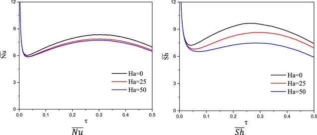
Figure 6. The values of $\overline{Nu}$ and $\overline{Sh}$ below the influences of the Hartmann number at $\gamma =45^\circ ,N=1,n=3/2,$ $a=0.35,Ra={10}^{4},$ $A=0.5,f=5,$ $Sr=1,Du=0.12,$ and $\phi =\mathrm{0.06.}$ |
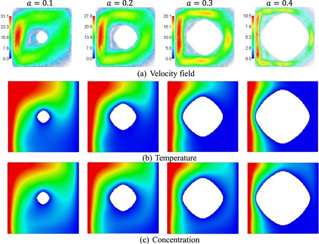
Figure 7. The influences of coefficient $a$ for a superellipse on nanofluid velocity, and deployments of temperature and concentration at $\gamma =45^\circ ,N=1,n=3/2,$ $Ha=10,Ra={10}^{4},$ $A=0.5,f=5,$ $Sr=1,Du=0.12,$ and $\phi =\mathrm{0.06.}$ |
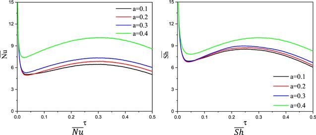
Figure 8. The values of $\overline{Nu}$ and $\overline{Sh}$ below the influences of the radius of a superellipse $a$ at $\gamma =45^\circ ,N=1,n=3/2,$ $Ha=10,Ra={10}^{4},$ $A=0.5,f=5,$ $Sr=1,Du=0.12,$ and $\phi =\mathrm{0.06.}$ |
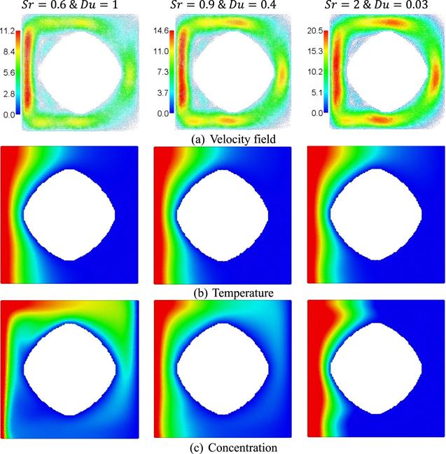
Figure 9. The influences of the Soret and Dufour parameters on nanofluid velocity, and deployments of temperature and concentration at $\gamma =45^\circ ,N=1,n=3/2,$ $a=0.35,Ha=10,$ $Ra={10}^{4},A=0.5,f=5,$ and $\phi =\mathrm{0.06.}$ |

Figure 10. The values of $\overline{Nu}$ and $\overline{Sh}$ below the influences of Soret and Dufour numbers at $\gamma =45^\circ ,N=1,$ $n=3/2,$ $a=0.35,Ha=10,$ $Ra={10}^{4},$ $A=0.5,f=5,$ and $\phi =\mathrm{0.06.}$ |

Figure 11. The influences of $Ra$ on nanofluid velocity, and deployments of temperature and concentration at $\gamma =45^\circ ,N=1,$ $n=3/2,a=0.35,$ $Ha=10,$ $A=0.5,f=5,$ $Sr=1,Du=0.12,$ and $\phi =\mathrm{0.06.}$ |

Figure 12. The values of $\overline{Nu}$ and $\overline{Sh}$ below the influences of the $Ra$ at $\gamma =45^\circ ,N=1,$ $n=3/2,a=0.35,$ $Ha=10,$ $A=0.5,f=5,$ $Sr=1,Du=0.12,$ and $\phi =\mathrm{0.06.}$ |

Figure 13. The influences of the amplitude and frequency of the temperature and concentration oscillation on the velocity field at $\gamma =45^\circ ,N=1,$ $n=3/2,a=0.35,$ $Ha=10,$ $Ra={10}^{4},$ $Sr=1,Du=0.12,$ and $\phi =\mathrm{0.06.}$ |

Figure 14. The influences of the amplitude and frequency of the temperature and concentration oscillation on the temperature at $\gamma =45^\circ ,N=1,n=3/2,a=0.35,Ha=10,$ $Ra={10}^{4},Sr=1,Du=0.12,$ and $\phi =0.06.$ |

Figure 15. The influences of the amplitude and frequency of the temperature and concentration oscillation on the concentration at $\gamma =45^\circ ,N=1,n=3/2,$ $a=0.35,Ha=10,$ $Ra={10}^{4},$ $Sr=1,Du=0.12,$ and $\phi =\mathrm{0.06.}$ |

Figure 16. 3D-plot of $\overline{Nu}$ and $\overline{Sh}$ below the influences of the amplitude and frequency of the temperature and concentration oscillation at $\gamma =45^\circ ,N=1,$ $n=3/2,a=0.35,$ $Ha=10,$ $Ra={10}^{4},$ $Sr=1,Du=0.12,$ and $\phi =\mathrm{0.06.}$ |