


1. Introduction
FPDEs are commonly used to describe problems in fluid mechanics, geographies, plasma physics, and thermal and mechanical systems. Increasing attention has been given by different scientists to find the exact solution for the fractional order reasoning. Many methods are being developed and are gradually maturing [3–9].
In this paper, the (3+1)-dimensional FTSKP equation is under investigation. This equation is used to analyze the complex dust acoustic wave structures [10, 11]. Diverse families of hyperbolic, trigonometric and plane wave solutions are constructed with different arguments. The new MEDA method [12–15] is adopted to derive the exact solutions. The (3+1)-dimensional FTSKP equation is read as follow [16, 17];
$\begin{eqnarray}\begin{array}{l}{{\rm{D}}}_{t}^{\alpha }{{\rm{D}}}_{x}^{\alpha }u+{a}_{1}{\left({{\rm{D}}}_{x}^{\alpha }u\right)}^{2}+{a}_{1}u{{\rm{D}}}_{x}^{2\alpha }u\\ +{a}_{2}{{\rm{D}}}_{x}^{4\alpha }u+{a}_{3}{{\rm{D}}}_{y}^{2\alpha }u+{a}_{3}{{\rm{D}}}_{z}^{2\alpha }u=0.\end{array}\end{eqnarray}$
In recent decades, exact solutions [18], analytical solutions [19] and numerical solutions [20] of many NPDEs have been successfully obtained. For example, the construction of bright-dark solitary waves and elliptic function solutions are observed in [21]. A fractional order model was used to find lump solutions in dusty plasma [22]. Dispersive shock wave solutions were also constructed in [23]. There are also many different methods for obtaining exact explicit solutions; the exp-function method [24, 25], the MEDA method [26], the extended auxiliary equation method [27] and modified method of simplest equation, the $(G^{\prime} /{G}^{2})$-expansion method [28], modified mapping method [29], extended homogeneous balance method [30] and extended Fan's sub-equation method [31], Lie algebraic discussion for affinity based information diffusion in social networks; analytical solution for an in-host viral infection model with time-inhomogeneous rates [32–34]; extended and modified direct algebraic method, extended mapping method, and Seadawy techniques [35–43].2. Wave propagation
To find the exact solutions of equation (1 ) we convert it into an ordinary differential equation by using the following transformation1 ) changes into the fractional order ordinary deferential equation as3 ) can be expressed as U(ξ) in the form of [15].3 ). Here we take4 ) is taken by homogeneous balancing principle from equation (3 ) by putting equal to highest derivative term and highest nonlinear term. It gives N = 1 and takes expression from the solutions of equation (4 ) as6 ) and its derivatives in equation (3 ) and equating the co-efficients of the same power of Q(ξ) equal to zero, we get the system of equations easily. We further solve this system of equations by using the mathematica or maple, and get the solutions set as follows:
$\begin{eqnarray}\begin{array}{l}u(x,y,z,t)=U(\xi ),\quad {\rm{where}}\\ \xi =\displaystyle \frac{p}{\alpha }{x}^{\alpha }+\displaystyle \frac{q}{\alpha }{y}^{\alpha }+\displaystyle \frac{r}{\alpha }{z}^{\alpha }-\displaystyle \frac{c}{\alpha }{t}^{\alpha }.\end{array}\end{eqnarray}$
Equation ( $\begin{eqnarray}\begin{array}{l}{{pcU}}^{{\prime\prime} }(\xi )+{\alpha }_{1}{\left({{pU}}^{{\prime} }(\xi )\right)}^{2}+{\alpha }_{1}{{pUU}}^{{\prime\prime} }(\xi )\\ +{\alpha }_{2}{p}^{4}{U}^{{\prime} \prime\prime\prime }(\xi )+{\alpha }_{3}{q}^{2}{U}^{{\prime\prime} }(\xi )+{\alpha }_{3}{r}^{2}{U}^{{\prime\prime} }(\xi )=0.\end{array}\end{eqnarray}$
Suppose the solutions of equation ( $\begin{eqnarray}U(\xi )=\sum _{i=0}^{N}{b}_{i}{Q}^{i}(\xi ),\quad {b}_{i}\ne 0,\end{eqnarray}$
where bi(0 ≤ i ≤ N) are constants and Q(ξ) is satisfy the equation ( $\begin{eqnarray}\begin{array}{l}{Q}^{{\prime} }(\xi )=\mathrm{ln}(B)(\mu +\lambda Q(\xi )+{{rQ}}^{2}(\xi ))\\ B\ne 0,1\end{array}\end{eqnarray}$
The value of N for equation ( $\begin{eqnarray}u(\xi )={b}_{0}+{b}_{1}Q(\xi ).\end{eqnarray}$
Substituting equation (Case 1: where free parameters are r and μ while along with b0 = 0, ${b}_{1}=-\tfrac{6\sqrt{5}\sqrt{{\alpha }_{2}}{pr}\mathrm{ln}(B)\sqrt{{cp}+{\alpha }_{3}{q}^{2}+{\alpha }_{3}{s}^{2}}}{{\alpha }_{1}+{\alpha }_{1}p}$,$\lambda =\tfrac{\sqrt{{\alpha }_{3}{q}^{2}+{\alpha }_{3}{s}^{2}}}{\sqrt{5}\sqrt{{\alpha }_{2}}{p}^{2}\mathrm{ln}(B)}$
Type 1: For λ2 − μr < 0 and r ≠ 0, the mixed trigonometric solutions are found as
$\begin{eqnarray*}\begin{array}{l}{u}_{1}(\xi )=-\displaystyle \frac{6\sqrt{5}\sqrt{{\alpha }_{2}}{pr}\mathrm{ln}(B)\sqrt{{cp}+{\alpha }_{3}{q}^{2}+{\alpha }_{3}{s}^{2}}}{{\alpha }_{1}+{\alpha }_{1}p}\\ \times \left(-\displaystyle \frac{\sqrt{{\alpha }_{3}{q}^{2}+{\alpha }_{3}{s}^{2}}}{2\sqrt{5}\sqrt{{\alpha }_{2}}{{rp}}^{2}\mathrm{ln}(B)}+\displaystyle \frac{\sqrt{-\left(\tfrac{{\alpha }_{3}({q}^{2}+{s}^{2})}{5{\alpha }_{2}{p}^{4}{\mathrm{ln}}^{2}(B)}-4\mu r\right)}}{2r}\right.\\ \left.{\tan }_{B}\left(\displaystyle \frac{\sqrt{-(\tfrac{{\alpha }_{3}({q}^{2}+{s}^{2})}{5{\alpha }_{2}{p}^{4}{\mathrm{ln}}^{2}(B)}-4\mu r)}}{2}\xi \right)\right).\end{array}\end{eqnarray*}$
The plot and its corresponding contour plot of the solution u1(x, t) are depicted in figure 1, for the different choices of parameters c = 100, p = 100.101, μ = 0.1, s = 0.0005, α1 =20, α2 = 0.9, α3 = 1, r = 0.0002, q = 0.1, and B = 5. $\begin{eqnarray*}\begin{array}{l}{u}_{2}(\xi )=-\displaystyle \frac{6\sqrt{5}\sqrt{{\alpha }_{2}}{pr}\mathrm{ln}(B)\sqrt{{cp}+{\alpha }_{3}{q}^{2}+{\alpha }_{3}{s}^{2}}}{{\alpha }_{1}+{\alpha }_{1}p}\\ \times \left(-\displaystyle \frac{\sqrt{{\alpha }_{3}{q}^{2}+{\alpha }_{3}{s}^{2}}}{2\sqrt{5}\sqrt{{\alpha }_{2}}{{rp}}^{2}\mathrm{ln}(B)}-\displaystyle \frac{\sqrt{-\left(\tfrac{{\alpha }_{3}({q}^{2}+{s}^{2})}{5{\alpha }_{2}{p}^{4}{\mathrm{ln}}^{2}(B)}-4\mu r\right)}}{2r}\right.\\ \left.{\cot }_{B}\left(\displaystyle \frac{\sqrt{-\left(\tfrac{{\alpha }_{3}({q}^{2}+{s}^{2})}{5{\alpha }_{2}{p}^{4}{\mathrm{ln}}^{2}(B)}-4\mu r\right)}}{2}\xi \right)\right).\end{array}\end{eqnarray*}$
The plot and its corresponding contour plot of the solution u1(x, t) are depicted in figure 2, for the values of parameters c = 120, p = 1, μ = 0.1, s = 0.0005, α1 = 20, α2 = 0.9, α3 = 1, q = 0.0002, q = 0.1, and B = 5. $\begin{eqnarray*}\begin{array}{l}{u}_{3}(\xi )=-\displaystyle \frac{6\sqrt{5}\sqrt{{\alpha }_{2}}{pr}\mathrm{ln}(B)\sqrt{{cp}+{\alpha }_{3}{q}^{2}+{\alpha }_{3}{s}^{2}}}{{\alpha }_{1}+{\alpha }_{1}p}\\ \times \left(-\displaystyle \frac{\sqrt{{\alpha }_{3}{q}^{2}+{\alpha }_{3}{s}^{2}}}{2\sqrt{5}\sqrt{{\alpha }_{2}}{{rp}}^{2}\mathrm{ln}(B)}+\displaystyle \frac{\sqrt{-\left(\tfrac{{\alpha }_{3}({q}^{2}+{s}^{2})}{5{\alpha }_{2}{p}^{4}{\mathrm{ln}}^{2}(B)}-4\mu r\right)}}{2r}\right.\\ \left({\tan }_{B}\left(\sqrt{-\left(\displaystyle \frac{{\alpha }_{3}({q}^{2}+{s}^{2})}{5{\alpha }_{2}{p}^{4}{\mathrm{ln}}^{2}(B)}-4\mu r\right)}\xi \right)\right.\\ \left.\left.\pm \sqrt{({pq})}{\sec }_{B}\left(\sqrt{-\left(\displaystyle \frac{{\alpha }_{3}({q}^{2}+{s}^{2})}{5{\alpha }_{2}{p}^{4}{\mathrm{ln}}^{2}(B)}-4\mu r\right)}\xi \right)\right)\right).\end{array}\end{eqnarray*}$
The plot and its corresponding contour plot of the solutions u3(x, t) are depicted in figure 3, for the values of parameters c = 20, p = 20, μ = 2.1, s = 10.5, α1 = 20, α2 = 0.9, α3 = 1, q = 2.2, q = 1.1, and B = 2. $\begin{eqnarray*}\begin{array}{l}{u}_{4}(\xi )=-\displaystyle \frac{6\sqrt{5}\sqrt{{\alpha }_{2}}{pr}\mathrm{ln}(B)\sqrt{{cp}+{\alpha }_{3}{q}^{2}+{\alpha }_{3}{s}^{2}}}{{\alpha }_{1}+{\alpha }_{1}p}\\ \times \left(-\displaystyle \frac{\sqrt{{\alpha }_{3}{q}^{2}+{\alpha }_{3}{s}^{2}}}{2\sqrt{5}\sqrt{{\alpha }_{2}}{{rp}}^{2}\mathrm{ln}(B)}-\displaystyle \frac{\sqrt{-\left(\tfrac{{\alpha }_{3}({q}^{2}+{s}^{2})}{5{\alpha }_{2}{p}^{4}{\mathrm{ln}}^{2}(B)}-4\mu r\right)}}{2r}\right.\\ \left({\cot }_{B}\left(\sqrt{-\left(\displaystyle \frac{{\alpha }_{3}({q}^{2}+{s}^{2})}{5{\alpha }_{2}{p}^{4}{\mathrm{ln}}^{2}(B)}-4\mu r\right)}\xi \right)\right.\\ \left.\left.\pm \sqrt{({pq})}{\csc }_{B}\left(\sqrt{-\left(\displaystyle \frac{{\alpha }_{3}({q}^{2}+{s}^{2})}{5{\alpha }_{2}{p}^{4}{\mathrm{ln}}^{2}(B)}-4\mu r\right)}\xi \right)\right)\right).\end{array}\end{eqnarray*}$
The plot and its corresponding contour plot of the solutions u4(x, t) are depicted in figure 4, for the values of parameters c = 10, p = 20, μ = 21, s = 15, α1 = 30, α2 = 1.9, α3 = 10, q = 22.2, q = 1.1, and B = 5. $\begin{eqnarray*}\begin{array}{l}{u}_{5}(\xi )=-\displaystyle \frac{6\sqrt{5}\sqrt{{\alpha }_{2}}{pr}\mathrm{ln}(B)\sqrt{{cp}+{\alpha }_{3}{q}^{2}+{\alpha }_{3}{s}^{2}}}{{\alpha }_{1}+{\alpha }_{1}p}\\ \times \left(-\displaystyle \frac{\sqrt{{\alpha }_{3}{q}^{2}+{\alpha }_{3}{s}^{2}}}{2\sqrt{5}\sqrt{{\alpha }_{2}}{{rp}}^{2}\mathrm{ln}(B)}+\displaystyle \frac{\sqrt{-\left(\tfrac{{\alpha }_{3}({q}^{2}+{s}^{2})}{5{\alpha }_{2}{p}^{4}{\mathrm{ln}}^{2}(B)}-4\mu r\right)}}{2r}\right.\\ \left({\tan }_{B}\left(\displaystyle \frac{\sqrt{-\left(\tfrac{{\alpha }_{3}({q}^{2}+{s}^{2})}{5{\alpha }_{2}{p}^{4}{\mathrm{ln}}^{2}(B)}-4\mu r\right)}}{4}\xi \right)\right.\\ \left.\left.-\sqrt{({pq})}{\cot }_{B}\left(\displaystyle \frac{\sqrt{-\left(\tfrac{{\alpha }_{3}({q}^{2}+{s}^{2})}{5{\alpha }_{2}{p}^{4}{\mathrm{ln}}^{2}(B)}-4\mu r\right)}}{4}\xi \right)\right)\right).\end{array}\end{eqnarray*}$
The plot and its corresponding contour plot of the solutions u5(x, t) are depicted in figure 5, for the values of parameters c = 10, p = 20, μ = 21, s = 15, α1 = 30, α2 = 1.9, α3 = 10, q = 22.2, q = 1.1, and B = 5.
Figure 1. Graphical representation and corresponding contour of u1(x, t) for different values of parameters. |

Figure 2. Graphical representation and corresponding contour of u2(x, t) for different values of parameters. |
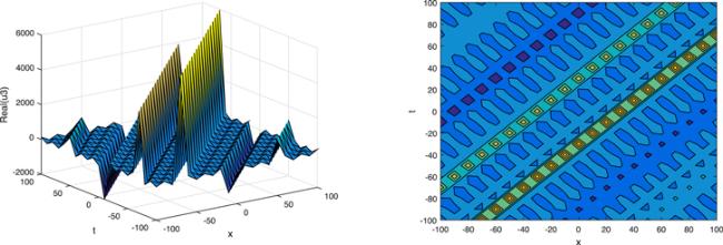
Figure 3. Graphical representation and corresponding contour of u3(x, t) for different values of parameters. |
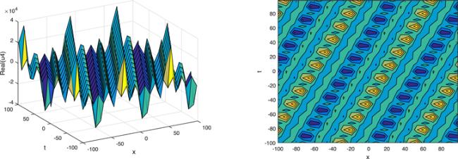
Figure 4. Graphical representation and corresponding contour of u4(x, t) for different values of parameters. |

Figure 5. Graphical representation and corresponding contour of u5(x, t) for different values of parameters. |
Type 2: For λ2 − μr > 0 and r ≠ 0, different types of solutions are obtained.
The dark solutions are obtained as
$\begin{eqnarray*}\begin{array}{l}{u}_{6}(\xi )=-\displaystyle \frac{6\sqrt{5}\sqrt{{\alpha }_{2}}{pr}\mathrm{ln}(B)\sqrt{{cp}+{\alpha }_{3}{q}^{2}+{\alpha }_{3}{s}^{2}}}{{\alpha }_{1}+{\alpha }_{1}p}\\ \times \left(-\displaystyle \frac{\sqrt{{\alpha }_{3}{q}^{2}+{\alpha }_{3}{s}^{2}}}{2\sqrt{5}\sqrt{{\alpha }_{2}}{{rp}}^{2}\mathrm{ln}(B)}+\displaystyle \frac{\sqrt{-\left(\tfrac{{\alpha }_{3}({q}^{2}+{s}^{2})}{5{\alpha }_{2}{p}^{4}{\mathrm{ln}}^{2}(B)}-4\mu r\right)}}{2r}\right.\\ \left.{\tanh }_{B}\left(\displaystyle \frac{\sqrt{-(\tfrac{{\alpha }_{3}({q}^{2}+{s}^{2})}{5{\alpha }_{2}{p}^{4}{\mathrm{ln}}^{2}(B)}-4\mu r)}}{2}\xi \right)\right).\end{array}\end{eqnarray*}$
The plot and its corresponding contour plot of the solutions u6(x, t) are depicted in figure 6, for the values of parameters c = 10, p = 10.101, μ = 0.1, s = 11.5, α1 = 20, α2 = 0.9, α3 = 1, q = 0.0002, q = 0.1, and B = 5.
Figure 6. Graphical representation and corresponding contour of u6(x, t) for different values of parameters. |
The singular solution is obtained as
$\begin{eqnarray*}\begin{array}{l}{u}_{7}(\xi )=-\displaystyle \frac{6\sqrt{5}\sqrt{{\alpha }_{2}}{pr}\mathrm{ln}(B)\sqrt{{cp}+{\alpha }_{3}{q}^{2}+{\alpha }_{3}{s}^{2}}}{{\alpha }_{1}+{\alpha }_{1}p}\\ \times \left(-\displaystyle \frac{\sqrt{{\alpha }_{3}{q}^{2}+{\alpha }_{3}{s}^{2}}}{2\sqrt{5}\sqrt{{\alpha }_{2}}{{rp}}^{2}\mathrm{ln}(B)}-\displaystyle \frac{\sqrt{-\left(\tfrac{{\alpha }_{3}({q}^{2}+{s}^{2})}{5{\alpha }_{2}{p}^{4}{\mathrm{ln}}^{2}(B)}-4\mu r\right)}}{2r}\right.\\ \left.{\coth }_{B}\left(\displaystyle \frac{\sqrt{-\left(\tfrac{{\alpha }_{3}({q}^{2}+{s}^{2})}{5{\alpha }_{2}{p}^{4}{\mathrm{ln}}^{2}(B)}-4\mu r\right)}}{2}\xi \right)\right).\end{array}\end{eqnarray*}$
The complex dark bright solution is obtained as $\begin{eqnarray*}\begin{array}{l}{u}_{8}(\xi )=-\displaystyle \frac{6\sqrt{5}\sqrt{{\alpha }_{2}}{pr}\mathrm{ln}(B)\sqrt{{cp}+{\alpha }_{3}{q}^{2}+{\alpha }_{3}{s}^{2}}}{{\alpha }_{1}+{\alpha }_{1}p}\\ \times \left(-\displaystyle \frac{\sqrt{{\alpha }_{3}{q}^{2}+{\alpha }_{3}{s}^{2}}}{2\sqrt{5}\sqrt{{\alpha }_{2}}{{rp}}^{2}\mathrm{ln}(B)}-\displaystyle \frac{\sqrt{-\left(\tfrac{{\alpha }_{3}({q}^{2}+{s}^{2})}{5{\alpha }_{2}{p}^{4}{\mathrm{ln}}^{2}(B)}-4\mu r\right)}}{2r}\right.\\ \left({\tanh }_{B}\left(\sqrt{-\left(\displaystyle \frac{{\alpha }_{3}({q}^{2}+{s}^{2})}{5{\alpha }_{2}{p}^{4}{\mathrm{ln}}^{2}(B)}-4\mu r\right)}\xi \right)\right.\\ \left.\left.\pm {\rm{i}}\sqrt{({pq})}{{\rm{{\rm{sech}} }}}_{B}\left(\sqrt{-\left(\displaystyle \frac{{\alpha }_{3}({q}^{2}+{s}^{2})}{5{\alpha }_{2}{p}^{4}{\mathrm{ln}}^{2}(B)}-4\mu r\right)}\xi \right)\right)\right).\end{array}\end{eqnarray*}$
The plot and its corresponding contour plot of the solutions u6(x, t) are depicted in figure 7, for the values of parameters c = 100, p = 100, μ = 21, s = 10.5, α1 = 200, α2 = 10.9, α3 = 1, q = 20.2, q = 11, and B = 20.
Figure 7. Graphical representation and corresponding contour of u8(x, t) for different values of parameters. |
The mixed singular solution is obtained as
$\begin{eqnarray*}\begin{array}{l}{u}_{9}(\xi )=-\displaystyle \frac{6\sqrt{5}\sqrt{{\alpha }_{2}}{pr}\mathrm{ln}(B)\sqrt{{cp}+{\alpha }_{3}{q}^{2}+{\alpha }_{3}{s}^{2}}}{{\alpha }_{1}+{\alpha }_{1}p}\\ \times \left(-\displaystyle \frac{\sqrt{{\alpha }_{3}{q}^{2}+{\alpha }_{3}{s}^{2}}}{2\sqrt{5}\sqrt{{\alpha }_{2}}{{rp}}^{2}\mathrm{ln}(B)}-\displaystyle \frac{\sqrt{-\left(\tfrac{{\alpha }_{3}({q}^{2}+{s}^{2})}{5{\alpha }_{2}{p}^{4}{\mathrm{ln}}^{2}(B)}-4\mu r\right)}}{2r}\right.\\ \left({\coth }_{B}\left(\sqrt{-\left(\displaystyle \frac{{\alpha }_{3}({q}^{2}+{s}^{2})}{5{\alpha }_{2}{p}^{4}{\mathrm{ln}}^{2}(B)}-4\mu r\right)}\xi \right)\right.\\ \left.\left.\pm \sqrt{({pq})}{{\rm{csch}}}_{B}\left(\sqrt{-\left(\displaystyle \frac{{\alpha }_{3}({q}^{2}+{s}^{2})}{5{\alpha }_{2}{p}^{4}{\mathrm{ln}}^{2}(B)}-4\mu r\right)}\xi \right)\right)\right).\end{array}\end{eqnarray*}$
The dark solution is obtained as $\begin{eqnarray*}\begin{array}{l}{u}_{10}(\xi )=-\displaystyle \frac{6\sqrt{5}\sqrt{{\alpha }_{2}}{pr}\mathrm{ln}(B)\sqrt{{cp}+{\alpha }_{3}{q}^{2}+{\alpha }_{3}{s}^{2}}}{{\alpha }_{1}+{\alpha }_{1}p}\\ \times \left(-\displaystyle \frac{\sqrt{{\alpha }_{3}{q}^{2}+{\alpha }_{3}{s}^{2}}}{2\sqrt{5}\sqrt{{\alpha }_{2}}{{rp}}^{2}\mathrm{ln}(B)}+\displaystyle \frac{\sqrt{-\left(\tfrac{{\alpha }_{3}({q}^{2}+{s}^{2})}{5{\alpha }_{2}{p}^{4}{\mathrm{ln}}^{2}(B)}-4\mu r\right)}}{4r}\right.\\ \left({\tanh }_{B}\left(\displaystyle \frac{\sqrt{-\left(\tfrac{{\alpha }_{3}({q}^{2}+{s}^{2})}{5{\alpha }_{2}{p}^{4}{\mathrm{ln}}^{2}(B)}-4\mu r\right)}}{4}\xi \right)\right.\\ \left.\left.+{\coth }_{B}\left(\displaystyle \frac{\sqrt{-\left(\tfrac{{\alpha }_{3}({q}^{2}+{s}^{2})}{5{\alpha }_{2}{p}^{4}{\mathrm{ln}}^{2}(B)}-4\mu r\right)}}{4}\xi \right)\right)\right).\end{array}\end{eqnarray*}$
Type 3: For μr > 0 and λ = 0, we obtained trigonometric solutions as
$\begin{eqnarray*}\begin{array}{rcl}{u}_{11}(\xi ) & = & -\displaystyle \frac{6\sqrt{5}\sqrt{{\alpha }_{2}}{pr}\mathrm{ln}(B)\sqrt{{cp}+{\alpha }_{3}{q}^{2}+{\alpha }_{3}{s}^{2}}}{{\alpha }_{1}+{\alpha }_{1}p}\\ & & \times \left(\sqrt{\displaystyle \frac{\mu }{r}}{\tan }_{B}(\sqrt{\mu r}\xi )\right).\end{array}\end{eqnarray*}$
The plot and its corresponding contour plot of the solutions u11(x, t) are depicted in figure 8, for the values of parameters c = 80, p = 1.01, μ = 0.1, s = 0.05, α1 = 10, α2 = 0.9, α3 = 1, q = 0.002, q = 0.1, and B = 3. $\begin{eqnarray*}\begin{array}{rcl}{u}_{12}(\xi ) & = & \displaystyle \frac{6\sqrt{5}\sqrt{{\alpha }_{2}}{pr}\mathrm{ln}(B)\sqrt{{cp}+{\alpha }_{3}{q}^{2}+{\alpha }_{3}{s}^{2}}}{{\alpha }_{1}+{\alpha }_{1}p}\\ & & \times \left(\sqrt{\displaystyle \frac{\mu }{r}}{\cot }_{B}(\sqrt{\mu r}\xi )\right).\end{array}\end{eqnarray*}$
The plot and its corresponding contour plot of the solutions u12(x, t) are depicted in figure 9, for the values of parameters c = 80, p = 0.01, μ = 0.1, s = 0.05, α1 = 10, α2 = 0.9, α3 = 1, q = 0.002, q = 0.1, and B = 3.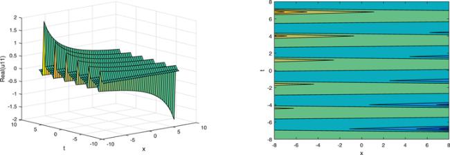
Figure 8. Graphical representation and corresponding contour of u11(x, t) for different values of parameters. |
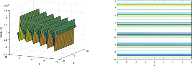
Figure 9. Graphical representation and corresponding contour of u12(x, t) for different values of parameters. |
The mixed trigonometric solutions are obtained as
$\begin{eqnarray*}\begin{array}{rcl}{u}_{13}(\xi ) & = & -\displaystyle \frac{6\sqrt{5}\sqrt{{\alpha }_{2}}{pr}\mathrm{ln}(B)\sqrt{{cp}+{\alpha }_{3}{q}^{2}+{\alpha }_{3}{s}^{2}}}{{\alpha }_{1}+{\alpha }_{1}p}\\ & & \times \sqrt{\displaystyle \frac{\mu }{r}}\left({\tan }_{B}(2\sqrt{\mu r}\xi )\pm \sqrt{{pq}}{\sec }_{B}(2\sqrt{\mu r}\xi )\right).\end{array}\end{eqnarray*}$
The plot and its corresponding contour plot of the solutions u13(x, t) are depicted in figure 10, for the values of parameters c = 100, p = 100, μ = 1.1, s = 1.05, α1 = 10, α2 = 0.9, α3 = 1, q = 0.02, q = 0.1, and B = 3. $\begin{eqnarray*}\begin{array}{rcl}{u}_{14}(\xi ) & = & \displaystyle \frac{6\sqrt{5}\sqrt{{\alpha }_{2}}{pr}\mathrm{ln}(B)\sqrt{{cp}+{\alpha }_{3}{q}^{2}+{\alpha }_{3}{s}^{2}}}{{\alpha }_{1}+{\alpha }_{1}p}\\ & & \times \sqrt{\displaystyle \frac{\mu }{r}}\left({\cot }_{B}\left(2\sqrt{\mu r}\xi \right)\pm \sqrt{{pq}}{\csc }_{B}\left(2\sqrt{\mu r}\xi \right)\right),\end{array}\end{eqnarray*}$
$\begin{eqnarray*}\begin{array}{rcl}{u}_{15}(\xi ) & = & -\displaystyle \frac{6\sqrt{5}\sqrt{{\alpha }_{2}}{pr}\mathrm{ln}(B)\sqrt{{cp}+{\alpha }_{3}{q}^{2}+{\alpha }_{3}{s}^{2}}}{{\alpha }_{1}+{\alpha }_{1}p}\\ & & \times \displaystyle \frac{1}{2}\sqrt{\displaystyle \frac{\mu }{r}}\left({\tan }_{B}(\displaystyle \frac{\sqrt{\mu r}}{2}\xi )-\sqrt{{pq}}{\cot }_{B}(\displaystyle \frac{\sqrt{\mu r}}{2}\xi )\right),\end{array}\end{eqnarray*}$
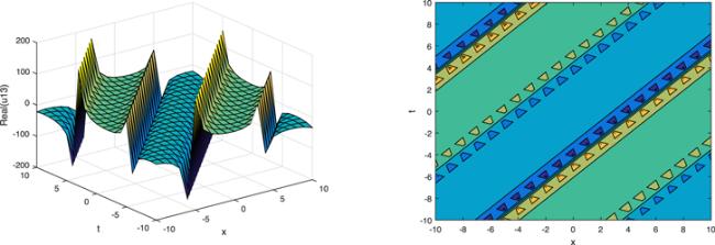
Figure 10. Graphical representation and corresponding contour of u13(x, t) for different values of parameters. |
Type 4: For μr < 0 and λ = 0, we obtained dark solutions as
$\begin{eqnarray*}\begin{array}{rcl}{u}_{16}(\xi ) & = & \displaystyle \frac{6\sqrt{5}\sqrt{{\alpha }_{2}}{pr}\mathrm{ln}(B)\sqrt{{cp}+{\alpha }_{3}{q}^{2}+{\alpha }_{3}{s}^{2}}}{{\alpha }_{1}+{\alpha }_{1}p}\\ & & \times \left(\sqrt{-\displaystyle \frac{\mu }{r}}{\tanh }_{B}(\sqrt{-\mu r}\xi )\right).\end{array}\end{eqnarray*}$
The plot and its corresponding contour plot of the solutions u16(x, t) are depicted in figure 11, for the values of parameters c = 80, p = 1.01, μ = 0.1, s = 0.05, α1 = 10, α2 = 0.9, α3 = 1, q = 0.02, q = 0.1, and B = 3. We get the singular solution as $\begin{eqnarray*}\begin{array}{rcl}{u}_{17}(\xi ) & = & \displaystyle \frac{6\sqrt{5}\sqrt{{\alpha }_{2}}{pr}\mathrm{ln}(B)\sqrt{{cp}+{\alpha }_{3}{q}^{2}+{\alpha }_{3}{s}^{2}}}{{\alpha }_{1}+{\alpha }_{1}p}\\ & & \times \left(\sqrt{-\displaystyle \frac{\mu }{r}}{\coth }_{B}(\sqrt{-\mu r}\xi )\right).\end{array}\end{eqnarray*}$
The plot and its corresponding contour plot of the solutions u17(x, t) are depicted in figure 12, for the values of parameters c = 80, p = 0.01, μ = 0.1, s = 0.05, α1 = 10, α2 = 0.9, α3 = 1, q = 0.002, q = 0.1, and B = 3.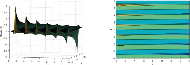
Figure 11. Graphical representation and corresponding contour of u16(x, t) for different values of parameters. |
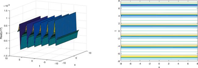
Figure 12. Graphical representation and corresponding contour of u17(x, t) for different values of parameters. |
The different type of complex combo solutions are obtained as
$\begin{eqnarray*}\begin{array}{l}{u}_{18}(\xi )=\displaystyle \frac{6\sqrt{5}\sqrt{{\alpha }_{2}}{pr}\mathrm{ln}(B)\sqrt{{cp}+{\alpha }_{3}{q}^{2}+{\alpha }_{3}{s}^{2}}}{{\alpha }_{1}+{\alpha }_{1}p}\\ \times \sqrt{-\displaystyle \frac{\mu }{r}}\left({\tanh }_{B}(2\sqrt{-\mu r}\xi )\pm {\rm{i}}\sqrt{{pq}}{{\rm{{\rm{sech}} }}}_{B}(2\sqrt{-\mu r}\xi )\right).\end{array}\end{eqnarray*}$
The plot and its corresponding contour plot of the solutions u18(x, t) are depicted in figure 13, for the values of parameters c = 100, p = 100, μ = 1.1, s = 1.05, α1 = 10, α2 = 0.9, α3 = 1, q = 0.02, q = 0.1, and B = 3. $\begin{eqnarray*}\begin{array}{l}{u}_{19}(\xi )=\displaystyle \frac{6\sqrt{5}\sqrt{{\alpha }_{2}}{pr}\mathrm{ln}(B)\sqrt{{cp}+{\alpha }_{3}{q}^{2}+{\alpha }_{3}{s}^{2}}}{{\alpha }_{1}+{\alpha }_{1}p}\\ \times \sqrt{-\displaystyle \frac{\mu }{r}}\left({\coth }_{B}(2\sqrt{-\mu r}\xi )\pm \sqrt{{pq}}{{csch}}_{B}(2\sqrt{-\mu r}\xi )\right),\end{array}\end{eqnarray*}$
$\begin{eqnarray*}\begin{array}{l}{u}_{20}(\xi )=-\displaystyle \frac{6\sqrt{5}\sqrt{{\alpha }_{2}}{pr}\mathrm{ln}(B)\sqrt{{cp}+{\alpha }_{3}{q}^{2}+{\alpha }_{3}{s}^{2}}}{{\alpha }_{1}+{\alpha }_{1}p}\\ \times \displaystyle \frac{1}{2}\sqrt{\displaystyle \frac{-\mu }{r}}\left({\tanh }_{B}(\displaystyle \frac{\sqrt{-\mu r}}{2}\xi )-{\coth }_{B}(\displaystyle \frac{\sqrt{-\mu r}}{2}\xi )\right).\end{array}\end{eqnarray*}$
The plot and its corresponding contour plot of the solutions u20(x, t) are depicted in figure 14, for the values of parameters c = 100, p = 100, μ = 1.1, s = 1.05, α1 = 10, α2 = 0.9, α3 = 1, q = 0.02, q = 0.1, and B = 3.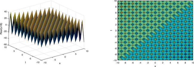
Figure 13. Graphical representation and corresponding contour of u18(x, t) for different values of parameters. |
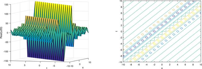
Figure 14. Graphical representation and corresponding contour of u20(x, t) for different values of parameters. |
Type 5: For λ = 0 and μ = r, the periodic and mixed periodic solutions are obtained as
$\begin{eqnarray*}\begin{array}{rcl}{u}_{21}(\xi ) & = & -\displaystyle \frac{6\sqrt{5}\sqrt{{\alpha }_{2}}{pr}\mathrm{ln}(B)\sqrt{{cp}+{\alpha }_{3}{q}^{2}+{\alpha }_{3}{s}^{2}}}{{\alpha }_{1}+{\alpha }_{1}p}\\ & & \times \left({\tan }_{B}(\mu \xi )\right),\end{array}\end{eqnarray*}$
$\begin{eqnarray*}\begin{array}{rcl}{u}_{22}(\xi ) & = & -\displaystyle \frac{6\sqrt{5}\sqrt{{\alpha }_{2}}{pr}\mathrm{ln}(B)\sqrt{{cp}+{\alpha }_{3}{q}^{2}+{\alpha }_{3}{s}^{2}}}{{\alpha }_{1}+{\alpha }_{1}p}\\ & & \times \left(-{\cot }_{B}(\mu \xi )\right),\end{array}\end{eqnarray*}$
$\begin{eqnarray*}\begin{array}{rcl}{u}_{23}(\xi ) & = & -\displaystyle \frac{6\sqrt{5}\sqrt{{\alpha }_{2}}{pr}\mathrm{ln}(B)\sqrt{{cp}+{\alpha }_{3}{q}^{2}+{\alpha }_{3}{s}^{2}}}{{\alpha }_{1}+{\alpha }_{1}p}\\ & & \times \left({\tan }_{B}(2\mu \xi )\pm \sqrt{{pq}}{\sec }_{B}(2\mu \xi )\right),\end{array}\end{eqnarray*}$
$\begin{eqnarray*}\begin{array}{rcl}{u}_{24}(\xi ) & = & \displaystyle \frac{6\sqrt{5}\sqrt{{\alpha }_{2}}{pr}\mathrm{ln}(B)\sqrt{{cp}+{\alpha }_{3}{q}^{2}+{\alpha }_{3}{s}^{2}}}{{\alpha }_{1}+{\alpha }_{1}p}\\ & & \times \left({\cot }_{B}(2\mu \xi )\pm \sqrt{{pq}}{{\csc }}_{B}(2\mu \xi )\right),\end{array}\end{eqnarray*}$
$\begin{eqnarray*}\begin{array}{rcl}{u}_{25}(\xi ) & = & -\displaystyle \frac{6\sqrt{5}\sqrt{{\alpha }_{2}}{pr}\mathrm{ln}(B)\sqrt{{cp}+{\alpha }_{3}{q}^{2}+{\alpha }_{3}{s}^{2}}}{{\alpha }_{1}+{\alpha }_{1}p}\\ & & \times \displaystyle \frac{1}{2}\left({\tan }_{B}(\displaystyle \frac{\sqrt{\mu }}{2}\xi )-{\cot }_{B}(\displaystyle \frac{\mu }{2}\xi )\right).\end{array}\end{eqnarray*}$
Type 6: For λ = 0 and r = −μ, we obtained different types of solutions as $\begin{eqnarray*}\begin{array}{rcl}{u}_{26}(\xi ) & = & \displaystyle \frac{6\sqrt{5}\sqrt{{\alpha }_{2}}{pr}\mathrm{ln}(B)\sqrt{{cp}+{\alpha }_{3}{q}^{2}+{\alpha }_{3}{s}^{2}}}{{\alpha }_{1}+{\alpha }_{1}p}\\ & & \times \left({\tanh }_{B}(\mu \xi )\right),\end{array}\end{eqnarray*}$
$\begin{eqnarray*}\begin{array}{rcl}{u}_{27}(\xi ) & = & \displaystyle \frac{6\sqrt{5}\sqrt{{\alpha }_{2}}{pr}\mathrm{ln}(B)\sqrt{{cp}+{\alpha }_{3}{q}^{2}+{\alpha }_{3}{s}^{2}}}{{\alpha }_{1}+{\alpha }_{1}p}\\ & & \times \left({\coth }_{B}(\mu \xi )\right),\end{array}\end{eqnarray*}$
$\begin{eqnarray*}\begin{array}{rcl}{u}_{28}(\xi ) & = & \displaystyle \frac{6\sqrt{5}\sqrt{{\alpha }_{2}}{pr}\mathrm{ln}(B)\sqrt{{cp}+{\alpha }_{3}{q}^{2}+{\alpha }_{3}{s}^{2}}}{{\alpha }_{1}+{\alpha }_{1}p}\\ & & \times \left({\tanh }_{B}(2\mu \xi )\pm {\rm{i}}\sqrt{{pq}}{{{\rm{sech}} }}_{B}(2\mu \xi )\right),\end{array}\end{eqnarray*}$
$\begin{eqnarray*}\begin{array}{rcl}{u}_{29}(\xi ) & = & \displaystyle \frac{6\sqrt{5}\sqrt{{\alpha }_{2}}{pr}\mathrm{ln}(B)\sqrt{{cp}+{\alpha }_{3}{q}^{2}+{\alpha }_{3}{s}^{2}}}{{\alpha }_{1}+{\alpha }_{1}p}\\ & & \times \left({\coth }_{B}(2\mu \xi )\pm \sqrt{{pq}}{{csch}}_{B}(2\mu \xi )\right),\end{array}\end{eqnarray*}$
$\begin{eqnarray*}\begin{array}{rcl}{u}_{30}(\xi ) & = & \displaystyle \frac{6\sqrt{5}\sqrt{{\alpha }_{2}}{pr}\mathrm{ln}(B)\sqrt{{cp}+{\alpha }_{3}{q}^{2}+{\alpha }_{3}{s}^{2}}}{{\alpha }_{1}+{\alpha }_{1}p}\\ & & \times \displaystyle \frac{1}{2}\left({\tanh }_{B}(\displaystyle \frac{\sqrt{\mu }}{2}\xi )+{\coth }_{B}(\displaystyle \frac{\mu }{2}\xi )\right).\end{array}\end{eqnarray*}$
Type 7: For λ2 = 4μr we obtained only one solutions as $\begin{eqnarray*}\begin{array}{rcl}{u}_{31}(\xi ) & = & \displaystyle \frac{6\sqrt{5}\sqrt{{\alpha }_{2}}{pr}\mathrm{ln}(B)\sqrt{{cp}+{\alpha }_{3}{q}^{2}+{\alpha }_{3}{s}^{2}}}{{\alpha }_{1}+{\alpha }_{1}p}\\ & & \times \left(\displaystyle \frac{2\mu \left(\left(\tfrac{\sqrt{{\alpha }_{3}{q}^{2}+{\alpha }_{3}{s}^{2}}}{\sqrt{5}\sqrt{{\alpha }_{2}}{p}^{2}}\right)\xi +2\right)}{\tfrac{{\alpha }_{3}({q}^{2}+{s}^{2})}{5{\alpha }_{2}{p}^{4}\mathrm{ln}(B)}\xi }\right).\end{array}\end{eqnarray*}$
Type 8: For λ = χ, μ = νχ(ν ≠ 0) and r = 0, we obtained only one solution as $\begin{eqnarray*}\begin{array}{rcl}{u}_{32}(\xi ) & = & -\displaystyle \frac{6\sqrt{5}\sqrt{{\alpha }_{2}}{pr}\mathrm{ln}(B)\sqrt{{cp}+{\alpha }_{3}{q}^{2}+{\alpha }_{3}{s}^{2}}}{{\alpha }_{1}+{\alpha }_{1}p}\\ & & \times \left({B}^{\chi \xi }-\nu \right).\end{array}\end{eqnarray*}$
Type 9: For λ = r = 0, we obtained only one solution as $\begin{eqnarray*}\begin{array}{rcl}{u}_{33}(\xi ) & = & -\displaystyle \frac{6\sqrt{5}\sqrt{{\alpha }_{2}}{pr}\mathrm{ln}(B)\sqrt{{cp}+{\alpha }_{3}{q}^{2}+{\alpha }_{3}{s}^{2}}}{{\alpha }_{1}+{\alpha }_{1}p}\\ & & \left(\mu \xi \mathrm{ln}(B)\right).\end{array}\end{eqnarray*}$
Type 10: For λ = μ = 0, we obtained only one solution as $\begin{eqnarray*}\begin{array}{rcl}{u}_{34}(\xi ) & = & \displaystyle \frac{6\sqrt{5}\sqrt{{\alpha }_{2}}{pr}\mathrm{ln}(B)\sqrt{{cp}+{\alpha }_{3}{q}^{2}+{\alpha }_{3}{s}^{2}}}{{\alpha }_{1}+{\alpha }_{1}p}\\ & & \times \left(\displaystyle \frac{1}{r\xi \mathrm{ln}(B)}\right).\end{array}\end{eqnarray*}$
Type 11: For μ = 0, and λ ≠ 0 we obtained mixed hyperbolic solutions as $\begin{eqnarray*}\begin{array}{l}{u}_{35}(\xi )=\displaystyle \frac{6\sqrt{5}\sqrt{{\alpha }_{2}}{pr}\mathrm{ln}(B)\sqrt{{cp}+{\alpha }_{3}{q}^{2}+{\alpha }_{3}{s}^{2}}}{{\alpha }_{1}+{\alpha }_{1}p}\\ \left(\displaystyle \frac{p\tfrac{\sqrt{{\alpha }_{3}{q}^{2}+{\alpha }_{3}{s}^{2}}}{\sqrt{5}\sqrt{{\alpha }_{2}}{p}^{2}\mathrm{ln}(B)}}{r\left({\cosh }_{B}\left(\tfrac{\sqrt{{\alpha }_{3}{q}^{2}+{\alpha }_{3}{s}^{2}}}{\sqrt{5}\sqrt{{\alpha }_{2}}{p}^{2}\mathrm{ln}(B)}\xi \right)-{\sinh }_{B}\left(\tfrac{\sqrt{{\alpha }_{3}{q}^{2}+{\alpha }_{3}{s}^{2}}}{\sqrt{5}\sqrt{{\alpha }_{2}}{p}^{2}\mathrm{ln}(B)}\xi \right)+p\right)}\right).\end{array}\end{eqnarray*}$
$\begin{eqnarray*}\begin{array}{l}{u}_{36}(\xi )=\displaystyle \frac{6\sqrt{5}\sqrt{{\alpha }_{2}}{pr}\mathrm{ln}(B)\sqrt{{cp}+{\alpha }_{3}{q}^{2}+{\alpha }_{3}{s}^{2}}}{{\alpha }_{1}+{\alpha }_{1}p}\\ \left(\displaystyle \frac{p\tfrac{\sqrt{{\alpha }_{3}{q}^{2}+{\alpha }_{3}{s}^{2}}}{\sqrt{5}\sqrt{{\alpha }_{2}}{p}^{2}\mathrm{ln}(B)}\left({\sinh }_{B}\left(\tfrac{\sqrt{{\alpha }_{3}{q}^{2}+{\alpha }_{3}{s}^{2}}}{\sqrt{5}\sqrt{{\alpha }_{2}}{p}^{2}\mathrm{ln}(B)}\xi \right)+{\cosh }_{B}\left(\tfrac{\sqrt{{\alpha }_{3}{q}^{2}+{\alpha }_{3}{s}^{2}}}{\sqrt{5}\sqrt{{\alpha }_{2}}{p}^{2}\mathrm{ln}(B)}\xi \right)\right)}{r\left({\sinh }_{B}\left(\tfrac{\sqrt{{\alpha }_{3}{q}^{2}+{\alpha }_{3}{s}^{2}}}{\sqrt{5}\sqrt{{\alpha }_{2}}{p}^{2}\mathrm{ln}(B)}\xi \right)+{\cosh }_{B}\left(\tfrac{\sqrt{{\alpha }_{3}{q}^{2}+{\alpha }_{3}{s}^{2}}}{\sqrt{5}\sqrt{{\alpha }_{2}}{p}^{2}\mathrm{ln}(B)}\xi \right)+p\right)}\right).\end{array}\end{eqnarray*}$
Type 12: For λ = χ, r = νχ(ν ≠ 0) and μ = 0, we obtained a plane solution as $\begin{eqnarray*}\begin{array}{rcl}{u}_{37}(\xi ) & = & -\displaystyle \frac{6\sqrt{5}\sqrt{{\alpha }_{2}}{pr}\mathrm{ln}(B)\sqrt{{cp}+{\alpha }_{3}{q}^{2}+{\alpha }_{3}{s}^{2}}}{{\alpha }_{1}+{\alpha }_{1}p}\\ & & \times \left(\displaystyle \frac{{{pB}}^{\chi \xi }}{p-\nu {{qB}}^{\chi \xi }}\right).\end{array}\end{eqnarray*}$
Case 2: where free parameters are μ, r and λ while along with ${b}_{0}=\tfrac{{\alpha }_{2}\left(-{\lambda }^{2}\right){p}^{4}{\mathrm{ln}}^{2}(B)-{cp}-{\alpha }_{3}{q}^{2}-{\alpha }_{3}{s}^{2}}{{\alpha }_{1}p}$, ${b}_{1}=-\tfrac{12{\alpha }_{2}\lambda {p}^{3}r{\mathrm{ln}}^{2}(B)}{{\alpha }_{1}(2p+1)},\mu =-\tfrac{{\lambda }^{2}}{2r}$.Type 1: For λ2 − μr < 0 and r ≠ 0, the mixed trigonometric solutions are found as
$\begin{eqnarray*}\begin{array}{rcl}{u}_{38}(\xi ) & = & \displaystyle \frac{{\alpha }_{2}\left(-{\lambda }^{2}\right){p}^{4}{\mathrm{ln}}^{2}(B)-{cp}-{\alpha }_{3}{q}^{2}-{\alpha }_{3}{s}^{2}}{{\alpha }_{1}p}\\ & & -\displaystyle \frac{12{\alpha }_{2}\lambda {p}^{3}r{\mathrm{ln}}^{2}(B)}{{\alpha }_{1}(2p+1)}\\ & & \times \left(-\displaystyle \frac{\lambda }{2r}+\displaystyle \frac{\sqrt{-3{\lambda }^{2}}}{2r}{\tan }_{B}\left(\displaystyle \frac{\sqrt{-3{\lambda }^{2}}}{2}\xi \right)\right),\end{array}\end{eqnarray*}$
$\begin{eqnarray*}\begin{array}{rcl}{u}_{39}(\xi ) & = & \displaystyle \frac{{\alpha }_{2}\left(-{\lambda }^{2}\right){p}^{4}{\mathrm{ln}}^{2}(B)-{cp}-{\alpha }_{3}{q}^{2}-{\alpha }_{3}{s}^{2}}{{\alpha }_{1}p}\\ & & -\displaystyle \frac{12{\alpha }_{2}\lambda {p}^{3}r{\mathrm{ln}}^{2}(B)}{{\alpha }_{1}(2p+1)}\\ & & \times \left(-\displaystyle \frac{\lambda }{2r}-\displaystyle \frac{\sqrt{-3{\lambda }^{2}}}{2r}{\cot }_{B}\left(\displaystyle \frac{\sqrt{-3{\lambda }^{2}}}{2}\xi \right)\right),\end{array}\end{eqnarray*}$
$\begin{eqnarray*}\begin{array}{rcl}{u}_{40}(\xi ) & = & \displaystyle \frac{{\alpha }_{2}\left(-{\lambda }^{2}\right){p}^{4}{\mathrm{ln}}^{2}(B)-{cp}-{\alpha }_{3}{q}^{2}-{\alpha }_{3}{s}^{2}}{{\alpha }_{1}p}\\ & & -\displaystyle \frac{12{\alpha }_{2}\lambda {p}^{3}r{\mathrm{ln}}^{2}(B)}{{\alpha }_{1}(2p+1)}\left(-\displaystyle \frac{\lambda }{2r}+\displaystyle \frac{\sqrt{-3{\lambda }^{2}}}{2r}\left({\tan }_{B}\left(\sqrt{-3{\lambda }^{2}}\xi \right)\right.\right.\\ & & \left.\left.\pm \sqrt{({pq})}{\sec }_{B}\left(\sqrt{-3{\lambda }^{2}}\xi \right)\right)\Space{0ex}{3.5ex}{0ex}\right),\end{array}\end{eqnarray*}$
$\begin{eqnarray*}\begin{array}{rcl}{u}_{41}(\xi ) & = & \displaystyle \frac{{\alpha }_{2}\left(-{\lambda }^{2}\right){p}^{4}{\mathrm{ln}}^{2}(B)-{cp}-{\alpha }_{3}{q}^{2}-{\alpha }_{3}{s}^{2}}{{\alpha }_{1}p}\\ & & -\displaystyle \frac{12{\alpha }_{2}\lambda {p}^{3}r{\mathrm{ln}}^{2}(B)}{{\alpha }_{1}(2p+1)}\left(-\displaystyle \frac{\lambda }{2r}-\displaystyle \frac{\sqrt{-3{\lambda }^{2}}}{2r}\left({\cot }_{B}\left(\sqrt{-3{\lambda }^{2}}\xi \right)\right.\right.\\ & & \left.\left.\pm \sqrt{({pq})}{\csc }_{B}\left(\sqrt{-3{\lambda }^{2}}\xi \right)\right)\Space{0ex}{3.5ex}{0ex}\right),\end{array}\end{eqnarray*}$
$\begin{eqnarray*}\begin{array}{rcl}{u}_{42}(\xi ) & = & \displaystyle \frac{{\alpha }_{2}\left(-{\lambda }^{2}\right){p}^{4}{\mathrm{ln}}^{2}(B)-{cp}-{\alpha }_{3}{q}^{2}-{\alpha }_{3}{s}^{2}}{{\alpha }_{1}p}\\ & & -\displaystyle \frac{12{\alpha }_{2}\lambda {p}^{3}r{\mathrm{ln}}^{2}(B)}{{\alpha }_{1}(2p+1)}\left(-\displaystyle \frac{\lambda }{2r}+\displaystyle \frac{\sqrt{-3{\lambda }^{2}}}{2r}\left({\tan }_{B}\left(\sqrt{-3{\lambda }^{2}}\xi \right)\right.\right.\\ & & \left.\left.-\sqrt{({pq})}{\cot }_{B}\left(\sqrt{-3{\lambda }^{2}}\xi \right)\right)\Space{0ex}{3.5ex}{0ex}\right).\end{array}\end{eqnarray*}$
Type 2: For λ2 − μr > 0 and r ≠ 0, there are different types of solutions are obtained.The dark solutions are obtained as
$\begin{eqnarray*}\begin{array}{rcl}{u}_{43}(\xi ) & = & \displaystyle \frac{{\alpha }_{2}\left(-{\lambda }^{2}\right){p}^{4}{\mathrm{ln}}^{2}(B)-{cp}-{\alpha }_{3}{q}^{2}-{\alpha }_{3}{s}^{2}}{{\alpha }_{1}p}\\ & & -\displaystyle \frac{12{\alpha }_{2}\lambda {p}^{3}r{\mathrm{ln}}^{2}(B)}{{\alpha }_{1}(2p+1)}\\ & & \times \left(-\displaystyle \frac{\lambda }{2r}-\displaystyle \frac{\sqrt{3{\lambda }^{2}}}{2r}{\tanh }_{B}\left(\displaystyle \frac{\sqrt{3{\lambda }^{2}}}{2}\xi \right)\right).\end{array}\end{eqnarray*}$
The plot and its corresponding contour plot of the solutions u43(x, t) are depicted in figure 15, for the values of parameters c = 2, p = 2, μ = 3.1, s = 10.05, α1 = 3, α2 = 1.9, α3 = 1, q = 0.2, q = 0.1, and B = 3.
Figure 15. Graphical representation and corresponding contour of u43(x, t) for different values of parameters. |
The singular solution is obtained as
$\begin{eqnarray*}\begin{array}{rcl}{u}_{44}(\xi ) & = & \displaystyle \frac{{\alpha }_{2}\left(-{\lambda }^{2}\right){p}^{4}{\mathrm{ln}}^{2}(B)-{cp}-{\alpha }_{3}{q}^{2}-{\alpha }_{3}{s}^{2}}{{\alpha }_{1}p}\\ & & -\displaystyle \frac{12{\alpha }_{2}\lambda {p}^{3}r{\mathrm{ln}}^{2}(B)}{{\alpha }_{1}(2p+1)}\\ & & \times \left(-\displaystyle \frac{\lambda }{2r}-\displaystyle \frac{\sqrt{3{\lambda }^{2}}}{2r}{\coth }_{B}\left(\displaystyle \frac{\sqrt{3{\lambda }^{2}}}{2}\xi \right)\right).\end{array}\end{eqnarray*}$
The plot and its corresponding contour plot of the solutions u44(x, t) are depicted in figure 16, for the values of parameters c = 2, p = 2, μ = 3.1, s = 10.05, α1 = 3, α2 = 1.9, α3 = 1, q = 0.2, q = 0.1, and B = 3.
Figure 16. Graphical representation and corresponding contour of u44(x, t) for different values of parameters. |
The complex dark bright solution is obtained as
$\begin{eqnarray*}\begin{array}{rcl}{u}_{45}(\xi ) & = & \displaystyle \frac{{\alpha }_{2}\left(-{\lambda }^{2}\right){p}^{4}{\mathrm{ln}}^{2}(B)-{cp}-{\alpha }_{3}{q}^{2}-{\alpha }_{3}{s}^{2}}{{\alpha }_{1}p}\\ & & -\displaystyle \frac{12{\alpha }_{2}\lambda {p}^{3}r{\mathrm{ln}}^{2}(B)}{{\alpha }_{1}(2p+1)}\\ & & \times \left(-\displaystyle \frac{\lambda }{2r}-\displaystyle \frac{\sqrt{3{\lambda }^{2}}}{2r}\left({\tanh }_{B}\left(\sqrt{3{\lambda }^{2}}\xi \right)\right.\right.\\ & & \left.\left.\pm {\rm{i}}\sqrt{({pq})}{{{\rm{sech}} }}_{B}\left(\sqrt{3{\lambda }^{2}}\xi \right)\right)\Space{0ex}{3.5ex}{0ex}\right).\end{array}\end{eqnarray*}$
The plot and its corresponding contour plot of the solutions u45(x, t) are depicted in figure 17, for the values of parameters c = 20, p = 20, μ = 1.011, s = 1.05, α1 = 10, α2 = 10.9, α3 = 2, q = 10.2, q = 10.1, and B = 5.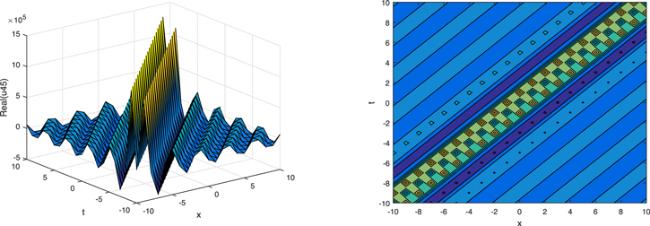
Figure 17. Graphical representation and corresponding contour of u45(x, t) for different values of parameters. |
The mixed singular solution is obtained as
$\begin{eqnarray*}\begin{array}{rcl}{u}_{46}(\xi ) & = & \displaystyle \frac{{\alpha }_{2}\left(-{\lambda }^{2}\right){p}^{4}{\mathrm{ln}}^{2}(B)-{cp}-{\alpha }_{3}{q}^{2}-{\alpha }_{3}{s}^{2}}{{\alpha }_{1}p}\\ & & -\displaystyle \frac{12{\alpha }_{2}\lambda {p}^{3}r{\mathrm{ln}}^{2}(B)}{{\alpha }_{1}(2p+1)}\\ & & \times \left(-\displaystyle \frac{\lambda }{2r}-\displaystyle \frac{\sqrt{-3{\lambda }^{2}}}{2r}\left({\coth }_{B}\left(\sqrt{3{\lambda }^{2}}\xi \right)\right.\right.\\ & & \left.\left.\pm \sqrt{({pq})}{{csch}}_{B}\left(\sqrt{3{\lambda }^{2}}\xi \right)\right)\Space{0ex}{3.5ex}{0ex}\right).\end{array}\end{eqnarray*}$
The plot and its corresponding contour plot of the solutions u46(x, t) are depicted in figure 18, for the values of parameters c = 20, p = 20, μ = 1.011, s = 1.05, α1 = 10, α2 = 10.9, α3 = 2, q = 10.2, q = 10.1, and B = 5.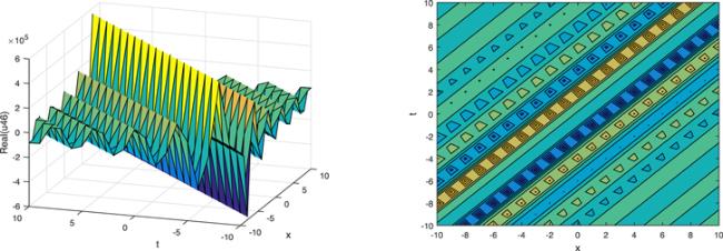
Figure 18. Graphical representation and corresponding contour of u46(x, t) for different values of parameters. |
The dark solution is obtained as
$\begin{eqnarray*}\begin{array}{rcl}{u}_{47}(\xi ) & = & \displaystyle \frac{{\alpha }_{2}\left(-{\lambda }^{2}\right){p}^{4}{\mathrm{ln}}^{2}(B)-{cp}-{\alpha }_{3}{q}^{2}-{\alpha }_{3}{s}^{2}}{{\alpha }_{1}p}\\ & & -\displaystyle \frac{12{\alpha }_{2}\lambda {p}^{3}r{\mathrm{ln}}^{2}(B)}{{\alpha }_{1}(2p+1)}\left(-\displaystyle \frac{\lambda }{2r}+\displaystyle \frac{\sqrt{3{\lambda }^{2}}}{4r}\right.\\ & & \left.\times \left({\tanh }_{B}\left(\displaystyle \frac{\sqrt{3{\lambda }^{2}}}{4}\xi \right)+{\coth }_{B}\left(\displaystyle \frac{\sqrt{3{\lambda }^{2}}}{4}\xi \right)\right)\right).\end{array}\end{eqnarray*}$
The plot and its corresponding contour plot of the solutions u47(x, t) are depicted in figure 19, for the values of parameters c = 20, p = 20, μ = 1.011, s = 1.05, α1 = 10, α2 = 10.9, α3 = 2, q = 10.2, q = 10.1, and B = 5.
Figure 19. Graphical representation and corresponding contour of u47(x, t) for different values of parameters. |
Type 3: For λ2 = μr we have trigonometric solutions obtained as
$\begin{eqnarray*}\begin{array}{rcl}{u}_{48}(\xi ) & = & \displaystyle \frac{{\alpha }_{2}\left(-{\lambda }^{2}\right){p}^{4}{\mathrm{ln}}^{2}(B)-{cp}-{\alpha }_{3}{q}^{2}-{\alpha }_{3}{s}^{2}}{{\alpha }_{1}p}\\ & & +\displaystyle \frac{12{\alpha }_{2}\lambda {p}^{3}r{\mathrm{ln}}^{2}(B)}{{\alpha }_{1}(2p+1)}\left(\displaystyle \frac{\lambda \mathrm{ln}(B)\xi +2}{\rho r\mathrm{ln}(B)}\right).\end{array}\end{eqnarray*}$
Type 4: For λ = χ, μ = νχ(ν ≠ 0) and r = 0 we have trigonometric solutions obtained as $\begin{eqnarray*}\begin{array}{rcl}{u}_{49}(\xi ) & = & \displaystyle \frac{{\alpha }_{2}\left(-{\lambda }^{2}\right){p}^{4}{\mathrm{ln}}^{2}(B)-{cp}-{\alpha }_{3}{q}^{2}-{\alpha }_{3}{s}^{2}}{{\alpha }_{1}p}\\ & & -\displaystyle \frac{12{\alpha }_{2}\lambda {p}^{3}r{\mathrm{ln}}^{2}(B)}{{\alpha }_{1}(2p+1)}\left({B}^{\chi \rho }-\nu \right).\end{array}\end{eqnarray*}$
Type 5: For λ = χ, r = νχ(ν ≠ 0) and μ = 0 we have obtained a plane solution as $\begin{eqnarray*}\begin{array}{rcl}{u}_{50}(\xi ) & = & \displaystyle \frac{{\alpha }_{2}\left(-{\lambda }^{2}\right){p}^{4}{\mathrm{ln}}^{2}(B)-{cp}-{\alpha }_{3}{q}^{2}-{\alpha }_{3}{s}^{2}}{{\alpha }_{1}p}\\ & & -\displaystyle \frac{12{\alpha }_{2}\lambda {p}^{3}r{\mathrm{ln}}^{2}(B)}{{\alpha }_{1}(2p+1)}\left(\displaystyle \frac{{{pB}}^{\chi \rho }}{p-\nu {{qB}}^{\chi \rho }}\right).\end{array}\end{eqnarray*}$
Type 6: For μ = 0, and λ ≠ 0 we obtained mixed hyperbolic solutions as $\begin{eqnarray*}\begin{array}{l}{u}_{51}(\xi )=\displaystyle \frac{{\alpha }_{2}\left(-{\lambda }^{2}\right){p}^{4}{\mathrm{ln}}^{2}(B)-{cp}-{\alpha }_{3}{q}^{2}-{\alpha }_{3}{s}^{2}}{{\alpha }_{1}p}\\ +\displaystyle \frac{12{\alpha }_{2}\lambda {p}^{3}r{\mathrm{ln}}^{2}(B)}{{\alpha }_{1}(2p+1)}\\ \left(\displaystyle \frac{p\tfrac{\sqrt{{\alpha }_{3}{q}^{2}+{\alpha }_{3}{s}^{2}}}{\sqrt{5}\sqrt{{\alpha }_{2}}{p}^{2}\mathrm{ln}(B)}}{r\left({\cosh }_{B}\left(\tfrac{\sqrt{{\alpha }_{3}{q}^{2}+{\alpha }_{3}{s}^{2}}}{\sqrt{5}\sqrt{{\alpha }_{2}}{p}^{2}\mathrm{ln}(B)}\xi \right)-{\sinh }_{B}\left(\tfrac{\sqrt{{\alpha }_{3}{q}^{2}+{\alpha }_{3}{s}^{2}}}{\sqrt{5}\sqrt{{\alpha }_{2}}{p}^{2}\mathrm{ln}(B)}\xi \right)+p\right)}\right).\end{array}\end{eqnarray*}$
The plot and its corresponding contour plot of the solutions u51(x, t) are depicted in figure 20, for the values of parameters c = 200, p = 20, μ = 100, s = 1.05, α1 = 100, α2 = 10.9, α3 = 2, q = 10.2, q = 10.1, and B = 5. $\begin{eqnarray*}\begin{array}{l}{u}_{52}(\xi )=\displaystyle \frac{{\alpha }_{2}\left(-{\lambda }^{2}\right){p}^{4}{\mathrm{ln}}^{2}(B)-{cp}-{\alpha }_{3}{q}^{2}-{\alpha }_{3}{s}^{2}}{{\alpha }_{1}p}\\ +\displaystyle \frac{12{\alpha }_{2}\lambda {p}^{3}r{\mathrm{ln}}^{2}(B)}{{\alpha }_{1}(2p+1)}\\ \left(\displaystyle \frac{p\tfrac{\sqrt{{\alpha }_{3}{q}^{2}+{\alpha }_{3}{s}^{2}}}{\sqrt{5}\sqrt{{\alpha }_{2}}{p}^{2}\mathrm{ln}(B)}\left({\sinh }_{B}\left(\tfrac{\sqrt{{\alpha }_{3}{q}^{2}+{\alpha }_{3}{s}^{2}}}{\sqrt{5}\sqrt{{\alpha }_{2}}{p}^{2}\mathrm{ln}(B)}\xi \right)+{\cosh }_{B}\left(\tfrac{\sqrt{{\alpha }_{3}{q}^{2}+{\alpha }_{3}{s}^{2}}}{\sqrt{5}\sqrt{{\alpha }_{2}}{p}^{2}\mathrm{ln}(B)}\xi \right)\right)}{r\left({\sinh }_{B}\left(\tfrac{\sqrt{{\alpha }_{3}{q}^{2}+{\alpha }_{3}{s}^{2}}}{\sqrt{5}\sqrt{{\alpha }_{2}}{p}^{2}\mathrm{ln}(B)}\xi \right)+{\cosh }_{B}\left(\tfrac{\sqrt{{\alpha }_{3}{q}^{2}+{\alpha }_{3}{s}^{2}}}{\sqrt{5}\sqrt{{\alpha }_{2}}{p}^{2}\mathrm{ln}(B)}\xi \right)+p\right)}\right).\end{array}\end{eqnarray*}$

Figure 20. Graphical representation and corresponding contour of u51(x, t) for different values of parameters. |
Case 3: Where free parameters are μ, r and λ while along with b0 = b0, ${b}_{1}=-\tfrac{\lambda \left({\alpha }_{1}{b}_{0}p+{\alpha }_{2}{\lambda }^{2}{p}^{4}{\mathrm{ln}}^{2}(B)+8{\alpha }_{2}\mu {p}^{4}r{\mathrm{ln}}^{2}(B)+{cp}+{\alpha }_{3}{q}^{2}+{\alpha }_{3}{s}^{2}\right)}{{\alpha }_{1}\mu {p}^{2}}$
Type 1:For λ2 − μr < 0 and r ≠ 0, the mixed trigonometric solutions are found as
$\begin{eqnarray*}\begin{array}{l}{u}_{53}(\xi )={b}_{0}\\ -\displaystyle \frac{\lambda \left({\alpha }_{1}{b}_{0}p+{\alpha }_{2}{\lambda }^{2}{p}^{4}{\mathrm{ln}}^{2}(B)+8{\alpha }_{2}\mu {p}^{4}r{\mathrm{ln}}^{2}(B)+{cp}+{\alpha }_{3}{q}^{2}+{\alpha }_{3}{s}^{2}\right)}{{\alpha }_{1}\mu {p}^{2}}\\ \times \left(-\displaystyle \frac{\lambda }{2r}+\displaystyle \frac{\sqrt{-({\lambda }^{2}-4\mu r)}}{2r}{\tan }_{B}\left(\displaystyle \frac{\sqrt{-({\lambda }^{2}-4\mu r)}}{2}\xi \right)\right),\end{array}\end{eqnarray*}$
$\begin{eqnarray*}\begin{array}{l}{u}_{54}(\xi )={b}_{0}\\ -\displaystyle \frac{\lambda \left({\alpha }_{1}{b}_{0}p+{\alpha }_{2}{\lambda }^{2}{p}^{4}{\mathrm{ln}}^{2}(B)+8{\alpha }_{2}\mu {p}^{4}r{\mathrm{ln}}^{2}(B)+{cp}+{\alpha }_{3}{q}^{2}+{\alpha }_{3}{s}^{2}\right)}{{\alpha }_{1}\mu {p}^{2}}\\ \times \left(-\displaystyle \frac{\lambda }{2r}-\displaystyle \frac{\sqrt{-({\lambda }^{2}-4\mu r)}}{2r}{\cot }_{B}\left(\displaystyle \frac{\sqrt{-({\lambda }^{2}-4\mu r)}}{2}\xi \right)\right),\end{array}\end{eqnarray*}$
$\begin{eqnarray*}\begin{array}{l}{u}_{55}(\xi )={b}_{0}-\displaystyle \frac{\lambda \left({\alpha }_{1}{b}_{0}p+{\alpha }_{2}{\lambda }^{2}{p}^{4}{\mathrm{ln}}^{2}(B)+8{\alpha }_{2}\mu {p}^{4}r{\mathrm{ln}}^{2}(B)+{cp}+{\alpha }_{3}{q}^{2}+{\alpha }_{3}{s}^{2}\right)}{{\alpha }_{1}\mu {p}^{2}}\\ \times \left(-\displaystyle \frac{\lambda }{2r}+\displaystyle \frac{\sqrt{-({\lambda }^{2}-4\mu r)}}{2r}\left({\tan }_{B}\left(\sqrt{-({\lambda }^{2}-4\mu r)}\xi \right)\right.\right.\\ \left.\left.\pm \sqrt{({pq})}{\sec }_{B}\left(\sqrt{-({\lambda }^{2}-4\mu r)}\xi \right)\right)\Space{0ex}{3.5ex}{0ex}\right).\end{array}\end{eqnarray*}$
The plot and its corresponding contour plot of the solutions u55(x, t) are depicted in figure 21, for the values of parameters c = 2, p = 2, μ = 0.011, s = 1.05, α1 = 1, α2 = 0.9, α3 = 2, q = 10.2, q = 10.1, and B = 5. $\begin{eqnarray*}\begin{array}{l}{u}_{56}(\xi )={b}_{0}\\ -\displaystyle \frac{\lambda \left({\alpha }_{1}{b}_{0}p+{\alpha }_{2}{\lambda }^{2}{p}^{4}{\mathrm{ln}}^{2}(B)+8{\alpha }_{2}\mu {p}^{4}r{\mathrm{ln}}^{2}(B)+{cp}+{\alpha }_{3}{q}^{2}+{\alpha }_{3}{s}^{2}\right)}{{\alpha }_{1}\mu {p}^{2}}\\ \times \left(-\displaystyle \frac{\lambda }{2r}-\displaystyle \frac{\sqrt{-({\lambda }^{2}-4\mu r)}}{2r}\left({\cot }_{B}\left(\sqrt{-({\lambda }^{2}-4\mu r)}\xi \right)\right.\right.\\ \left.\left.\pm \sqrt{({pq})}{\csc }_{B}\left(\sqrt{-({\lambda }^{2}-4\mu r)}\xi \right)\right)\Space{0ex}{3.5ex}{0ex}\right),\end{array}\end{eqnarray*}$
$\begin{eqnarray*}\begin{array}{l}{u}_{57}(\xi )={b}_{0}\\ -\displaystyle \frac{\lambda \left({\alpha }_{1}{b}_{0}p+{\alpha }_{2}{\lambda }^{2}{p}^{4}{\mathrm{ln}}^{2}(B)+8{\alpha }_{2}\mu {p}^{4}r{\mathrm{ln}}^{2}(B)+{cp}+{\alpha }_{3}{q}^{2}+{\alpha }_{3}{s}^{2}\right)}{{\alpha }_{1}\mu {p}^{2}}\\ \times \left(-\displaystyle \frac{\lambda }{2r}+\displaystyle \frac{\sqrt{-({\lambda }^{2}-4\mu r)}}{2r}\left({\tan }_{B}\left(\sqrt{-({\lambda }^{2}-4\mu r)}\xi \right)\right.\right.\\ \left.\left.-\sqrt{({pq})}{\cot }_{B}\left(\sqrt{-({\lambda }^{2}-4\mu r)}\xi \right)\right)\Space{0ex}{3.5ex}{0ex}\right).\end{array}\end{eqnarray*}$

Figure 21. Graphical representation and corresponding contour of u55(x, t) for different values of parameters. |
Type 2 For λ2 − μr > 0 and r ≠ 0, different types of solutions are obtained.
The dark solutions are obtained as
where ρ = ρ(x, y, z, t) and p, q > 0.
$\begin{eqnarray*}\begin{array}{l}{u}_{58}(\xi )={b}_{0}\\ -\displaystyle \frac{\lambda \left({\alpha }_{1}{b}_{0}p+{\alpha }_{2}{\lambda }^{2}{p}^{4}{\mathrm{ln}}^{2}(B)+8{\alpha }_{2}\mu {p}^{4}r{\mathrm{ln}}^{2}(B)+{cp}+{\alpha }_{3}{q}^{2}+{\alpha }_{3}{s}^{2}\right)}{{\alpha }_{1}\mu {p}^{2}}\\ \times \left(-\displaystyle \frac{\lambda }{2r}-\displaystyle \frac{\sqrt{-({\lambda }^{2}-4\mu r)}}{2r}{\tanh }_{B}\left(\displaystyle \frac{\sqrt{-({\lambda }^{2}-4\mu r)}}{2}\xi \right)\right),\end{array}\end{eqnarray*}$
The singular solution is obtained as $\begin{eqnarray*}\begin{array}{l}{u}_{59}(\xi )={b}_{0}\\ -\displaystyle \frac{\lambda \left({\alpha }_{1}{b}_{0}p+{\alpha }_{2}{\lambda }^{2}{p}^{4}{\mathrm{ln}}^{2}(B)+8{\alpha }_{2}\mu {p}^{4}r{\mathrm{ln}}^{2}(B)+{cp}+{\alpha }_{3}{q}^{2}+{\alpha }_{3}{s}^{2}\right)}{{\alpha }_{1}\mu {p}^{2}}\\ \times \left(-\displaystyle \frac{\lambda }{2r}-\displaystyle \frac{\sqrt{-({\lambda }^{2}-4\mu r)}}{2r}{\coth }_{B}\left(\displaystyle \frac{\sqrt{-({\lambda }^{2}-4\mu r)}}{2}\xi \right)\right).\end{array}\end{eqnarray*}$
The complex dark bright solution is obtained as $\begin{eqnarray*}\begin{array}{l}{u}_{60}(\xi )={b}_{0}\\ -\displaystyle \frac{\lambda \,\left({\alpha }_{1}{b}_{0}p+{\alpha }_{2}{\lambda }^{2}{p}^{4}{\mathrm{ln}}^{2}(B)+8{\alpha }_{2}\mu {p}^{4}r{\mathrm{ln}}^{2}(B)+{cp}+{\alpha }_{3}{q}^{2}+{\alpha }_{3}{s}^{2}\right)}{{\alpha }_{1}\mu {p}^{2}}\\ \times \left(-\displaystyle \frac{\lambda }{2r}-\displaystyle \frac{\sqrt{-({\lambda }^{2}-4\mu r)}}{2r}\left({\tanh }_{B}\left(\sqrt{3{\lambda }^{2}}\xi \right)\right.\right.\\ \left.\left.\pm {\rm{i}}\sqrt{({pq})}{{{\rm{sech}} }}_{B}\left(\sqrt{-({\lambda }^{2}-4\mu r)}\xi \right)\right)\Space{0ex}{3.5ex}{0ex}\right).\end{array}\end{eqnarray*}$
The mixed singular solution is obtained as $\begin{eqnarray*}\begin{array}{l}{u}_{61}(\xi )={b}_{0}\\ -\displaystyle \frac{\lambda \left({\alpha }_{1}{b}_{0}p+{\alpha }_{2}{\lambda }^{2}{p}^{4}{\mathrm{ln}}^{2}(B)+8{\alpha }_{2}\mu {p}^{4}r{\mathrm{ln}}^{2}(B)+{cp}+{\alpha }_{3}{q}^{2}+{\alpha }_{3}{s}^{2}\right)}{{\alpha }_{1}\mu {p}^{2}}\\ \times \left(-\displaystyle \frac{\lambda }{2r}-\displaystyle \frac{\sqrt{-({\lambda }^{2}-4\mu r)}}{2r}\left({\coth }_{B}\left(\sqrt{-({\lambda }^{2}-4\mu r)}\xi \right)\right.\right.\\ \left.\left.\pm \sqrt{({pq})}{{csch}}_{B}\left(\sqrt{3{\lambda }^{2}}\xi \right)\right)\Space{0ex}{3.5ex}{0ex}\right).\end{array}\end{eqnarray*}$
The dark solution is obtained as $\begin{eqnarray*}\begin{array}{l}{u}_{62}(\xi )={b}_{0}\\ -\displaystyle \frac{\lambda \left({\alpha }_{1}{b}_{0}p+{\alpha }_{2}{\lambda }^{2}{p}^{4}{\mathrm{ln}}^{2}(B)+8{\alpha }_{2}\mu {p}^{4}r{\mathrm{ln}}^{2}(B)+{cp}+{\alpha }_{3}{q}^{2}+{\alpha }_{3}{s}^{2}\right)}{{\alpha }_{1}\mu {p}^{2}}\\ \times \left(-\displaystyle \frac{\lambda }{2r}+\displaystyle \frac{\sqrt{-({\lambda }^{2}-4\mu r)}}{4r}\left({\tanh }_{B}\left(\displaystyle \frac{\sqrt{3{\lambda }^{2}}}{4}\xi \right)\right.\right.\\ \left.\left.+{\coth }_{B}\left(\displaystyle \frac{\sqrt{-({\lambda }^{2}-4\mu r)}}{4}\xi \right)\right)\right).\end{array}\end{eqnarray*}$
Type 3: For μr > 0 and λ = 0, we obtained trigonometric solutions as $\begin{eqnarray*}\begin{array}{l}{u}_{63}(\xi )={b}_{0}\\ -\displaystyle \frac{\lambda \left({\alpha }_{1}{b}_{0}p+{\alpha }_{2}{\lambda }^{2}{p}^{4}{\mathrm{ln}}^{2}(B)+8{\alpha }_{2}\mu {p}^{4}r{\mathrm{ln}}^{2}(B)+{cp}+{\alpha }_{3}{q}^{2}+{\alpha }_{3}{s}^{2}\right)}{{\alpha }_{1}\mu {p}^{2}}\\ \times \left(\sqrt{\displaystyle \frac{\mu }{r}}{\tan }_{B}(\sqrt{\mu r}\xi )\right),\end{array}\end{eqnarray*}$
$\begin{eqnarray*}\begin{array}{l}{u}_{64}(\xi )={b}_{0}\\ -\displaystyle \frac{\lambda \left({\alpha }_{1}{b}_{0}p+{\alpha }_{2}{\lambda }^{2}{p}^{4}{\mathrm{ln}}^{2}(B)+8{\alpha }_{2}\mu {p}^{4}r{\mathrm{ln}}^{2}(B)+{cp}+{\alpha }_{3}{q}^{2}+{\alpha }_{3}{s}^{2}\right)}{{\alpha }_{1}\mu {p}^{2}}\\ \times \left(\sqrt{\displaystyle \frac{\mu }{r}}{\cot }_{B}(\sqrt{\mu r}\xi )\right),\end{array}\end{eqnarray*}$
The mixed trigonometric solutions were obtained as $\begin{eqnarray*}\begin{array}{l}{u}_{65}(\xi )={b}_{0}\\ -\displaystyle \frac{\lambda \left({\alpha }_{1}{b}_{0}p+{\alpha }_{2}{\lambda }^{2}{p}^{4}{\mathrm{ln}}^{2}(B)+8{\alpha }_{2}\mu {p}^{4}r{\mathrm{ln}}^{2}(B)+{cp}+{\alpha }_{3}{q}^{2}+{\alpha }_{3}{s}^{2}\right)}{{\alpha }_{1}\mu {p}^{2}}\\ \times \left(\sqrt{\displaystyle \frac{\mu }{r}}\left({\tan }_{B}(2\sqrt{\mu r}\xi )\pm \sqrt{{pq}}{\sec }_{B}(2\sqrt{\mu r}\xi )\right)\right),\end{array}\end{eqnarray*}$
$\begin{eqnarray*}\begin{array}{l}{u}_{66}(\xi )={b}_{0}\\ -\displaystyle \frac{\lambda \left({\alpha }_{1}{b}_{0}p+{\alpha }_{2}{\lambda }^{2}{p}^{4}{\mathrm{ln}}^{2}(B)+8{\alpha }_{2}\mu {p}^{4}r{\mathrm{ln}}^{2}(B)+{cp}+{\alpha }_{3}{q}^{2}+{\alpha }_{3}{s}^{2}\right)}{{\alpha }_{1}\mu {p}^{2}}\\ \times \left(\sqrt{\displaystyle \frac{\mu }{r}}\left({\cot }_{B}(2\sqrt{\mu r}\xi )\pm \sqrt{{pq}}{\csc }_{B}(2\sqrt{\mu r}\xi )\right)\right),\end{array}\end{eqnarray*}$
$\begin{eqnarray*}\begin{array}{l}{u}_{67}(\xi )={b}_{0}\\ -\displaystyle \frac{\lambda \left({\alpha }_{1}{b}_{0}p+{\alpha }_{2}{\lambda }^{2}{p}^{4}{\mathrm{ln}}^{2}(B)+8{\alpha }_{2}\mu {p}^{4}r{\mathrm{ln}}^{2}(B)+{cp}+{\alpha }_{3}{q}^{2}+{\alpha }_{3}{s}^{2}\right)}{{\alpha }_{1}\mu {p}^{2}}\\ \times \displaystyle \frac{1}{2}\sqrt{\displaystyle \frac{\mu }{r}}\left({\tan }_{B}(\displaystyle \frac{\sqrt{\mu r}}{2}\xi )-\sqrt{{pq}}{\cot }_{B}(\displaystyle \frac{\sqrt{\mu r}}{2}\xi )\right).\end{array}\end{eqnarray*}$
Type 4: For μr < 0 and λ = 0, we obtained dark solutions as $\begin{eqnarray*}\begin{array}{l}{u}_{68}(\xi )={b}_{0}\\ -\displaystyle \frac{\lambda \left({\alpha }_{1}{b}_{0}p+{\alpha }_{2}{\lambda }^{2}{p}^{4}{\mathrm{ln}}^{2}(B)+8{\alpha }_{2}\mu {p}^{4}r{\mathrm{ln}}^{2}(B)+{cp}+{\alpha }_{3}{q}^{2}+{\alpha }_{3}{s}^{2}\right)}{{\alpha }_{1}\mu {p}^{2}}\\ \times \left(\sqrt{-\displaystyle \frac{\mu }{r}}{\tanh }_{B}(\sqrt{-\mu r}\xi )\right),\end{array}\end{eqnarray*}$
We get the singular solution as $\begin{eqnarray*}\begin{array}{l}{u}_{69}(\xi )={b}_{0}\\ -\displaystyle \frac{\lambda \left({\alpha }_{1}{b}_{0}p+{\alpha }_{2}{\lambda }^{2}{p}^{4}{\mathrm{ln}}^{2}(B)+8{\alpha }_{2}\mu {p}^{4}r{\mathrm{ln}}^{2}(B)+{cp}+{\alpha }_{3}{q}^{2}+{\alpha }_{3}{s}^{2}\right)}{{\alpha }_{1}\mu {p}^{2}}\\ \times \left(\sqrt{-\displaystyle \frac{\mu }{r}}{\coth }_{B}(\sqrt{-\mu r}\xi )\right),\end{array}\end{eqnarray*}$
The different type of complex combo solutions are obtained as $\begin{eqnarray*}\begin{array}{l}{u}_{70}(\xi )={b}_{0}\\ -\displaystyle \frac{\lambda \left({\alpha }_{1}{b}_{0}p+{\alpha }_{2}{\lambda }^{2}{p}^{4}{\mathrm{ln}}^{2}(B)+8{\alpha }_{2}\mu {p}^{4}r{\mathrm{ln}}^{2}(B)+{cp}+{\alpha }_{3}{q}^{2}+{\alpha }_{3}{s}^{2}\right)}{{\alpha }_{1}\mu {p}^{2}}\\ \times \sqrt{-\displaystyle \frac{\mu }{r}}\left({\tanh }_{B}(2\sqrt{-\mu r}\xi )\right.\\ \left.\pm {\rm{i}}\sqrt{{pq}}{{\rm{{\rm{sech}} }}}_{B}(2\sqrt{-\mu r}\xi \right),\end{array}\end{eqnarray*}$
$\begin{eqnarray*}\begin{array}{l}{u}_{71}(\xi )={b}_{0}\\ -\displaystyle \frac{\lambda \left({\alpha }_{1}{b}_{0}p+{\alpha }_{2}{\lambda }^{2}{p}^{4}{\mathrm{ln}}^{2}(B)+8{\alpha }_{2}\mu {p}^{4}r{\mathrm{ln}}^{2}(B)+{cp}+{\alpha }_{3}{q}^{2}+{\alpha }_{3}{s}^{2}\right)}{{\alpha }_{1}\mu {p}^{2}}\\ \times \sqrt{-\displaystyle \frac{\mu }{r}}\left({\coth }_{B}(2\sqrt{-\mu r}\xi )\right.\\ \left.\pm \sqrt{{pq}}{{\rm{csch}}}_{B}(2\sqrt{-\mu r}\xi \right),\end{array}\end{eqnarray*}$
$\begin{eqnarray*}\begin{array}{l}{u}_{72}(\xi )={b}_{0}\\ -\displaystyle \frac{\lambda \left({\alpha }_{1}{b}_{0}p+{\alpha }_{2}{\lambda }^{2}{p}^{4}{\mathrm{ln}}^{2}(B)+8{\alpha }_{2}\mu {p}^{4}r{\mathrm{ln}}^{2}(B)+{cp}+{\alpha }_{3}{q}^{2}+{\alpha }_{3}{s}^{2}\right)}{{\alpha }_{1}\mu {p}^{2}}\\ \times \displaystyle \frac{1}{2}\sqrt{\displaystyle \frac{-\mu }{r}}\left({\tanh }_{B}(\displaystyle \frac{\sqrt{-\mu r}}{2}\xi )-{\coth }_{B}(\displaystyle \frac{\sqrt{-\mu r}}{2}\xi )\right).\end{array}\end{eqnarray*}$
Type 5: For λ = 0 and μ = r, the periodic and mixed periodic solutions are obtained as $\begin{eqnarray*}\begin{array}{l}{u}_{73}(\xi )={b}_{0}\\ -\displaystyle \frac{\lambda \left({\alpha }_{1}{b}_{0}p+{\alpha }_{2}{\lambda }^{2}{p}^{4}{\mathrm{ln}}^{2}(B)+8{\alpha }_{2}\mu {p}^{4}r{\mathrm{ln}}^{2}(B)+{cp}+{\alpha }_{3}{q}^{2}+{\alpha }_{3}{s}^{2}\right)}{{\alpha }_{1}\mu {p}^{2}}\\ \times \left({\tan }_{B}(\mu \xi )\right),\end{array}\end{eqnarray*}$
$\begin{eqnarray*}\begin{array}{l}{u}_{74}(\xi )={b}_{0}\\ -\displaystyle \frac{\lambda \left({\alpha }_{1}{b}_{0}p+{\alpha }_{2}{\lambda }^{2}{p}^{4}{\mathrm{ln}}^{2}(B)+8{\alpha }_{2}\mu {p}^{4}r{\mathrm{ln}}^{2}(B)+{cp}+{\alpha }_{3}{q}^{2}+{\alpha }_{3}{s}^{2}\right)}{{\alpha }_{1}\mu {p}^{2}}\\ \times \left(-{\cot }_{B}(\mu \xi )\right),\end{array}\end{eqnarray*}$
$\begin{eqnarray*}\begin{array}{l}{u}_{75}(\xi )={b}_{0}\\ -\displaystyle \frac{\lambda \left({\alpha }_{1}{b}_{0}p+{\alpha }_{2}{\lambda }^{2}{p}^{4}{\mathrm{ln}}^{2}(B)+8{\alpha }_{2}\mu {p}^{4}r{\mathrm{ln}}^{2}(B)+{cp}+{\alpha }_{3}{q}^{2}+{\alpha }_{3}{s}^{2}\right)}{{\alpha }_{1}\mu {p}^{2}}\\ \times \left({\tan }_{B}(2\mu \xi )\pm \sqrt{{pq}}{\sec }_{B}(2\mu \xi )\right),\end{array}\end{eqnarray*}$
$\begin{eqnarray*}\begin{array}{l}{u}_{76}(\xi )={b}_{0}\\ -\displaystyle \frac{\lambda \left({\alpha }_{1}{b}_{0}p+{\alpha }_{2}{\lambda }^{2}{p}^{4}{\mathrm{ln}}^{2}(B)+8{\alpha }_{2}\mu {p}^{4}r{\mathrm{ln}}^{2}(B)+{cp}+{\alpha }_{3}{q}^{2}+{\alpha }_{3}{s}^{2}\right)}{{\alpha }_{1}\mu {p}^{2}}\\ \times \left({\cot }_{B}(2\mu \xi )\pm \sqrt{{pq}}{{\rm{\csc }}}_{B}(2\mu \xi )\right),\end{array}\end{eqnarray*}$
$\begin{eqnarray*}\begin{array}{l}{u}_{77}(\xi )={b}_{0}\\ -\displaystyle \frac{\lambda \left({\alpha }_{1}{b}_{0}p+{\alpha }_{2}{\lambda }^{2}{p}^{4}{\mathrm{ln}}^{2}(B)+8{\alpha }_{2}\mu {p}^{4}r{\mathrm{ln}}^{2}(B)+{cp}+{\alpha }_{3}{q}^{2}+{\alpha }_{3}{s}^{2}\right)}{{\alpha }_{1}\mu {p}^{2}}\\ \times \displaystyle \frac{1}{2}\left({\tan }_{B}(\displaystyle \frac{\sqrt{\mu }}{2}\xi )-{\cot }_{B}(\displaystyle \frac{\mu }{2}\xi )\right).\end{array}\end{eqnarray*}$
Type 6: For λ = 0 and r = −μ, we obtained different types of solutions as $\begin{eqnarray*}\begin{array}{l}{u}_{78}(\xi )={b}_{0}\\ -\displaystyle \frac{\lambda \left({\alpha }_{1}{b}_{0}p+{\alpha }_{2}{\lambda }^{2}{p}^{4}{\mathrm{ln}}^{2}(B)+8{\alpha }_{2}\mu {p}^{4}r{\mathrm{ln}}^{2}(B)+{cp}+{\alpha }_{3}{q}^{2}+{\alpha }_{3}{s}^{2}\right)}{{\alpha }_{1}\mu {p}^{2}}\\ \times \left({\tanh }_{B}(\mu \xi )\right),\end{array}\end{eqnarray*}$
$\begin{eqnarray*}\begin{array}{l}{u}_{79}(\xi )={b}_{0}\\ -\displaystyle \frac{\lambda \left({\alpha }_{1}{b}_{0}p+{\alpha }_{2}{\lambda }^{2}{p}^{4}{\mathrm{ln}}^{2}(B)+8{\alpha }_{2}\mu {p}^{4}r{\mathrm{ln}}^{2}(B)+{cp}+{\alpha }_{3}{q}^{2}+{\alpha }_{3}{s}^{2}\right)}{{\alpha }_{1}\mu {p}^{2}}\\ \times \left({\coth }_{B}(\mu \xi )\right),\end{array}\end{eqnarray*}$
$\begin{eqnarray*}\begin{array}{l}{u}_{80}(\xi )={b}_{0}\\ -\displaystyle \frac{\lambda \left({\alpha }_{1}{b}_{0}p+{\alpha }_{2}{\lambda }^{2}{p}^{4}{\mathrm{ln}}^{2}(B)+8{\alpha }_{2}\mu {p}^{4}r{\mathrm{ln}}^{2}(B)+{cp}+{\alpha }_{3}{q}^{2}+{\alpha }_{3}{s}^{2}\right)}{{\alpha }_{1}\mu {p}^{2}}\\ \times \left({\tanh }_{B}(2\mu \xi )\pm {\rm{i}}\sqrt{{pq}}{{\rm{{\rm{sech}} }}}_{B}(2\mu \xi )\right),\end{array}\end{eqnarray*}$
$\begin{eqnarray*}\begin{array}{l}{u}_{81}(\xi )={b}_{0}\\ -\displaystyle \frac{\lambda \left({\alpha }_{1}{b}_{0}p+{\alpha }_{2}{\lambda }^{2}{p}^{4}{\mathrm{ln}}^{2}(B)+8{\alpha }_{2}\mu {p}^{4}r{\mathrm{ln}}^{2}(B)+{cp}+{\alpha }_{3}{q}^{2}+{\alpha }_{3}{s}^{2}\right)}{{\alpha }_{1}\mu {p}^{2}}\\ \times \left({\coth }_{B}(2\mu \xi )\pm \sqrt{{pq}}{{\rm{csch}}}_{B}(2\mu \xi )\right),\end{array}\end{eqnarray*}$
$\begin{eqnarray*}\begin{array}{l}{u}_{82}(\xi )={b}_{0}\\ -\displaystyle \frac{\lambda \left({\alpha }_{1}{b}_{0}p+{\alpha }_{2}{\lambda }^{2}{p}^{4}{\mathrm{ln}}^{2}(B)+8{\alpha }_{2}\mu {p}^{4}r{\mathrm{ln}}^{2}(B)+{cp}+{\alpha }_{3}{q}^{2}+{\alpha }_{3}{s}^{2}\right)}{{\alpha }_{1}\mu {p}^{2}}\\ \times \displaystyle \frac{1}{2}\left({\tanh }_{B}(\displaystyle \frac{\sqrt{\mu }}{2}\xi )+{\coth }_{B}(\displaystyle \frac{\mu }{2}\xi )\right).\end{array}\end{eqnarray*}$
Type 7: For λ2 = 4μr we obtained only one solutions as $\begin{eqnarray*}\begin{array}{l}{u}_{83}(\xi )={b}_{0}\\ -\displaystyle \frac{\lambda \left({\alpha }_{1}{b}_{0}p+{\alpha }_{2}{\lambda }^{2}{p}^{4}{\mathrm{ln}}^{2}(B)+8{\alpha }_{2}\mu {p}^{4}r{\mathrm{ln}}^{2}(B)+{cp}+{\alpha }_{3}{q}^{2}+{\alpha }_{3}{s}^{2}\right)}{{\alpha }_{1}\mu {p}^{2}}\\ \times \left(\displaystyle \frac{2\mu \left(\left(\tfrac{\sqrt{{\alpha }_{3}{q}^{2}+{\alpha }_{3}{s}^{2}}}{\sqrt{5}\sqrt{{\alpha }_{2}}{p}^{2}}\right)\xi +2\right)}{\tfrac{{\alpha }_{3}({q}^{2}+{s}^{2})}{5{\alpha }_{2}{p}^{4}\mathrm{ln}(B)}\xi }\right).\end{array}\end{eqnarray*}$
Type 8: For λ = χ, μ = νχ(ν ≠ 0) and r = 0, we obtained only one solution as $\begin{eqnarray*}\begin{array}{l}{u}_{84}(\xi )={b}_{0}\\ -\displaystyle \frac{\lambda \left({\alpha }_{1}{b}_{0}p+{\alpha }_{2}{\lambda }^{2}{p}^{4}{\mathrm{ln}}^{2}(B)+8{\alpha }_{2}\mu {p}^{4}r{\mathrm{ln}}^{2}(B)+{cp}+{\alpha }_{3}{q}^{2}+{\alpha }_{3}{s}^{2}\right)}{{\alpha }_{1}\mu {p}^{2}}\\ \left({B}^{\chi \xi }-\nu \right).\end{array}\end{eqnarray*}$
Type 9: For λ = r = 0, we obtained only one solution as $\begin{eqnarray*}\begin{array}{l}{u}_{85}(\xi )=-{b}_{0}\\ -\displaystyle \frac{\lambda \left({\alpha }_{1}{b}_{0}p+{\alpha }_{2}{\lambda }^{2}{p}^{4}{\mathrm{ln}}^{2}(B)+8{\alpha }_{2}\mu {p}^{4}r{\mathrm{ln}}^{2}(B)+{cp}+{\alpha }_{3}{q}^{2}+{\alpha }_{3}{s}^{2}\right)}{{\alpha }_{1}\mu {p}^{2}}\\ \left(\mu \xi \mathrm{ln}(B)\right).\end{array}\end{eqnarray*}$
Type 10: For λ = μ = 0, we obtained only one solution as $\begin{eqnarray*}\begin{array}{l}{u}_{86}(\xi )={b}_{0}\\ -\displaystyle \frac{\lambda \left({\alpha }_{1}{b}_{0}p+{\alpha }_{2}{\lambda }^{2}{p}^{4}{\mathrm{ln}}^{2}(B)+8{\alpha }_{2}\mu {p}^{4}r{\mathrm{ln}}^{2}(B)+{cp}+{\alpha }_{3}{q}^{2}+{\alpha }_{3}{s}^{2}\right)}{{\alpha }_{1}\mu {p}^{2}}\\ \left(\displaystyle \frac{1}{r\xi \mathrm{ln}(B)}\right).\end{array}\end{eqnarray*}$
Type 11: For μ = 0, and λ ≠ 0 we obtained mixed hyperbolic solutions as $\begin{eqnarray*}\begin{array}{l}{u}_{87}(\xi )={b}_{0}\\ -\displaystyle \frac{\lambda \left({\alpha }_{1}{b}_{0}p+{\alpha }_{2}{\lambda }^{2}{p}^{4}{\mathrm{ln}}^{2}(B)+8{\alpha }_{2}\mu {p}^{4}r{\mathrm{ln}}^{2}(B)+{cp}+{\alpha }_{3}{q}^{2}+{\alpha }_{3}{s}^{2}\right)}{{\alpha }_{1}\mu {p}^{2}}\\ \times \left(\displaystyle \frac{p\tfrac{\sqrt{{\alpha }_{3}{q}^{2}+{\alpha }_{3}{s}^{2}}}{\sqrt{5}\sqrt{{\alpha }_{2}}{p}^{2}\mathrm{ln}(B)}}{r\left({\cosh }_{B}\left(\tfrac{\sqrt{{\alpha }_{3}{q}^{2}+{\alpha }_{3}{s}^{2}}}{\sqrt{5}\sqrt{{\alpha }_{2}}{p}^{2}\mathrm{ln}(B)}\xi \right)-{\sinh }_{B}\left(\tfrac{\sqrt{{\alpha }_{3}{q}^{2}+{\alpha }_{3}{s}^{2}}}{\sqrt{5}\sqrt{{\alpha }_{2}}{p}^{2}\mathrm{ln}(B)}\xi \right)+p\right)}\right).\end{array}\end{eqnarray*}$
$\begin{eqnarray*}\begin{array}{l}{u}_{88}(\xi )={b}_{0}\\ -\displaystyle \frac{\lambda \left({\alpha }_{1}{b}_{0}p+{\alpha }_{2}{\lambda }^{2}{p}^{4}{\mathrm{ln}}^{2}(B)+8{\alpha }_{2}\mu {p}^{4}r{\mathrm{ln}}^{2}(B)+{cp}+{\alpha }_{3}{q}^{2}+{\alpha }_{3}{s}^{2}\right)}{{\alpha }_{1}\mu {p}^{2}}\\ \times \left(\displaystyle \frac{p\tfrac{\sqrt{{\alpha }_{3}{q}^{2}+{\alpha }_{3}{s}^{2}}}{\sqrt{5}\sqrt{{\alpha }_{2}}{p}^{2}\mathrm{ln}(B)}\left({\sinh }_{B}\left(\tfrac{\sqrt{{\alpha }_{3}{q}^{2}+{\alpha }_{3}{s}^{2}}}{\sqrt{5}\sqrt{{\alpha }_{2}}{p}^{2}\mathrm{ln}(B)}\xi \right)+{\cosh }_{B}\left(\tfrac{\sqrt{{\alpha }_{3}{q}^{2}+{\alpha }_{3}{s}^{2}}}{\sqrt{5}\sqrt{{\alpha }_{2}}{p}^{2}\mathrm{ln}(B)}\xi \right)\right)}{r\left({\sinh }_{B}\left(\tfrac{\sqrt{{\alpha }_{3}{q}^{2}+{\alpha }_{3}{s}^{2}}}{\sqrt{5}\sqrt{{\alpha }_{2}}{p}^{2}\mathrm{ln}(B)}\xi \right)+{\cosh }_{B}\left(\tfrac{\sqrt{{\alpha }_{3}{q}^{2}+{\alpha }_{3}{s}^{2}}}{\sqrt{5}\sqrt{{\alpha }_{2}}{p}^{2}\mathrm{ln}(B)}\xi \right)+p\right)}\right).\end{array}\end{eqnarray*}$
Type 12: For λ = χ, r = νχ(ν ≠ 0) and μ = 0, we obtained a plane solution as $\begin{eqnarray*}\begin{array}{l}{u}_{89}(\xi )={b}_{0}\\ -\displaystyle \frac{\lambda \left({\alpha }_{1}{b}_{0}p+{\alpha }_{2}{\lambda }^{2}{p}^{4}{\mathrm{ln}}^{2}(B)+8{\alpha }_{2}\mu {p}^{4}r{\mathrm{ln}}^{2}(B)+{cp}+{\alpha }_{3}{q}^{2}+{\alpha }_{3}{s}^{2}\right)}{{\alpha }_{1}\mu {p}^{2}}\\ \left(\displaystyle \frac{{{pB}}^{\chi \xi }}{p-\nu {{qB}}^{\chi \xi }}\right).\end{array}\end{eqnarray*}$
In the all above solutions, the generalized hyperbolic and trigonometric functions are defined as| ${\sinh }_{B}(\rho )$ | $\tfrac{{{pB}}^{\rho }-{{qB}}^{-\rho }}{2}$ | ${\cosh }_{B}(\rho )$ | $\tfrac{{{pB}}^{\rho }+{{qB}}^{-\rho }}{2}$ |
| ${\tanh }_{B}(\rho )$ | $\tfrac{{{pB}}^{\rho }-{{qB}}^{-\rho }}{{{pB}}^{\rho }+{{qB}}^{-\rho }}$ | ${\coth }_{B}(\rho )$ | $\tfrac{{{pB}}^{\rho }+{{qB}}^{-\rho }}{{{pB}}^{\rho }-{{qB}}^{-\rho }}$ |
| ${\sin }_{B}(\rho )$ | $\tfrac{{{pB}}^{{\rm{i}}\rho }-{{qB}}^{-{\rm{i}}\rho }}{2}$ | ${\cos }_{B}(\rho )$ | $\tfrac{{{pB}}^{{\rm{i}}\rho }+{{qB}}^{-{\rm{i}}\rho }}{2}$ |
| ${\cot }_{B}(\rho )$ | $-{\rm{i}}\tfrac{{{pB}}^{{\rm{i}}\rho }-{{qB}}^{-{\rm{i}}\rho }}{{{pB}}^{{\rm{i}}\rho }+{{qB}}^{-{\rm{i}}\rho }}$ | ${\cot }_{B}(\rho )$ | $i\tfrac{{{pB}}^{{\rm{i}}\rho }+{{qB}}^{-{\rm{i}}\rho }}{{{pB}}^{{\rm{i}}\rho }-{{qB}}^{-{\rm{i}}\rho }}$ |
3. Conclusion
In this work, the (3 + 1)-dimensional fractional time-space KP (FTSKP) equation is under investigation, which propagates the acoustic waves in an unmagnetized dusty plasma. This fractional model is defined using the confirmable fractional derivatives. The diverse new families of hyperbolic, trigonometric, rational, and plane wave solutions are obtained in single and different combinations using the new modified extended direct algebraic (MEDA) technique. Graphical representations of the obtained results are also depicted with different choices of parameters.