


1. Introduction
Table 1. The definitions of variables. |
| Notations | |
|---|---|
| Symbol | Definition |
| ${\mathop{o}\limits^{\wedge }}_{1},{\mathop{o}\limits^{\wedge }}_{2}$ | Convex hull |
| ${O}_{1},{O}_{2}$ | Object |
| $S$ | Point set |
| $P,{P}^{{\prime} }$ | Convex polygon |
| ${P}_{1},{P}_{2},{P}_{3},{P}_{4},{P}_{i}$ | Convex hull point |
| $N$ | Data size |
| $M$ | Solution number |
| $\tilde{N},\tilde{M}$ | Sample data size and solutions |
| P(x),$\tilde{P}(x)$ | Cumulative distribution function |
| ϵ | failure rate |
| ${v}_{0},{v}_{1}$ | Coordinate values |
| Convex hull point | |
| $k$ | A copy to store convex hull point values |
| ${M}_{p}$ | The number of convex hull point |
2. Related works
2.1. Definition of convex hull and classic algorithm
| i | (i)The convex hull of the point set S in the n-dimensional space is the union of the convex combination of all $n+1$ points in the point set S. For example, in a two-dimensional space, the convex hull of a point set S is the union of all triangles covered by any three vertices in S. |
| ii | (ii)The convex hull of the point set S is the intersection of all convex sets containing S. |
| iii | (iii)The convex hull of the point set S is the intersection of all half spaces containing S. |
| iv | (iv)The convex hull of a point set S containing a finite number of points on the plane is the smallest convex polygon P containing S. The smallest meaning is that there is no polygon P′, making $P\supseteq P^{\prime} \supseteq S.$ |
| v | (v)The convex hull of a point set S containing a finite number of points on the plane is a convex polygon with the smallest area on the plane containing these points. |
| vi | (vi)The convex hull of a point set S containing a finite number of points on the plane is a convex polygon with the smallest perimeter surrounding these points on the plane. |
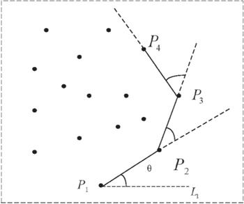
Figure 1. Gift wrapping algorithm. |
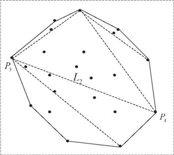
Figure 2. Quick sort algorithm. |
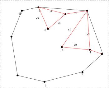
Figure 3. Graham algorithm. |
2.2. Quantum maximum or minimum searching algorithm
Randomly choose a data value from D as the reference value ${d}_{0}.$
Map D to the initial state $\left|\psi \right\rangle .$
Exploit quantum searching algorithm and obtain its result ${d}_{1},$ a data value of D.
If ${d}_{1}\leqslant {d}_{0},$ quantum searching algorithm is performed successfully, then update ${d}_{0}$ with ${d}_{1}$ as a new reference value. Otherwise, repeat steps 2–3.
Repeat steps 2–4.
3. Quantum convex hull algorithm (QCHA)
3.1. Quantum representation of point set
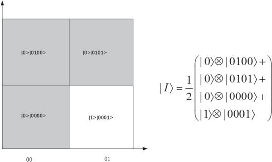
Figure 4. A 2 × 2 point set image, and it's NEQR representation, in which the white square represents a point. |
3.2. Design of QCHA
Randomly select a point and record its X-axis coordinate as ${v}_{0}.$
Map the points in the point concentration to the initial state $\left|I\right\rangle =\displaystyle \frac{1}{{2}^{G}}\displaystyle {\sum }_{Y=0}^{{2}^{G}}\displaystyle {\sum }_{X=0}^{{2}^{G}-1}\left|1\right\rangle \left|\left.YX\right\rangle \,\right..$
Use Grover–Long search algorithm to search, measure a piece of data ${v}_{1}.$
If ${v}_{1}$ < ${v}_{0},$ the retrieval is successful, then ${v}_{0}$ = ${v}_{1},$ otherwise repeat the second and third steps.
Repeat steps 2–4 (loop ${\mathrm{log}}_{2}n+c$ times then break).
The point ${p}_{0}$ that corresponds the minimum value ${v}_{0}$ is the extreme point.
Convert the scatter graph stored in classical information into a quantum state by NEQR model.
Use the minimum search algorithm to find the point ${p}_{0}$ with the smallest coordinate in the point set, that is, one of the points on the convex hull.
Copy ${p}_{0}$ to k.
Take point ${p}_{0}$ as the input value to enter C for iteration operation, find the next point ${p}_{1}$ of the convex hull edge and store it in the register, and judge whether ${p}_{1}$ and k are the same point, if they are equal, jump out of the whole step, otherwise assign ${p}_{1}$ to ${p}_{0}$ then continue the loop.
Read the value in the register, and the edge composed of its sequence is the convex hull.
3.3. Design of operation C
4. Simulation and time complexity analysis
4.1. Simulation
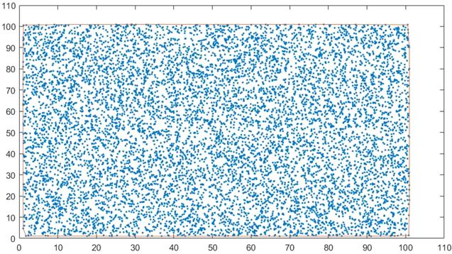
Figure 5. The simulation of QCHA. |
4.2. Time complexity analysis
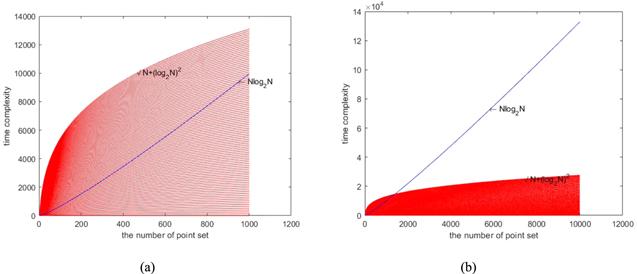
Figure 6. (a) The red line represents the change of ${M}_{p}\left(\sqrt{N}+{({\mathrm{log}}_{2}N)}^{2}\right)$ with ${M}_{p}$ from with 0 to 100, blue line is $N{\mathrm{log}}_{2}N.$ (b) M = 100, The maximum number of database points is 10 000. |