


1. Introduction
Plasmas considered as 'the most abundant form of ordinary matter in the Universe' have been observed to be associated with stars which extends to the rarefied intra-cluster medium and possibly the intergalactic regions [1]. For instance, the authors in [1] for various types of the cosmic dusty plasmas, considered an observationally/ experimentally-supported (3+1)-dimensional generalized variable-coefficient Kadomtsev–Petviashvili (KP)-Burgers-type equation. This equation could depict the dust-magneto-acoustic, dust-acoustic, magneto-acoustic, positron-acoustic, ion-acoustic, ion, electron-acoustic, quantum-dust-ion-acoustic or dust-ion-acoustic waves in one of the cosmic/laboratory dusty plasmas.
In recent years, the investigation of analytic travelling wave solutions of nonlinear partial differential equations (NPDEs) has been the concern of researchers who are involved in carrying out studies on the way to secure closed-form solutions of NPDEs that evolve from nonlinear phenomena [2–6]. These phenomena can be found in numerous fields of research including structured or methodical works in chemical kinematics, optical fibres, engineering, solid-state physics, oceanic, biology as well as meteorology [7–13]. In [14], Zakharov–Kuznetsov equation that delineates the ion-acoustic bob solitary waves present in an electron–positron–ion magneto-plasma arising in plasma physics was revealed. Moreover, double dispersion equations describing long nonlinear wave evolution in a thin hyper-elastic rod which apply in nonlinear science are divulged in [15]. The list continues. See more example [16–22].
As highlighted in [23], it is challenging to give a detailed and accurate definition of a soliton. Nevertheless, one can relate the term to any solution of NPDEs which stands for a wave of permanent form and also localized, such that it decays or better still approaches a constant at infinity and can as well establish a connection with other solitons that conserve its identity. It is well known that the soliton phenomena was first observed in the year 1834 [24]. Due to its relevance, securing soliton solutions of NPDEs has become a very important point of interest and an active research area for scientists [3, 4]. In particular, it has been revealed that soliton solutions are most remarkable when it comes to the study of nonlinear physical sciences. For instance, the wave phenomena which has been observed in high-energy physics, biophysics, fluid mechanics, chemical kinematics as well as in optical fibres [25]. Nonetheless, nonlinear processes are not easy to control and have surfaced as one of the basic challenges because the nonlinear characteristic of the system changes sharply under small alteration of valid parameters that include time [26]. Hence, this makes the issue to be more intricate and consequently requires an ultimate solution. The study of exact explicit solutions for diverse soliton equations has become very significant in modern mathematics with ramifications to so many areas of physics, mathematics, as well as other sciences [10–13, 26]. Some NPDEs can be solved with the use of different mathematical techniques. However, not all equations constituted in these models are solvable. Soliton solutions, compactons, singular solitons alongside other solutions have been secured for some of these physical problems. As an example, the popular Korteweg–de Vries equation was solved using the inverse scattering method [24]. Accordingly, various approaches for gaining exact solutions to the associated governing equations would have to be developed.
Therefore, to secure the travelling wave as well as soliton solutions of the NPDEs, scientists have established robust techniques for obtaining these solutions and in the light of this assertion, various techniques have been presented in the literature. These techniques comprise exp (−Φ(η)) expansion technique [27], Painlevé technique [28], Cole–Hopf transformation approach [29], Adomian decomposition approach [30], homotopy perturbation technique [31], mapping method and extended mapping method [32], Bäcklund transformation [33], rational expansion method [34], F-expansion technique [35], tan–cot method [36], extended simplest equation method[37], Hirota technique [38], Lie group theory [39, 40], the $(G^{\prime} /G)-$expansion method [41], Darboux transformation [42], sine-Gordon equation expansion technique [43], exponential function technique [44], tanh-function technique[45] and so on.
The (2+1)-dimensional soliton equation presented in [46] is given as1.1a ) can be seen to be analogous to the integrable Zakharov equation which exists in plasma physics and also elucidates the behaviour of sonic Langmuir solitons. These sonic Langmuir solitons are known to be Langmuir oscillations that are confined in the domain of reduced plasma density occasioned by a ponderomotive force whose existence is dependent on a field of high-frequency (when y = x in (1.1b )) [47]. Ye and Zhang in [46] studied the soliton system (1.1a ) in which they sought solutions for the system via the bifurcation theory of planar dynamical systems. In consequence, they were able to depict phase portraits of the travelling wave system through the dynamical system approach in various regions of the parameter. Moreover, kink solitary wave solutions, bell solitary wave solutions as well as periodic travelling wave solutions, were secured. In addition, the authors established all explicit formulas of periodic wave and solitary wave solutions. In [48], Maccari obtained soliton system (1.1a ) via an asymptotically exact reduction technique constructed on the basis of Fourier expansion as well as spatiotemporal rescaling from a KP equation. He also constructed the Lax pairs of the system (1.1a ). Painlevé analysis of (1.1a ) was investigated by Porsezian in [49] where the author proved that the system admits the Painlevé property. He further gave a brief discussion on the construction of integrability properties involved. In [50], Yan obtained diverse doubly-periodic solutions of soliton system (1.1a ) via extended Jacobian elliptic function expansion technique by virtue of computerized symbolic computation. The author also established the fact that as the included modulus approaches 1 or 0, the doubly-periodic solutions degenerate to solitonic solutions which consist of new solitons, dark solitons, bright solitons along with trigonometric function solutions, respectively.
$\begin{eqnarray}{\rm{i}}{u}_{t}+{u}_{{xx}}+{uv}=0,\end{eqnarray}$
$\begin{eqnarray}{v}_{t}+{v}_{y}+{({{uu}}^{* })}_{x}=0,\end{eqnarray}$
with 'i' being equal to $\sqrt{-1}$, variable v(x, y, t) representing a real function and u(x, y, t) denoting a complex function. The two-dimensional soliton system of equation (A three-dimensional integrodifferential equation called the (3+1)-dimensional soliton equation [51] is expressed as1.2 ) has been investigated by some researchers. Liu et al [51] constructed lump soliton as well as mixed lump strip solutions of the equation by engaging the Hirota bilinear technique. He found out that the lump solutions are rationally localized in every direction within the space. In [52], the authors secured some periodic wave solutions of the equation using the Hirota bilinear technique together with three-wave approaches. Furthermore, in [53], Geng and Ma secured explicit algebraic-geometrical solutions of (1.2 ) in the structure of Riemann theta functions via the utilization of a nonlinearized technique of Lax pair. Wronskian approach, as well as the Hirota method, were also considered by the authors in gaining N-soliton solutions alongside Wronskian form solution of the equation and the obtained solutions were discussed. In [54], on the basis of the Pfaffian derivative formulae, the authors achieved Grammian determinant solutions of (1.2 ). Moreover, bilinear Bäcklund transformation alongside explicit solutions of three-dimensional soliton (1.2 ) have also been achieved based on the Hirota bilinear technique in [55].
$\begin{eqnarray}\begin{array}{l}3{u}_{{xz}}-{(2{u}_{t}+{u}_{{xxx}}-2{{uu}}_{x})}_{y}\\ \ \ +\ 2{({u}_{x}{\partial }_{x}^{-1}{u}_{y})}_{x}=0.\end{array}\end{eqnarray}$
The soliton equation (Therefore, having examined some studies carried out on (1.2 ) whereby symmetry solutions of the equation has never been explored, our work aims to secure various new results that have not been earlier obtained to the (3+1)-dimensional soliton equation (1.2 ) via Lie group theory technique. In a bid to achieve this, we first eliminate the integral emerging in (1.2 ) by assuming v = ∫uydx. The substitution of this value of v into (1.2 ), transforms the equation into a system given as (4D-Seq)
$\begin{eqnarray}\begin{array}{rcl}{Q}_{1} & \equiv & 3{u}_{{xz}}-2{u}_{{ty}}+2{u}_{x}{u}_{y}+2{{uu}}_{{xy}}\\ & & +2{{vu}}_{{xx}}+2{v}_{x}{u}_{x}-{u}_{{xxxy}}=0,\end{array}\end{eqnarray}$
$\begin{eqnarray}{Q}_{2}\equiv {u}_{y}-{v}_{x}=0,\end{eqnarray}$
which is a system of partial differential equations (PDEs) containing dependent variables v and u whose dependencies are on (x, y, z, t).The organization of the paper is given in this way. In section 2 , we construct conserved quantities of the underlying system of equations via the general multiplier technique in conjunction with the homotopy integral formula. In section 3 , we perform Lie group analysis of (1.3 ) which includes symmetry reduction of the equation. Moreover, the direct integration of the ordinary differential equation resulting from the reduction process will be done. Section 4 presents the analytic travelling wave solutions which are new results obtained for system (1.3 ). Graphical representations and a discussion of the various results will be given in section 5 . Finally, we give concluding remarks.
2. Conserved quantities of 4D-Seq (1.3 )
2.1. Construction of conserved quantities for (1.3 )
Here we derive the conserved quantities of 4D-SEq (1.3 ) by considering the second-order multiplier Λ=(Λ1, Λ2), where Λ1 and Λ2 depend on (x, y, z, t, u, v, ux, vx, uxx, vxx). To compute all the involved multipliers of 4D-SEq (1.3 ), we utilize the determining criteria2.4 ), gives the system of PDEs1.3 ) using homotopy formula with regards to $({{\rm{\Lambda }}}_{1}^{1},{{\rm{\Lambda }}}_{1}^{2}),\ldots ,({{\rm{\Lambda }}}_{5}^{1},{{\rm{\Lambda }}}_{5}^{2})$ in terms of functions F1, F2, F3, F4 and F5 as
$\begin{eqnarray}\begin{array}{l}\displaystyle \frac{\delta }{\delta u}[{{\rm{\Lambda }}}^{1}{Q}_{1}+{{\rm{\Lambda }}}^{2}{Q}_{2}]=0,\\ \displaystyle \frac{\delta }{\delta v}[{{\rm{\Lambda }}}^{1}{Q}_{1}+{{\rm{\Lambda }}}^{2}{Q}_{2}]=0.\end{array}\end{eqnarray}$
The Euler operators δ/δu as well as δ/δv are defined as $\begin{eqnarray}\begin{array}{rcl}\displaystyle \frac{\delta }{\delta u}&=&\displaystyle \frac{\partial }{\partial u}-{D}_{t}\displaystyle \frac{\partial }{\partial {u}_{t}}-{D}_{x}\displaystyle \frac{\partial }{\partial {u}_{x}}-{D}_{y}\displaystyle \frac{\partial }{\partial {u}_{y}}\\ & & -{D}_{z}\displaystyle \frac{\partial }{\partial {u}_{z}}+{D}_{x}{D}_{t}\displaystyle \frac{\partial }{\partial {u}_{{xt}}}+\cdots ,\end{array}\end{eqnarray}$
$\begin{eqnarray}\begin{array}{rcl}\displaystyle \frac{\delta }{\delta v}&=&\displaystyle \frac{\partial }{\partial v}-{D}_{t}\displaystyle \frac{\partial }{\partial {v}_{t}}-{D}_{x}\displaystyle \frac{\partial }{\partial {v}_{x}}-{D}_{y}\displaystyle \frac{\partial }{\partial {v}_{y}}\\ & & -{D}_{z}\displaystyle \frac{\partial }{\partial {v}_{z}}+{D}_{x}{D}_{t}\displaystyle \frac{\partial }{\partial {v}_{{xt}}}+\cdots ,\end{array}\end{eqnarray}$
with Dx, Dy, Dz and Dt denoting total differentiation with regards to independent variables x, y, z and t expressed as $\begin{eqnarray}\begin{array}{rcl}{D}_{x}&=&\displaystyle \frac{\partial }{\partial x}+{u}_{x}\displaystyle \frac{\partial }{\partial u}+{v}_{x}\displaystyle \frac{\partial }{\partial v}+{u}_{{xx}}\displaystyle \frac{\partial }{\partial {u}_{x}}\\ & & +{v}_{{xx}}\displaystyle \frac{\partial }{\partial {v}_{x}}+{u}_{{xt}}\displaystyle \frac{\partial }{\partial {u}_{t}}+{v}_{{xt}}\displaystyle \frac{\partial }{\partial {v}_{t}}+\cdots ,\\ {D}_{y}&=&\displaystyle \frac{\partial }{\partial y}+{u}_{y}\displaystyle \frac{\partial }{\partial u}+{v}_{y}\displaystyle \frac{\partial }{\partial v}+{u}_{{yy}}\displaystyle \frac{\partial }{\partial {u}_{y}}\\ & & +{v}_{{yy}}\displaystyle \frac{\partial }{\partial {v}_{y}}+{u}_{{yt}}\displaystyle \frac{\partial }{\partial {u}_{t}}+{v}_{{yt}}\displaystyle \frac{\partial }{\partial {v}_{t}}+\cdots ,\\ {D}_{z}&=&\displaystyle \frac{\partial }{\partial z}+{u}_{z}\displaystyle \frac{\partial }{\partial u}+{v}_{z}\displaystyle \frac{\partial }{\partial v}+{u}_{{zz}}\displaystyle \frac{\partial }{\partial {u}_{z}}\\ & & +{v}_{{zz}}\displaystyle \frac{\partial }{\partial {v}_{z}}+{u}_{{zt}}\displaystyle \frac{\partial }{\partial {u}_{t}}+{v}_{{zt}}\displaystyle \frac{\partial }{\partial {v}_{t}}+\cdots ,\\ {D}_{t}&=&\displaystyle \frac{\partial }{\partial t}+{u}_{t}\displaystyle \frac{\partial }{\partial u}+{v}_{t}\displaystyle \frac{\partial }{\partial v}+{u}_{{tt}}\displaystyle \frac{\partial }{\partial {u}_{t}}\\ & & +{v}_{{tt}}\displaystyle \frac{\partial }{\partial {v}_{t}}+{u}_{{yt}}\displaystyle \frac{\partial }{\partial {u}_{y}}+{v}_{{yt}}\displaystyle \frac{\partial }{\partial {v}_{y}}+\cdots .\end{array}\end{eqnarray}$
Solving the determining criteria ( $\begin{eqnarray}\begin{array}{l}{{\rm{\Lambda }}}_{u}^{1}=0,\,{{\rm{\Lambda }}}_{{u}_{x}}^{1}=0,\,{{\rm{\Lambda }}}_{{u}_{{xx}}}^{1}=0,\\ {{\rm{\Lambda }}}_{v}^{1}=0,\,{{\rm{\Lambda }}}_{{v}_{x}}^{1}=0,\,{{\rm{\Lambda }}}_{{v}_{{xx}}}^{1}=0,\\ 2{{\rm{\Lambda }}}_{x}^{1}-{{\rm{\Lambda }}}_{u}^{2}=0,{{\rm{\Lambda }}}_{{u}_{x}}^{2}=0,\,{{\rm{\Lambda }}}_{{u}_{{xx}}}^{2}=0,\\ {{\rm{\Lambda }}}_{v}^{2}=0,\,{{\rm{\Lambda }}}_{{v}_{x}}^{2}=0,\,{{\rm{\Lambda }}}_{{v}_{{xx}}}^{2}=0,\\ {{\rm{\Lambda }}}_{x}^{2}=0,{{\rm{\Lambda }}}_{{uu}}^{2}=0,\,{{\rm{\Lambda }}}_{{ytu}}^{2}=0,\\ 4{{\rm{\Lambda }}}_{{yt}}^{1}-2u{{\rm{\Lambda }}}_{{yu}}^{2}-3{{\rm{\Lambda }}}_{{zu}}^{2}+2{{\rm{\Lambda }}}_{y}^{2}=0,\end{array}\end{eqnarray}$
which yields the values of Λ1 and Λ2 accordingly as $\begin{eqnarray*}\begin{array}{rcl}{{\rm{\Lambda }}}^{1}&=&\displaystyle \frac{1}{2}({F}^{3}(z,t)+{F}^{2}(y,z))x+{F}^{5}(z,t)\\ & & +{F}^{4}(y,z)+\displaystyle \frac{3}{4}y\displaystyle \int {F}_{z}^{3}(z,t){\rm{d}}t\\ & & +\displaystyle \frac{3}{4}t\displaystyle \int {F}_{z}^{2}(y,z){\rm{d}}y\\ & & -\displaystyle \frac{1}{2}\iint {F}_{y}^{1}(y,z,t){\rm{d}}y{\rm{d}}t,\\ {{\rm{\Lambda }}}^{2}&=&({F}^{3}(z,t)+{F}^{2}(y,z))u+{F}^{1}(y,z,t).\end{array}\end{eqnarray*}$
Thus, we have five pairs of multipliers given as $\begin{eqnarray*}\begin{array}{l}{{\rm{\Lambda }}}_{1}^{1}={F}^{5}(z,t),\,{{\rm{\Lambda }}}_{1}^{2}=0,\\ {{\rm{\Lambda }}}_{2}^{1}={F}^{4}(y,z),\,{{\rm{\Lambda }}}_{2}^{2}=0,\\ {{\rm{\Lambda }}}_{3}^{1}=\displaystyle \frac{1}{2}{F}^{3}(z,t)x+\displaystyle \frac{3}{4}y\displaystyle \int {F}_{z}^{3}(z,t){\rm{d}}t,\\ {{\rm{\Lambda }}}_{3}^{2}={{uF}}^{3}(z,t),\\ {{\rm{\Lambda }}}_{4}^{1}=\displaystyle \frac{1}{2}{F}^{2}(y,z)x+\displaystyle \frac{3}{4}t\displaystyle \int {F}_{z}^{2}(y,z){\rm{d}}y,\\ {{\rm{\Lambda }}}_{4}^{2}={{uF}}^{2}(y,z),\\ {{\rm{\Lambda }}}_{5}^{1}=-\displaystyle \frac{1}{2}\iint {F}_{y}^{1}(y,z,t){\rm{d}}y{\rm{d}}t,\\ {{\rm{\Lambda }}}_{5}^{2}={F}^{1}(y,z,t),\end{array}\end{eqnarray*}$
with arbitrary functions F1(y, z, t), F2(y, z), F3(z, t), F4(y, z) and F5(z, t). Engaging the homotopy integral formula [56], in this case we have $\begin{eqnarray*}{C}^{t}={\int }_{0}^{1}\left\{{{uD}}_{y}\left(\tfrac{\partial {Q}_{1}{{\rm{\Lambda }}}^{1}}{\partial {u}_{{ty}}}\right)\left|{}_{u={u}_{(\lambda )}}\right.\right\}{\rm{d}}\lambda ,\end{eqnarray*}$
$\begin{eqnarray*}\begin{array}{rcl}{C}^{x}&=&{\displaystyle \int }_{0}^{1}\left[u\left\{\left(\displaystyle \frac{\partial {Q}_{1}{{\rm{\Lambda }}}^{1}}{\partial {u}_{x}}\right)\left|{}_{u={u}_{(\lambda )}}\right.\right.\right.\\ & & -{D}_{x}\left(\displaystyle \frac{\partial {Q}_{1}{{\rm{\Lambda }}}^{1}}{\partial {u}_{{xx}}}\right)\left|{}_{u={u}_{(\lambda )}}\right.\\ & & -{D}_{y}\left(\displaystyle \frac{\partial {Q}_{1}{{\rm{\Lambda }}}^{1}}{\partial {u}_{{xy}}}\right)\left|{}_{u={u}_{(\lambda )}}\right.\\ & & -{D}_{z}\left(\displaystyle \frac{\partial {Q}_{1}{{\rm{\Lambda }}}^{1}}{\partial {u}_{{xz}}}\right)\left|{}_{u={u}_{(\lambda )}}\right.\\ & & \left.-{D}_{x}^{2}{D}_{y}\left(\displaystyle \frac{\partial {Q}_{1}{{\rm{\Lambda }}}^{1}}{\partial {u}_{{xxxy}}}\right)\left|{}_{u={u}_{(\lambda )}}\right.\right\}\\ & & +{u}_{x}\left(\displaystyle \frac{\partial {Q}_{1}{{\rm{\Lambda }}}^{1}}{\partial {u}_{{xx}}}\right)\left|{}_{u={u}_{(\lambda )}}\right.\\ & & -{u}_{{xx}}{D}_{y}\left(\displaystyle \frac{\partial {Q}_{1}{{\rm{\Lambda }}}^{1}}{\partial {u}_{{xxxy}}}\right)\left|{}_{u={u}_{(\lambda )}}\right.\\ & & +{u}_{z}\left(\displaystyle \frac{\partial {Q}_{1}{{\rm{\Lambda }}}^{1}}{\partial {u}_{{xz}}}\right)\left|{}_{u={u}_{(\lambda )}}\right.\\ & & +v\left\{\left(\displaystyle \frac{\partial {Q}_{1}{{\rm{\Lambda }}}^{1}}{\partial {v}_{x}}\right)\left|{}_{v={v}_{(\lambda )}}\right.\right.\\ & & \left.\left.+\left(\displaystyle \frac{\partial {Q}_{2}{{\rm{\Lambda }}}^{2}}{\partial {v}_{x}}\right)\left|{}_{v={v}_{(\lambda )}}\right.\right\}\right]{\rm{d}}\lambda ,\end{array}\end{eqnarray*}$
$\begin{eqnarray*}\begin{array}{rcl}{C}^{y}&=&{\displaystyle \int }_{0}^{1}\left[u\left\{\left(\displaystyle \frac{\partial {Q}_{1}{{\rm{\Lambda }}}^{1}}{\partial {u}_{y}}\right)\left|{}_{u={u}_{(\lambda )}}\right.\right.\right.\\ & & \left.+\left(\displaystyle \frac{\partial {Q}_{2}{{\rm{\Lambda }}}^{2}}{\partial {u}_{y}}\right)\left|{}_{u={u}_{(\lambda )}}\right.\right\}\\ & & +{u}_{t}\left(\displaystyle \frac{\partial {Q}_{1}{{\rm{\Lambda }}}^{1}}{\partial {u}_{{ty}}}\right)\left|{}_{u={u}_{(\lambda )}}\right.,\\ & & +{u}_{x}\left(\displaystyle \frac{\partial {Q}_{1}{{\rm{\Lambda }}}^{1}}{\partial {u}_{{xy}}}\right)\left|{}_{u={u}_{(\lambda )}}\right.\\ & & \left.+{u}_{{xxx}}\left(\displaystyle \frac{\partial {Q}_{1}{{\rm{\Lambda }}}^{1}}{\partial {u}_{{xxxy}}}\right)\left|{}_{u={u}_{(\lambda )}}\right.\right]{\rm{d}}\lambda ,\end{array}\end{eqnarray*}$
$\begin{eqnarray}{C}^{z}={\int }_{0}^{1}\left\{{{uD}}_{x}\left(\tfrac{\partial {Q}_{1}{{\rm{\Lambda }}}^{1}}{\partial {u}_{{xz}}}\right)\left|{}_{u={u}_{(\lambda )}}\right.\right\}{\rm{d}}\lambda ,\end{eqnarray}$
where one makes a choice of homotopy u(λ) = λu with v(λ) = λv. We gain the five local alongside nonlocal conserved quantities of 4D-Seq ( $\begin{eqnarray*}{C}_{1}^{t}=-{F}^{5}(z,t){u}_{y},\end{eqnarray*}$
$\begin{eqnarray*}\begin{array}{rcl}{C}_{1}^{x}&=&{F}^{5}(z,t)\left({{uu}}_{y}+2{{vu}}_{x}\right.\\ & & \left.-\displaystyle \frac{3}{4}{u}_{{xxy}}+\displaystyle \frac{3}{2}{u}_{z}\right)-\displaystyle \frac{3}{2}{{uF}}_{z}^{5}(z,t),\end{array}\end{eqnarray*}$
$\begin{eqnarray*}\begin{array}{rcl}{C}_{1}^{y}&=&{F}^{5}(z,t)\left({{uu}}_{x}-{u}_{t}\right.\\ & & \left.-\displaystyle \frac{1}{4}{u}_{{xxx}}\right)+{{uF}}_{t}^{5}(z,t),\end{array}\end{eqnarray*}$
$\begin{eqnarray*}{C}_{1}^{z}=\displaystyle \frac{3}{2}{u}_{x}{F}^{5}(z,t);\end{eqnarray*}$
$\begin{eqnarray*}{C}_{2}^{t}={{uF}}_{y}^{4}(y,z)-{u}_{y}{F}^{4}(y,z),\end{eqnarray*}$
$\begin{eqnarray*}\begin{array}{rcl}{C}_{2}^{x}&=&{F}^{4}(y,z)\\ & & \times \left({{uu}}_{y}+2{{vu}}_{x}-\displaystyle \frac{3}{4}{u}_{{xxy}}+\displaystyle \frac{3}{2}{u}_{z}\right)\\ & & +\displaystyle \frac{1}{4}({u}_{{xx}}-2{u}^{2}){F}_{y}^{4}(y,z)\\ & & -\displaystyle \frac{3}{2}{{uF}}_{z}^{4}(y,z),\end{array}\end{eqnarray*}$
$\begin{eqnarray*}{C}_{2}^{y}=\displaystyle \frac{1}{4}{F}^{4}(y,z)(4{{uu}}_{x}-4{u}_{t}-{u}_{{xxx}}),\end{eqnarray*}$
$\begin{eqnarray*}{C}_{2}^{z}=\displaystyle \frac{3}{2}{u}_{x}{F}^{4}(y,z);\end{eqnarray*}$
$\begin{eqnarray*}\begin{array}{rcl}{C}_{3}^{t}&=&\displaystyle \frac{3}{4}(u-{{yu}}_{y})\\ & & \displaystyle \int {F}_{z}^{3}(z,t){\rm{d}}t-\displaystyle \frac{1}{2}{{xu}}_{y}{F}^{3}(z,t),\end{array}\end{eqnarray*}$
$\begin{eqnarray*}\begin{array}{rcl}{C}_{3}^{x}&=&\displaystyle \frac{3}{16}\left\{4{{yuu}}_{y}-2{u}^{2}\right.\\ & & \left.+y(8{{vu}}_{x}-3{u}_{{xxy}}+6{u}_{z})+{u}_{{xx}}\right\}\\ & & \times \displaystyle \int {F}_{z}^{3}(z,t){\rm{d}}t,\\ & & -\displaystyle \frac{9}{8}{yu}\displaystyle \int {F}_{{zz}}^{3}(z,t){\rm{d}}t\\ & & -\displaystyle \frac{3}{4}{{xuF}}_{z}^{3}(z,t)-\left\{u\left(v-\displaystyle \frac{1}{2}{{xu}}_{y}\right)\right.\\ & & +x\left(\displaystyle \frac{3}{8}{u}_{{xxy}}-\displaystyle \frac{3}{4}{u}_{z}-{{vu}}_{x}\right)\\ & & \left.-\displaystyle \frac{1}{4}{u}_{{xy}}\right\}{F}^{3}(z,t),\end{array}\end{eqnarray*}$
$\begin{eqnarray*}\begin{array}{rcl}{C}_{3}^{y}&=&\displaystyle \frac{3}{4}y\left({{uu}}_{x}-{u}_{t}-\displaystyle \frac{1}{4}{u}_{{xxx}}\right)\\ & & \times \displaystyle \int {F}_{z}^{3}(z,t){\rm{d}}t+\displaystyle \frac{1}{2}{{xuF}}_{t}^{3}(z,t)\\ & & +\displaystyle \frac{3}{4}{{yuF}}_{z}^{3}(z,t)+\displaystyle \frac{1}{4}{F}^{3}(z,t)\\ & & \times \left\{{u}^{2}+2{{xuu}}_{x}\right.\\ & & \left.-x\left(2{u}_{t}+\displaystyle \frac{1}{2}{u}_{{xxx}}\right)+\displaystyle \frac{1}{2}{u}_{{xx}}\right\},\end{array}\end{eqnarray*}$
$\begin{eqnarray*}\begin{array}{rcl}{C}_{3}^{z}&=&\displaystyle \frac{9}{8}{{yu}}_{x}\displaystyle \int {F}_{z}^{3}(z,t){\rm{d}}t\\ & & -\displaystyle \frac{3}{4}(u-{{xu}}_{x}){F}^{3}(z,t);\end{array}\end{eqnarray*}$
$\begin{eqnarray*}\begin{array}{rcl}{C}_{4}^{t}&=&\displaystyle \frac{1}{2}{{xuF}}_{y}^{2}(y,z)-\displaystyle \frac{3}{4}{{tu}}_{y}\\ & & \times \displaystyle \int {F}_{z}^{2}(y,z){\rm{d}}y-\displaystyle \frac{1}{2}{{xu}}_{y}{F}^{2}(y,z)\\ & & +\displaystyle \frac{3}{4}{{tuF}}_{z}^{2}(y,z),\end{array}\end{eqnarray*}$
$\begin{eqnarray*}\begin{array}{rcl}{C}_{4}^{x}&=&\displaystyle \frac{3}{4}t\left({{uu}}_{y}+2{{vu}}_{x}-\displaystyle \frac{3}{4}{u}_{{xxy}}\right.\\ & & \left.+\displaystyle \frac{3}{2}{u}_{z}\right)\displaystyle \int {F}_{z}^{2}(y,z){\rm{d}}y\\ & & +\displaystyle \frac{1}{16}\left(2{{xu}}_{{xx}}-4{{xu}}^{2}-4{u}_{x}\right){F}_{y}^{2}(y,z)\\ & & -\displaystyle \frac{9}{8}{tu}\displaystyle \int {F}_{{zz}}^{2}(y,z){\rm{d}}y+\displaystyle \frac{1}{16}\\ & & \times \left(3{{tu}}_{{xx}}-12{xu}-6{{tu}}^{2}\right){F}_{z}^{2}(y,z)\\ & & -\left\{u\left(v-\displaystyle \frac{1}{2}{{xu}}_{y}\right)+x\left(\displaystyle \frac{3}{8}{u}_{{xxy}}\right.\right.\\ & & \left.\left.-\displaystyle \frac{3}{4}{u}_{z}-{{vu}}_{x}\right)-\displaystyle \frac{1}{4}{u}_{{xy}}\right\}{F}^{2}(y,z),\end{array}\end{eqnarray*}$
$\begin{eqnarray*}\begin{array}{rcl}{C}_{4}^{y}&=&\displaystyle \frac{1}{16}\left\{u(12{{tu}}_{x}+12)-12t\left({u}_{t}\right.\right.\\ & & \left.\left.+\displaystyle \frac{1}{4}{u}_{{xxx}}\right)\right\}\displaystyle \int {F}_{z}^{2}(y,z){\rm{d}}y\\ & & +\displaystyle \frac{1}{4}\left\{{u}^{2}+2{{xuu}}_{x}-2x\left({u}_{t}\right.\right.\\ & & \left.\left.+\displaystyle \frac{1}{4}{u}_{{xxx}}\right)+\displaystyle \frac{1}{2}{u}_{{xx}}\right\}{F}^{2}(y,z),\end{array}\end{eqnarray*}$
$\begin{eqnarray*}\begin{array}{rcl}{C}_{4}^{z}&=&\displaystyle \frac{9}{8}{{tu}}_{x}\displaystyle \int {F}_{z}^{2}(y,z){\rm{d}}y\\ & & -\displaystyle \frac{3}{4}(u-{{xu}}_{x}){F}^{2}(y,z);\end{array}\end{eqnarray*}$
$\begin{eqnarray*}\begin{array}{rcl}{C}_{5}^{t}&=&\displaystyle \frac{1}{2}{u}_{y}\iint {F}_{y}^{1}(y,z,t){\rm{d}}y{\rm{d}}t\\ & & -\displaystyle \frac{1}{2}u\displaystyle \int {F}_{y}^{1}(y,z,t){\rm{d}}t,\end{array}\end{eqnarray*}$
$\begin{eqnarray*}\begin{array}{rcl}{C}_{5}^{x}&=&\displaystyle \frac{3}{4}u\iint {F}_{{yz}}^{1}(y,z,t){\rm{d}}y{\rm{d}}t\\ & & +\displaystyle \frac{1}{8}\left(3{u}_{{xxy}}-4{{uu}}_{y}-8{{vu}}_{x}-6{u}_{z}\right)\\ & & \times \displaystyle \iint {F}_{y}^{1}(y,z,t){\rm{d}}y{\rm{d}}t\\ & & +\left(\displaystyle \frac{1}{4}{u}^{2}-\displaystyle \frac{1}{8}{u}_{{xx}}\right)\displaystyle \int {F}_{y}^{1}(y,z,t)\\ & & \times {\rm{d}}t-{{vF}}^{1}(y,z,t),\end{array}\end{eqnarray*}$
$\begin{eqnarray*}\begin{array}{rcl}{C}_{5}^{y}&=&\displaystyle \frac{1}{8}\left(4{u}_{t}-4{{uu}}_{x}+{u}_{{xxx}}\right)\\ & & \times \displaystyle \iint {F}_{y}^{1}(y,z,t){\rm{d}}y{\rm{d}}t-\displaystyle \frac{1}{2}\\ & & \times u\left(\displaystyle \int {F}_{y}^{1}(y,z,t){\rm{d}}y-2{F}^{1}(y,z,t)\right),\end{array}\end{eqnarray*}$
$\begin{eqnarray*}{C}_{5}^{z}=-\displaystyle \frac{3}{4}{u}_{x}\iint {F}_{y}^{1}(y,z,t){\rm{d}}y{\rm{d}}t.\end{eqnarray*}$
The presence of the arbitrary functions in the multiplier is an indication that 4D-Seq (
3. Solutions of the 4D-Seq (1.3 )
In this section, we first compute the Lie point symmetries of the system (1.3 ) and in consequence make use of the achieved symmetries to construct exact solutions of the system.
3.1. Lie point symmetries of (1.3 )
We consider an infinitesimal dimensional Lie algebra spanned by the vector fields1.3 ) and Y must satisfy Lie's Invariance Condition1.3 ), the invariant conditions for system (1.3 ) is2.7 ). Expanding (3.12 ) and separating on appropriate derivatives of u and v, with the aid of Mathematica, we achieve a system of thirty-two linear PDEs1.3 ) is therefore spanned by the vector fields
$\begin{eqnarray*}\begin{array}{rcl}Y&=&{\xi }^{1}(x,y,z,t,u,v)\displaystyle \frac{\partial }{\partial x}\\ & & +{\xi }^{2}(x,y,z,t,u,v)\displaystyle \frac{\partial }{\partial y}\\ & & +{\xi }^{3}(x,y,z,t,u,v)\displaystyle \frac{\partial }{\partial z}\\ & & +{\xi }^{4}(x,y,z,t,u,v)\displaystyle \frac{\partial }{\partial t}\\ & & +{\phi }^{1}(x,y,z,t,u,v)\displaystyle \frac{\partial }{\partial u}\\ & & +{\phi }^{2}(x,y,z,t,u,v)\displaystyle \frac{\partial }{\partial v}.\end{array}\end{eqnarray*}$
Thus, the vector field generates symmetries of 4D-Seq ( $\begin{eqnarray}\begin{array}{l}{{pr}}^{(4)}Y(3{u}_{{xz}}-2{u}_{{ty}}+2{u}_{x}{u}_{y}+2{{uu}}_{{xy}}\\ \ +\ 2{{vu}}_{{xx}}+2{v}_{x}{u}_{x}-{u}_{{xxxy}})=0{| }_{(1.3)},\\ {{pr}}^{(4)}Y({u}_{y}-{v}_{x})=0{| }_{(1.3)},\end{array}\end{eqnarray}$
where pr(4)Y stands for the fourth prolongation of Y. The correlated formula for the fourth prolongation pr(4)Y [40] is $\begin{eqnarray}\begin{array}{l}{{pr}}^{(4)}Y=Y+{\left({\phi }^{1}\right)}^{x}{\partial }_{{u}_{x}}+{\left({\phi }^{2}\right)}^{x}{\partial }_{{v}_{x}}\\ +\ {\left({\phi }^{1}\right)}^{y}{\partial }_{{u}_{y}}+{\left({\phi }^{1}\right)}^{z}{\partial }_{{u}_{z}}+{\left({\phi }^{1}\right)}^{{xx}}{\partial }_{{u}_{{xx}}}\\ +\ {\left({\phi }^{2}\right)}^{{xx}}{\partial }_{{v}_{{xx}}}+{\left({\phi }^{1}\right)}^{{xy}}{\partial }_{{u}_{{xy}}}+{\left({\phi }^{1}\right)}^{{xz}}{\partial }_{{u}_{{xz}}}\\ +\ {\left({\phi }^{1}\right)}^{{xxxy}}{\partial }_{{u}_{{xxxy}}}.\end{array}\end{eqnarray}$
Now applying the fourth prolongation pr(4)Y to equation ( $\begin{eqnarray}\begin{array}{l}3{\left({\phi }^{1}\right)}^{{xz}}-2{\left({\phi }^{1}\right)}^{{yt}}+2{\left({\phi }^{1}\right)}^{x}{u}_{y}\\ \ +\ 2{\left({\phi }^{1}\right)}^{y}{u}_{x}+2{\phi }^{1}{u}_{{xy}}+2u{\left({\phi }^{1}\right)}^{{xy}}\\ \ +\ 2{\phi }^{2}{u}_{{xx}}+2{\left({\phi }^{1}\right)}^{{xx}}v+2{\left({\phi }^{2}\right)}^{x}{u}_{x}\\ \ +\ 2{v}_{x}{\left({\phi }^{1}\right)}^{x}-{\left({\phi }^{1}\right)}^{{xxxy}}=0,\\ {\left({\phi }^{1}\right)}^{y}-{\left({\phi }^{2}\right)}^{x}=0,\end{array}\end{eqnarray}$
where ${\left({\phi }^{1}\right)}^{x}$, ${\left({\phi }^{2}\right)}^{x}$, ${\left({\phi }^{1}\right)}^{y}$, ${\left({\phi }^{1}\right)}^{z}$, ${\left({\phi }^{1}\right)}^{{xx}}$, ${\left({\phi }^{2}\right)}^{{xx}}$, ${\left({\phi }^{1}\right)}^{{xy}}$, ${\left({\phi }^{1}\right)}^{{ty}}$, ${\left({\phi }^{1}\right)}^{{xz}}$, and ${\left({\phi }^{1}\right)}^{{xxxy}}$ are the coefficients of pr(4)Y. In addition, we have $\begin{eqnarray*}\begin{array}{l}{\left({\phi }^{1}\right)}^{t}={D}_{t}(\phi )-{u}_{x}{D}_{t}({\xi }^{1})-{u}_{y}{D}_{t}({\xi }^{2})\\ -\ {u}_{z}{D}_{t}({\xi }^{3})-{u}_{t}{D}_{t}({\xi }^{4}),\end{array}\end{eqnarray*}$
$\begin{eqnarray*}\begin{array}{l}{\left({\phi }^{1}\right)}^{x}={D}_{x}(\phi )-{u}_{x}{D}_{x}({\xi }^{1})-{u}_{y}{D}_{x}({\xi }^{2})\\ -\ {u}_{z}{D}_{x}({\xi }^{3})-{u}_{t}{D}_{x}({\xi }^{4}),\end{array}\end{eqnarray*}$
$\begin{eqnarray*}\begin{array}{l}{\left({\phi }^{2}\right)}^{x}={D}_{x}({\phi }^{2})-{v}_{x}{D}_{x}({\xi }^{1})-{v}_{y}{D}_{x}({\xi }^{2})\\ -\ {v}_{z}{D}_{x}({\xi }^{3})-{v}_{t}{D}_{x}({\xi }^{4}),\end{array}\end{eqnarray*}$
$\begin{eqnarray*}\begin{array}{l}{\left({\phi }^{1}\right)}^{y}={D}_{y}(\phi )-{u}_{x}{D}_{y}({\xi }^{1})-{u}_{y}{D}_{y}({\xi }^{2})\\ -\ {u}_{z}{D}_{y}({\xi }^{3})-{u}_{t}{D}_{y}({\xi }^{4}),\end{array}\end{eqnarray*}$
$\begin{eqnarray*}\begin{array}{l}{\left({\phi }^{1}\right)}^{z}={D}_{z}(\phi )-{u}_{x}{D}_{z}({\xi }^{1})-{u}_{y}{D}_{z}({\xi }^{2})\\ -\ {u}_{z}{D}_{z}({\xi }^{3})-{u}_{t}{D}_{z}({\xi }^{4}),\end{array}\end{eqnarray*}$
$\begin{eqnarray*}\begin{array}{l}{\left({\phi }^{1}\right)}^{{yt}}={D}_{y}{\left({\phi }^{1}\right)}^{t}-{u}_{{xt}}{D}_{y}({\xi }^{1})\\ -\ {u}_{{yt}}{D}_{y}({\xi }^{2})-{u}_{{zt}}{D}_{y}({\xi }^{3})-{u}_{{tt}}{D}_{y}({\xi }^{4}),\end{array}\end{eqnarray*}$
$\begin{eqnarray*}\begin{array}{l}{\left({\phi }^{1}\right)}^{{xx}}={D}_{x}{\left({\phi }^{1}\right)}^{x}-{u}_{{xx}}{D}_{x}({\xi }^{1})\\ -\ {u}_{{xy}}{D}_{x}({\xi }^{2})-{u}_{{xz}}{D}_{x}({\xi }^{3})-{u}_{{xt}}{D}_{x}({\xi }^{4}),\end{array}\end{eqnarray*}$
$\begin{eqnarray*}\begin{array}{l}{\left({\phi }^{2}\right)}^{{xx}}={D}_{x}{\left({\phi }^{2}\right)}^{x}-{v}_{{xx}}{D}_{x}({\xi }^{1})\\ -\ {v}_{{xy}}{D}_{x}({\xi }^{2})-{v}_{{xz}}{D}_{x}({\xi }^{3})-{v}_{{xt}}{D}_{x}({\xi }^{4}),\end{array}\end{eqnarray*}$
$\begin{eqnarray*}\begin{array}{l}{\left({\phi }^{1}\right)}^{{xy}}={D}_{x}{\left({\phi }^{1}\right)}^{y}-{u}_{{xy}}{D}_{x}({\xi }^{1})\\ -\ {u}_{{yy}}{D}_{x}({\xi }^{2})-{u}_{{zy}}{D}_{x}({\xi }^{3})-{u}_{{yt}}{D}_{x}({\xi }^{4}),\end{array}\end{eqnarray*}$
$\begin{eqnarray*}\begin{array}{l}{\left({\phi }^{1}\right)}^{{xz}}={D}_{x}{\left({\phi }^{1}\right)}^{z}-{u}_{{xz}}{D}_{x}({\xi }^{1})\\ -\ {u}_{{zy}}{D}_{x}({\xi }^{2})-{u}_{{zz}}{D}_{x}({\xi }^{3})-{u}_{{zt}}{D}_{x}({\xi }^{4}),\end{array}\end{eqnarray*}$
$\begin{eqnarray}\begin{array}{l}{\left({\phi }^{1}\right)}^{{xxxy}}={D}_{x}{\left({\phi }^{1}\right)}^{{xxy}}-{u}_{{xxxy}}{D}_{x}({\xi }^{1})\\ -\ {u}_{{xxyy}}{D}_{x}({\xi }^{2})-{u}_{{zyxx}}{D}_{x}({\xi }^{3})-{u}_{{xxyt}}{D}_{x}({\xi }^{4}),\end{array}\end{eqnarray}$
(see the appendix for the full expansion of these coefficients) with the total derivatives as given in ( $\begin{eqnarray}\begin{array}{l}{\xi }_{{tx}}^{1}=0,\ {\xi }_{{tu}}^{1}=0,\ {\xi }_{t}^{4}=0,\ {\xi }_{t}^{3}=0,\\ {\phi }_{{xu}}^{2}=0,\ {\xi }_{x}^{4}=0,\ {\xi }_{x}^{3}=0,\\ {\xi }_{x}^{1}=0,\ {\xi }_{y}^{4}=0,\ {\xi }_{y}^{2}=0,\ {\xi }_{y}^{1}=0,\\ {\xi }_{z}^{1}=0,\ {\xi }_{u}^{4}=0,\ {\xi }_{u}^{3}=0,\\ {\xi }_{u}^{2}=0,\ {\xi }_{u}^{1}=0,\ {\phi }_{u}^{2}=0,\ {\xi }_{v}^{4}=0,\\ {\xi }_{v}^{3}=0,\ {\xi }_{v}^{2}=0,\ {\xi }_{v}^{1}=0,\\ {\phi }_{v}^{1}=0\ 3{\phi }_{x}^{1}+{\xi }_{{tt}}^{1}=0,\ {\phi }_{y}^{1}-{\phi }_{x}^{2}=0,\\ 3{\xi }_{{tz}}^{1}-4{\phi }_{x}^{2}=0,\ 2{\xi }_{t}^{1}+3{\phi }_{u}^{1}=0,\\ 2{\xi }_{x}^{2}-{\xi }_{t}^{1}=0,\ 3{\phi }_{v}^{2}+3{\xi }_{y}^{3}+{\xi }_{t}^{1}=0,\\ 3{\xi }_{z}^{4}-3{\xi }_{y}^{3}-2{\xi }_{t}^{1}=0,\\ 9{\xi }_{z}^{3}-4u{\xi }_{t}^{1}-6{\xi }_{t}^{2}-6{\phi }^{1}=0,\\ 9{\xi }_{z}^{2}-2v(3{\xi }_{y}^{3}+{\xi }_{t}^{1})-6{\phi }^{2}=0,\\ {\phi }_{{xxxx}}^{2}+2{\phi }_{{tx}}^{2}-3{\phi }_{{xz}}^{1}-2v{\phi }_{{xx}}^{1}\\ \ \ \ -\ 2u{\phi }_{{xx}}^{2}=0.\end{array}\end{eqnarray}$
The solution of the system produces the value of the coefficient functions as $\begin{eqnarray*}{\xi }^{1}={C}_{1}+\displaystyle \frac{3}{2}(-{C}_{2}+{C}_{4})t,\end{eqnarray*}$
$\begin{eqnarray*}{\xi }^{2}=\displaystyle \frac{1}{2}(-{C}_{2}+{C}_{4})x+{F}^{1}(z,t)+G(t),\end{eqnarray*}$
$\begin{eqnarray*}{\xi }^{3}={C}_{2}y+F(z),\ {\xi }^{4}={C}_{3}+{C}_{4}z,\end{eqnarray*}$
$\begin{eqnarray*}\begin{array}{rcl}{\phi }^{1}&=&({C}_{2}-{C}_{4})u+\displaystyle \frac{3}{2}F^{\prime} (z)-G^{\prime} (t)\\ & & -{F}_{t}^{1}(z,t),\end{array}\end{eqnarray*}$
$\begin{eqnarray*}{\phi }^{2}=-\displaystyle \frac{1}{2}v({C}_{2}+{C}_{4})+\displaystyle \frac{3}{2}{F}_{z}^{1}(z,t),\end{eqnarray*}$
where C1, C2, C3, C4 are arbitrary constants with F(z), F1(z, t) and G(t) regarded as arbitrary functions. Lie algebra of infinitesimal symmetries of equation ( $\begin{eqnarray*}\begin{array}{l}{Y}_{1}=\displaystyle \frac{\partial }{\partial z},\ {Y}_{2}=\displaystyle \frac{\partial }{\partial t},\\ {Y}_{3}=G(t)\displaystyle \frac{\partial }{\partial x}-G^{\prime} (t)\displaystyle \frac{\partial }{\partial u},\\ {Y}_{4}=2F(z)\displaystyle \frac{\partial }{\partial y}+3F^{\prime} (z)\displaystyle \frac{\partial }{\partial u},\end{array}\end{eqnarray*}$
$\begin{eqnarray*}\begin{array}{rcl}{Y}_{5}&=&2{F}^{1}(z,t)\displaystyle \frac{\partial }{\partial x}-2{F}_{t}^{1}(z,t)\displaystyle \frac{\partial }{\partial u}\\ & & +3{F}_{z}^{1}(z,t)\displaystyle \frac{\partial }{\partial v},\end{array}\end{eqnarray*}$
$\begin{eqnarray*}\begin{array}{rcl}{Y}_{6}&=&3t\displaystyle \frac{\partial }{\partial t}+x\displaystyle \frac{\partial }{\partial x}-2y\displaystyle \frac{\partial }{\partial y}\\ & & -2u\displaystyle \frac{\partial }{\partial u}+v\displaystyle \frac{\partial }{\partial v},\end{array}\end{eqnarray*}$
$\begin{eqnarray}\begin{array}{rcl}{Y}_{7}&=&3t\displaystyle \frac{\partial }{\partial t}+x\displaystyle \frac{\partial }{\partial x}+2z\displaystyle \frac{\partial }{\partial z}\\ & & -2u\displaystyle \frac{\partial }{\partial u}-v\displaystyle \frac{\partial }{\partial v}.\end{array}\end{eqnarray}$
Hence we put forward a theorem. The three-dimensional soliton system (
3.2. Symmetry reductions and invariant solutions of (1.3 )
Next, we perform symmetry reduction 4D-Seq (1.3 ) with the aid of each of the symmetries gained in (3.15 ).
3.2.1. Symmetry reduction via vector Y1
Investigating Y1 = ∂/∂z, we present the Lagrangian system associated to Y1 as3.16 ) as3.17 ), we achieve the transformed system1.3 ) via (3.18 ) with regards to X, Y and T as1.3 ). Next, on conducting the Lie symmetry analysis of Y1, we secure the generator presented as3.20 ), we further reduce system (1.3 ) and then obtain1.3 ) as
$\begin{eqnarray}\displaystyle \frac{{\rm{d}}x}{0}=\displaystyle \frac{{\rm{d}}y}{0}=\displaystyle \frac{{\rm{d}}z}{1}=\displaystyle \frac{{\rm{d}}t}{0}=\displaystyle \frac{{\rm{d}}u}{0}=\displaystyle \frac{{\rm{d}}v}{0}.\end{eqnarray}$
In consequence, we gain the invariants from the solution of ( $\begin{eqnarray}\begin{array}{l}u=G(X,Y,T),\,v=F(X,Y,T),\\ X=x,\,Y=y,\,T=t.\end{array}\end{eqnarray}$
On utilizing the invariants ( $\begin{eqnarray}\begin{array}{l}2{G}_{X}{G}_{Y}-2{G}_{{TY}}+2{{GG}}_{{XY}}\\ \ \ +\ 2{{FG}}_{{XX}}+2{F}_{X}{G}_{X}-{G}_{{XXXY}}=0,\\ {G}_{Y}-{F}_{X}=0.\end{array}\end{eqnarray}$
Thus, we gain a solution of ( $\begin{eqnarray*}\begin{array}{l}G(X,Y,T)\\ =\ \left\{\displaystyle \frac{3{c}_{2}^{2}+{c}_{4}}{{\rm{sech}} \,{\left({c}_{2}(X-T)+{c}_{3}(Y-T)+{c}_{1}\right)}^{2}}-3{c}_{2}^{2}\right\}\\ \ \times \ {\rm{sech}} \,{\left({c}_{2}(X-T)+{c}_{3}(Y-T)+{c}_{1}\right)}^{2},\end{array}\end{eqnarray*}$
$\begin{eqnarray*}\begin{array}{l}F(X,Y,T)=-\displaystyle \frac{{c}_{3}}{{c}_{2}^{2}}\\ \times \ \left\{\displaystyle \frac{{c}_{2}^{3}+{c}_{2}({c}_{4}+1)+{c}_{3}}{{\rm{sech}} \,{\left({c}_{2}(X-T)+{c}_{3}(Y-T)+{c}_{1}\right)}^{2}}+3{c}_{2}^{3}\right\}\\ \times \ {\rm{sech}} \,{\left({c}_{2}(X-T)+{c}_{3}(Y-T)+{c}_{1}\right)}^{2},\end{array}\end{eqnarray*}$
where ci, i = 1, …, 4 are arbitrary constants. Now, returning to the basic variables $\begin{eqnarray*}\begin{array}{l}u(x,y,z,t)\\ =\ \left\{\displaystyle \frac{3{c}_{2}^{2}+{c}_{4}}{{\rm{sech}} \,{\left({c}_{2}(x-t)+{c}_{3}(y-t)+{c}_{1}\right)}^{2}}-3{c}_{2}^{2}\right\}\\ \ \times \ {\rm{sech}} \,{\left({c}_{2}(x-t)+{c}_{3}(y-t)+{c}_{1}\right)}^{2},\end{array}\end{eqnarray*}$
$\begin{eqnarray}\begin{array}{l}v(x,y,z,t)=-\displaystyle \frac{{c}_{3}}{{c}_{2}^{2}}\\ \ \times \left\{\displaystyle \frac{{c}_{2}^{3}+{c}_{2}({c}_{4}+1)+{c}_{3}}{{\rm{sech}} \,{\left({c}_{2}(x-t)+{c}_{3}(y-t)+{c}_{1}\right)}^{2}}\right.\\ \ \left.+3{c}_{2}^{3}\right\}{\rm{sech}} \,\left({c}_{2}(x-t)\right.\\ \ {\left.+{c}_{3}(y-t)+{c}_{1}\right)}^{2},\end{array}\end{eqnarray}$
which is a bright soliton solution of 4D-Seq ( $\begin{eqnarray*}\begin{array}{rcl}X&=&{F}_{1}(T)\displaystyle \frac{\partial }{\partial T}+\left(\displaystyle \frac{1}{3}{XF}^{\prime}_{1}(T)+{F}_{2}(T)\right)\\ & & \times \displaystyle \frac{\partial }{\partial X}+{F}_{3}(Y)\displaystyle \frac{\partial }{\partial Y}-\displaystyle \frac{1}{3}F\left(F^{\prime}_{1}(T)\right.\\ & & +3F^{\prime} _{3}(Y)\displaystyle \frac{\partial }{\partial F}-\left(\displaystyle \frac{2}{3}{GF}^{\prime}_{1}(T)\right.\\ & & \left.+\displaystyle \frac{1}{3}{XF}^{\prime\prime}_{1}(T)+F^{\prime}_{2}(T\right)\displaystyle \frac{\partial }{\partial G}.\end{array}\end{eqnarray*}$
We contemplate a special case of X by taking F1(T) = F2(T) = F3(Y) = 1. Thus by solving the Lie characteristic equations corresponding to the resultant generator, one secures the invariants $\begin{eqnarray}\begin{array}{l}G(X,Y,T)=\theta (r,s),\\ F(X,Y,T)=\phi (r,s),\,\mathrm{where}\\ r=X-T,\,s=Y-T.\end{array}\end{eqnarray}$
On engaging ( $\begin{eqnarray}\begin{array}{l}2{\theta }_{r}{\theta }_{s}+2{\theta }_{{rs}}+2{\theta }_{{ss}}+2\theta {\theta }_{{rs}}\\ \ +\ 2\phi {\theta }_{{rr}}+2{\phi }_{r}{\theta }_{r}-{\theta }_{{rrrs}}=0,\\ {\theta }_{s}-{\phi }_{r}=0.\end{array}\end{eqnarray}$
In consequence, we secure a primitive solution of ( $\begin{eqnarray*}u(x,y,z,t)=3{C}_{2}^{2}\tanh {\left(\omega \right)}^{2}+{C}_{4},\end{eqnarray*}$
$\begin{eqnarray}\begin{array}{l}v(x,y,z,t)\\ =\ \displaystyle \frac{1}{{C}_{2}^{2}\left(3\tanh {\left(\omega \right)}^{4}-4\tanh {\left(\omega \right)}^{2}+1\right)}\\ \ \times \ \left\{{C}_{3}(3{C}_{2}^{3}\tanh {\left(\omega \right)}^{2}-4{C}_{2}^{3}-{C}_{2}{C}_{4}\right.\\ \ -\ {C}_{2}-{C}_{3})(\tanh (\omega )+1)\left(\tanh (\omega )\right.\\ \ \left.\left.-1\right)\left(3\tanh {\left(\omega \right)}^{2}-1\right)\right\},\end{array}\end{eqnarray}$
where ω = C2(x − t) + C3(y − t) + C1 with C1, C2, C3 regarded as arbitrary constants. Thus solution ( $\begin{eqnarray*}\begin{array}{rcl}{Q}_{1}&=&\displaystyle \frac{\partial }{\partial r},\,{Q}_{2}=\displaystyle \frac{\partial }{\partial s},\\ {Q}_{3}&=&r\displaystyle \frac{\partial }{\partial r}+3s\displaystyle \frac{\partial }{\partial s}-(2\theta +2)\displaystyle \frac{\partial }{\partial \theta }\\ & & -4\phi \displaystyle \frac{\partial }{\partial \phi }.\end{array}\end{eqnarray*}$
We observe that, no solution of interest could be obtained via Q1, Q2 alongside their linear combination so we turn attention to Q3. Hence, we gain the invariants related to generator Q3 as θ (r, s) = r−2f(p) − 1, φ(r, s) = r−4g(p), with p = s/r3. Thus, using the invariants, ( $\begin{eqnarray}\begin{array}{l}28f(p)g(p)-14f(p)f^{\prime} (p)+2f^{\prime\prime} (p)\\ \ +\ 210f^{\prime} (p)-6{pf}(p)f^{\prime\prime} (p)\\ \ +\ 18{p}^{2}g(p)f^{\prime\prime} (p)+12{pf}(p)g^{\prime} (p)\\ \ +\ 72{pg}(p)f^{\prime} (p)+510{pf}^{\prime\prime} (p)\\ \ -\ 6{pf}^{\prime} {\left(p\right)}^{2}+18{p}^{2}f^{\prime} (p)g^{\prime} (p)\\ \ +\ 243{p}^{2}f\prime\prime\prime (p)+27{p}^{3}f\unicode{x02057}(p)=0,\\ f^{\prime} (p)+4g(p)+3{pg}^{\prime} (p)=0.\end{array}\end{eqnarray}$
In consequence, we gain the solution of system ( $\begin{eqnarray*}u(x,y,z,t)=\displaystyle \frac{2x}{3y-3t}+\displaystyle \frac{t}{3y-3t}-\displaystyle \frac{y}{y-t},\end{eqnarray*}$
$\begin{eqnarray}\begin{array}{l}v(x,y,z,t)=-\displaystyle \frac{{\left(t-x\right)}^{2}}{3{\left(t-y\right)}^{3}}{\left(\displaystyle \frac{t-y}{{\left(t-x\right)}^{3}}\right)}^{2/3}\\ \ \times \ \left\{\left[{t}^{3}{\left(\displaystyle \frac{t-y}{{\left(t-x\right)}^{3}}\right)}^{1/3}-3{C}_{1}t+3{C}_{1}y\right.\right.\\ \ -\ 3{{xt}}^{2}{\left(\displaystyle \frac{t-y}{{\left(t-x\right)}^{3}}\right)}^{1/3}+3{x}^{2}t{\left(\displaystyle \frac{t-y}{{\left(t-x\right)}^{3}}\right)}^{1/3}\\ \ \left.\left.-{x}^{3}{\left(\displaystyle \frac{t-y}{{\left(t-x\right)}^{3}}\right)}^{1/3}\right]\right\},\end{array}\end{eqnarray}$
where C1 stands for an arbitrary constant.3.2.2. Symmetry reduction via vector Y2
The Lie point symmetry Y2 = ∂/∂t furnishes the group invariants1.3 ) into a PDE with regards to X, Y, Z, that is3.26 ) gives rational and hyperbolic functions solutions accordingly as3.27 ) alongside (3.28 ) are steady-state solutions of 4D-Seq (1.3 ). Moreover, we explore the Lie symmetry approach to gain more solutions of (3.26 ). Therefore, we gain three Lie point symmetries of the system as3.29 ), system (1.3 ) is further reduced to1.3 ) as1.3 ) via (3.30 ) as3.30 ) reveals that it possesses two generators1.3 ) into the PDE system3.34 ) and secure the generators as3.34 ) to the ODE system1.3 ). Next, we compute the invariants of X3 on the basis of earlier assumptions and idea. As a result, we gain the corresponding invariants as1.3 ) to a PDE system with regards to θ, φ, r and s as3.41 ), we get a steady-state solution of (1.3 ) in this regard as3.41 ), we achieve two generators which are1.3 ) as3.44 ), one gets the integral function solution
$\begin{eqnarray}\begin{array}{l}u=G(X,Y,Z),\,v=F(X,Y,Z),\,\mathrm{where}\\ X=x,\,Y=y,\,Z=z,\end{array}\end{eqnarray}$
which transforms 4D-Seq ( $\begin{eqnarray}\begin{array}{l}3{G}_{{XZ}}+2{G}_{X}{G}_{Y}+2{{GG}}_{{XY}}+2{{FG}}_{{XX}}\\ \ +\ 2{F}_{X}{G}_{X}-{G}_{{XXXY}}=0,\\ {G}_{Y}-{F}_{X}=0.\end{array}\end{eqnarray}$
Thus, system ( $\begin{eqnarray*}\begin{array}{rcl}u(x,y,z,t)&=&\displaystyle \frac{1}{4F(z)}\left\{4{xF}{\left(z\right)}^{2}\right.\\ & & \left.+4F(z){F}_{1}(z)-3{{yF}}_{z}(z)\right\},\end{array}\end{eqnarray*}$
$\begin{eqnarray}\begin{array}{rcl}v(x,y,z,t)&=&\displaystyle \frac{1}{4F(z)}\left\{4F(z){F}_{2}(y,z)\right.\\ & & \left.-3{{xF}}_{z}(z)\right\}.\end{array}\end{eqnarray}$
as well as $\begin{eqnarray*}\begin{array}{l}u(x,y,z,t)=\displaystyle \frac{1}{\cosh {\left(\omega \right)}^{2}}\\ \ \times \ \left\{(3{c}_{2}^{2}+{c}_{5})\cosh {\left(\omega \right)}^{2}-3{c}_{2}^{2}\right\},\end{array}\end{eqnarray*}$
$\begin{eqnarray}\begin{array}{l}v(x,y,z,t)=\displaystyle \frac{1}{2{c}_{2}\cosh {\left(\omega \right)}^{2}}\\ \ \times \ \left\{(-2{c}_{3}{c}_{2}^{2}-2{c}_{3}{c}_{5}-3{c}_{4})\right.\\ \ \left.\times \ \cosh {\left(\omega \right)}^{2}-6{c}_{2}^{2}{c}_{3}\right\},\end{array}\end{eqnarray}$
where ω = c2x + c3y + c4z + c1 and ci, i = 1, ..., 5 are arbitrary constants. We notice that ( $\begin{eqnarray*}\begin{array}{rcl}{X}_{1}&=&{F}_{1}(Z)\displaystyle \frac{\partial }{\partial X}+{F}_{2}(Z)\displaystyle \frac{\partial }{\partial Y}+\displaystyle \frac{\partial }{\partial Z}\\ & & +\displaystyle \frac{3}{2}F^{\prime}_{1}(Z)\displaystyle \frac{\partial }{\partial F}+\displaystyle \frac{3}{2}F^{\prime}_{2}(Z)\displaystyle \frac{\partial }{\partial G},\end{array}\end{eqnarray*}$
$\begin{eqnarray*}\begin{array}{rcl}{X}_{2}&=&{F}_{3}(Z)\displaystyle \frac{\partial }{\partial X}+\left(Y+{F}_{4}(Z)\right)\displaystyle \frac{\partial }{\partial Y}\\ & & +Z\displaystyle \frac{\partial }{\partial Z}+\left(\displaystyle \frac{3}{2}F^{\prime}_{3}(Z)-F\right)\displaystyle \frac{\partial }{\partial F}\\ & & +\displaystyle \frac{3}{2}F^{\prime}_{4}(Z)\displaystyle \frac{\partial }{\partial G},\end{array}\end{eqnarray*}$
$\begin{eqnarray*}\begin{array}{rcl}{X}_{3}&=&\left(X+{F}_{5}(Z)\right)\displaystyle \frac{\partial }{\partial X}\\ & & +\left({F}_{6}(Z)-2Y\right)\displaystyle \frac{\partial }{\partial Y}\\ & & +\left(\displaystyle \frac{3}{2}F^{\prime}_{5}(Z)+F\right)\displaystyle \frac{\partial }{\partial F}\\ & & +\left(\displaystyle \frac{3}{2}F^{\prime}_{6}(Z)-2G\right)\displaystyle \frac{\partial }{\partial G}.\end{array}\end{eqnarray*}$
Letting F1(Z) = F2(Z) = 1, in generator X1, we secure X1 = ∂/∂X + ∂/∂Y + ∂/∂Z. Hence, solution of the related characteristic equations yields the relations $\begin{eqnarray}\begin{array}{l}r=Y-X,\,s=Z-X,\\ G(X,Y,Z)=\theta (r,s),\\ F(X,Y,Z)=\phi (r,s).\end{array}\end{eqnarray}$
On engaging the relations presented in ( $\begin{eqnarray*}\begin{array}{l}4\phi {\theta }_{{rs}}-2\theta {\theta }_{{rs}}+2\phi {\theta }_{{ss}}-2{\theta }_{r}{\theta }_{s}+2{\phi }_{r}{\theta }_{s}\\ \ +\ 2{\phi }_{s}{\theta }_{s}-2\theta {\theta }_{{rr}}+2\phi {\theta }_{{rr}}-2{\theta }_{r}^{2}\end{array}\end{eqnarray*}$
$\begin{eqnarray}\begin{array}{l}\ +\ 2{\phi }_{r}{\theta }_{r}+2{\phi }_{s}{\theta }_{r}-3{\theta }_{{rs}}-3{\theta }_{{ss}}\\ \ +\ {\theta }_{{rrrr}}+3{\theta }_{{rrrs}}+3{\theta }_{{rrss}}+{\theta }_{{sssr}}=0,\\ {\theta }_{r}+{\phi }_{r}+{\phi }_{s}=0.\end{array}\end{eqnarray}$
In consequence, we gain a steady-state tan-hyperbolic solution of 4D-Seq ( $\begin{eqnarray*}\begin{array}{l}u(x,y,z,t)=(3{c}_{2}^{2}+6{c}_{2}{c}_{3}+3{c}_{3}^{2})\tanh \\ \ \times \ {\left({c}_{2}(y-x)+{c}_{3}(z-x)+{c}_{1}\right)}^{2}+{c}_{4},\end{array}\end{eqnarray*}$
$\begin{eqnarray}\begin{array}{l}v(x,y,z,t)=\displaystyle \frac{1}{2{c}_{2}+2{c}_{3}}\left\{-6{c}_{2}{\left({c}_{2}+{c}_{3}\right)}^{2}\right.\\ \ \times \ \tanh {\left({c}_{2}(y-x)+{c}_{3}(z-x)+{c}_{1}\right)}^{2}\\ \ \left.+\ 8{c}_{2}^{3}+16{c}_{2}^{2}{c}_{3}+{c}_{2}(8{c}_{3}^{2}+2{c}_{4})+3{c}_{3}\right\}.\end{array}\end{eqnarray}$
In addition, we also obtain a simple steady-state solution of ( $\begin{eqnarray}\begin{array}{rcl}u(x,y,z,t)&=&f(z-y),\\ v(x,y,z,t)&=&(y-x){f}_{z}(z-y)\\ & & +{f}_{1}(z-y).\end{array}\end{eqnarray}$
Further study of system ( $\begin{eqnarray*}\begin{array}{rcl}{Q}_{1}&=&\displaystyle \frac{\partial }{\partial r}+\displaystyle \frac{\partial }{\partial s},\\ {Q}_{2}&=&r\displaystyle \frac{\partial }{\partial r}+s\displaystyle \frac{\partial }{\partial s}+(3-2\theta )\displaystyle \frac{\partial }{\partial \theta }\\ & & +(3-2\phi )\displaystyle \frac{\partial }{\partial \phi },\end{array}\end{eqnarray*}$
from which no interesting solutions could be found so we ignore them. Contemplating symmetry X2 with F4(Z) = 0 as well as F3(Z) = 1 occasions invariants $\begin{eqnarray}\begin{array}{l}G(X,Y,Z)=\theta (r,s),\\ F(X,Y,Z)={{\rm{e}}}^{-X}\phi (r,s),\\ r={{Y}{\rm{e}}}^{-X},\,s={{Z}{\rm{e}}}^{-X},\end{array}\end{eqnarray}$
On engaging the invariants, we further reduce 4D-Seq ( $\begin{eqnarray}\begin{array}{l}7r{\theta }_{{rr}}+{\theta }_{r}+{r}^{3}{\theta }_{{rrrr}}+{s}^{3}{\theta }_{{sssr}}-3{\theta }_{s}\\ +\ 3{{rs}}^{2}{\theta }_{{rrss}}+2{r}^{2}{\phi }_{r}{\theta }_{r}+2{s}^{2}{\phi }_{s}{\theta }_{s}\\ -\ 2s{\theta }_{s}{\theta }_{r}+4r\phi {\theta }_{r}+4{rs}\phi {\theta }_{{rs}}\\ +\ 2{rs}{\phi }_{r}{\theta }_{s}+2{rs}{\phi }_{s}{\theta }_{r}+3{r}^{2}s{\theta }_{{rrrs}}+2{r}^{2}\phi {\theta }_{{rr}}\\ -\ 2\theta {\theta }_{r}-2s\theta {\theta }_{{rs}}+7s{\theta }_{{rs}}\\ -\ 3s{\theta }_{{ss}}-3r{\theta }_{{rs}}+12{rs}{\theta }_{{rrs}}+2{s}^{2}\phi {\theta }_{{ss}}\\ -\ 2r\theta {\theta }_{{rr}}+4s\phi {\theta }_{s}-2r{\theta }_{r}^{2}\\ +\ 6{s}^{2}{\theta }_{{ssr}}+6{s}^{2}{\theta }_{{ssr}}=0,\\ r{\phi }_{r}+s{\phi }_{s}+\phi +{\theta }_{r}=0.\end{array}\end{eqnarray}$
On solving the PDEs, one obtains the steady-state solutions $\begin{eqnarray}\begin{array}{l}u(x,y,z,t)=\displaystyle \frac{3y}{2z},\\ v(x,y,z,t)=\displaystyle \frac{1}{y}{F}_{1}\left(\displaystyle \frac{z}{y}\right)-\displaystyle \frac{3}{2z}\mathrm{ln}({{y}{\rm{e}}}^{-x}),\end{array}\end{eqnarray}$
$\begin{eqnarray}\begin{array}{l}u(x,y,z,t)={C}_{0}+{C}_{1}\mathrm{ln}({{z}{\rm{e}}}^{-x}),\\ v(x,y,z,t)=\displaystyle \frac{1}{y}{F}_{1}\left(\displaystyle \frac{z}{y}\right),\end{array}\end{eqnarray}$
$\begin{eqnarray}\begin{array}{rcl}u(x,y,z,t)&=&G\left(\displaystyle \frac{z}{y}\right),\\ v(x,y,z,t)&=&\displaystyle \frac{1}{y}F\left(\displaystyle \frac{z}{y}\right)\\ & & +\displaystyle \frac{1}{{y}^{2}}{G}_{z}\left(\displaystyle \frac{z}{y}\right)z\mathrm{ln}({{y}{\rm{e}}}^{-x}).\end{array}\end{eqnarray}$
Moreover, we explore system ( $\begin{eqnarray*}\begin{array}{l}{Q}_{1}=s\displaystyle \frac{\partial }{\partial r}+\displaystyle \frac{3}{2}\displaystyle \frac{\partial }{\partial \theta },\\ {Q}_{2}=r\displaystyle \frac{\partial }{\partial r}+s\displaystyle \frac{\partial }{\partial s}-\phi \displaystyle \frac{\partial }{\partial \phi },\end{array}\end{eqnarray*}$
$\begin{eqnarray*}\begin{array}{l}{Q}_{3}=r(\mathrm{ln}(s)-2)\displaystyle \frac{\partial }{\partial r}+s\mathrm{ln}(s)\displaystyle \frac{\partial }{\partial s}\\ -\ 2\theta \displaystyle \frac{\partial }{\partial \theta }+\displaystyle \frac{1}{2s}(-2s\phi \mathrm{ln}(s)+2s\phi -3)\displaystyle \frac{\partial }{\partial \phi }.\end{array}\end{eqnarray*}$
Utilizing generator Q1, we calculate its invariants as θ(r, s) = f(p) + 3r/2s and φ(r, s) = g(p), where p = s. In consequence, we reduce ( $\begin{eqnarray*}\begin{array}{l}2{p}^{2}f^{\prime} (p)g^{\prime} (p)+2{p}^{2}g(p)f^{\prime\prime} (p)\\ +\ 4{pg}(p)f^{\prime} (p)-3{pf}^{\prime\prime} (p)-6f^{\prime} (p)=0,\end{array}\end{eqnarray*}$
$\begin{eqnarray}2{p}^{2}g^{\prime} (p)+2{pg}(p)+3=0.\end{eqnarray}$
Therefore, we achieve $\begin{eqnarray*}\begin{array}{l}u(x,y,z,t)=\displaystyle \frac{1}{6z(3{\rm{ln}}({{z}{\rm{e}}}^{-x})-2{c}_{3}+3)}\\ \times \ \left\{18{c}_{1}z{\rm{ln}}({{z}{\rm{e}}}^{-x})-12{c}_{1}{c}_{3}z+27y\right.\\ \left.\times \ {\rm{ln}}({{z}{\rm{e}}}^{-x})+18{c}_{1}z-2{c}_{2}z-18{c}_{3}y+27y\right\},\end{array}\end{eqnarray*}$
$\begin{eqnarray}v(x,y,z,t)=\displaystyle \frac{{c}_{3}}{z}-\displaystyle \frac{3}{2z}\mathrm{ln}({{z}{\rm{e}}}^{-x}),\end{eqnarray}$
which is a logarithmic steady-state solution of 4D-Seq ( $\begin{eqnarray}\begin{array}{l}r={X}^{2}Y,\,s=Z,\\ G({X}^{2}Y,Z)={X}^{-2}\theta (r,s),\\ F({X}^{2}Y,Z)=X\phi (r,s),\end{array}\end{eqnarray}$
which in turn transform ( $\begin{eqnarray*}\begin{array}{l}6r{\theta }_{{rs}}+8\theta \phi -4\theta {\theta }_{r}-6{\theta }_{s}-8r\theta {\phi }_{r}\\ +\ 4r{\theta }_{r}^{2}-8r\phi {\theta }_{r}+4r\theta {\theta }_{{rr}}-12{r}^{2}{\theta }_{{rrr}}\\ +\ 8{r}^{2}{\phi }_{r}{\theta }_{r}+8{r}^{2}\phi {\theta }_{{rr}}-8{r}^{3}{\theta }_{{rrrr}}=0,\end{array}\end{eqnarray*}$
$\begin{eqnarray}{\theta }_{r}-2r{\phi }_{r}-\phi =0.\end{eqnarray}$
On solving system ( $\begin{eqnarray}\begin{array}{l}u(x,y,z,t)={{yG}}_{1}(z),\\ v(x,y,z,t)=\displaystyle \frac{1}{\sqrt{y}}{G}_{2}(z)+{{xG}}_{1}(z).\end{array}\end{eqnarray}$
Exploring the Lie algorithm on ( $\begin{eqnarray}\begin{array}{l}{Q}_{1}=\displaystyle \frac{\partial }{\partial s},\\ {Q}_{2}=r\displaystyle \frac{\partial }{\partial r}+s\displaystyle \frac{\partial }{\partial s}-\phi \displaystyle \frac{\partial }{\partial \phi }.\end{array}\end{eqnarray}$
Generator Q2, as usual, gives the solution θ(r, s) = f(p), φ(r, s) = r−1g(p), with p = s/r. Therefore, we have the ODE system from ( $\begin{eqnarray*}\begin{array}{l}4{p}^{2}f^{\prime} {\left(p\right)}^{2}+32p\phi (p)f^{\prime} (p)+8{p}^{2}g(p)f^{\prime\prime} (p)\\ +\ 16g(p)f(p)+8{pf}(p)g^{\prime} (p)\\ +\ 12{pf}(p)f^{\prime} (p)+4{p}^{2}f(p)f^{\prime\prime} (p)\\ -\ 12f^{\prime} (p)-120{pf}^{\prime} (p)-6{pf}^{\prime\prime} (p)\\ +\ 8{p}^{2}g^{\prime} (p)f^{\prime} (p)-216{p}^{2}f^{\prime\prime} (p)\\ -\ 84{p}^{3}f\prime\prime\prime (p)-8{p}^{4}f\unicode{x02057}(p)=0,\end{array}\end{eqnarray*}$
$\begin{eqnarray}g(p)-{pf}^{\prime} (p)+2{pg}^{\prime} (p)=0.\end{eqnarray}$
On solving system ( $\begin{eqnarray*}\begin{array}{l}u(x,y,z,t)=\displaystyle \frac{{C}_{0}y}{z},\\ v(x,y,z,t)=\displaystyle \frac{{C}_{1}{x}^{2}}{\sqrt{\tfrac{z}{y}}}-\displaystyle \frac{{x}^{2}}{2\sqrt{\tfrac{z}{y}}}\displaystyle \int f(p){\rm{d}}p,\end{array}\end{eqnarray*}$
with p = z/x2y, C0 and C1 arbitrary constants.3.2.3. Symmetry reduction via vector Y3
Contemplating a case of Y3 with arbitrary function G(t) = t, we have related characteristic equation of Y3 as1.3 ) to
$\begin{eqnarray}\displaystyle \frac{{\rm{d}}t}{0}=\displaystyle \frac{{\rm{d}}x}{t}=\displaystyle \frac{{\rm{d}}y}{0}=\displaystyle \frac{{\rm{d}}z}{0}=\displaystyle \frac{{\rm{d}}u}{-1}=\displaystyle \frac{{\rm{d}}v}{0},\end{eqnarray}$
whose solution gives the invariants expressed as T = t, Y = y, Z = z and group-invariants u(x, y, z, t) = G(T, Y, Z) − x/t and v(x, y, z, t) = F(T, Y, Z). Thus, using the invariants reduces 4D-Seq ( $\begin{eqnarray}{{TG}}_{{TY}}+{G}_{Y}=0,\,{G}_{Y}=0\end{eqnarray}$
and so giving a solution G(T, Y, Z) = F1(t, z), where F1(z, t) is an arbitrary function of t and z. Thus, one achieves $\begin{eqnarray}\begin{array}{l}u(x,y,z,t)={F}_{1}(z,t)-\displaystyle \frac{x}{t},\\ v(x,y,z,t)={F}_{2}(y,z,t).\end{array}\end{eqnarray}$
3.2.4. Symmetry reduction via vector Y4
Moreover, considering case of Y4 with arbitrary function F(z) = z, we have corresponding characteristic equation as1.3 ) transforms accordingly into3.49 ) and reverting to the basic variables secures1.3 ) and solving the resultant system, we get the solution
$\begin{eqnarray}\displaystyle \frac{{\rm{d}}t}{0}=\displaystyle \frac{{\rm{d}}x}{0}=\displaystyle \frac{{\rm{d}}y}{2z}=\displaystyle \frac{{\rm{d}}z}{0}=\displaystyle \frac{{\rm{d}}u}{3}=\displaystyle \frac{{\rm{d}}v}{0},\end{eqnarray}$
whose solution gives the invariants expressed as T = t, X = x, Z = z and group-invariants u(x, y, z, t) = G(T, X, Z) + 3y/2z and v(x, y, z, t) = F(T, X, Z). Thus, using the invariants, 4D-Seq ( $\begin{eqnarray}\begin{array}{l}3{{ZG}}_{{XZ}}+3{G}_{X}+2{{ZFG}}_{{XX}}\\ \ +\ 2{{ZF}}_{X}{G}_{X}=0,\,3-2{{ZF}}_{X}=0.\end{array}\end{eqnarray}$
Solving the system of PDE ( $\begin{eqnarray*}\begin{array}{rcl}u(x,y,z,t)&=&\displaystyle \frac{3y}{2z}+{F}_{3}(z,t)\\ & & +\displaystyle \frac{1}{{z}^{2}}{F}_{2}(t,p),\\ p&=&\displaystyle \frac{x}{z}-\displaystyle \frac{2}{3}\displaystyle \int \displaystyle \frac{1}{z}{F}_{1}(z,t){\rm{d}}z,\end{array}\end{eqnarray*}$
$\begin{eqnarray}v(x,y,z,t)=\displaystyle \frac{3x}{2z}+{F}_{1}(z,t),\end{eqnarray}$
where Fi, i = 1, 2, 3 are arbitrary functions dependent on t and z. However if we let F(z) = 1/2, we secure the invariants of Y4 = ∂/∂y as u = G(T, X, Z), v = F(T, X, Z) where T = t, X = x and Z = z. Thus, inserting the invariants in ( $\begin{eqnarray}\begin{array}{l}u(x,y,z,t)={G}_{z}^{1}(z,t),\\ v(x,y,z,t)={G}^{2}(z,t)+{G}^{3}\left(t,q\right),\\ q=x-\displaystyle \frac{2}{3}{G}^{1}(z,t),\end{array}\end{eqnarray}$
where G1, G2 as well as G3 are arbitrary functions.3.2.5. Symmetry reduction via vector Y5
On replacing F1(z, t) by 1/2, the solution of Y5 = ∂/∂x furnishes functions3.52 ) transforms (1.3 ) to GTY = 0, GY = 0. Hence, one obviously gets
$\begin{eqnarray}\begin{array}{l}u(x,y,z,t)=G(T,Y,Z),\\ v(x,y,z,t)=F(T,Y,Z),\end{array}\end{eqnarray}$
where G(T, Y, Z) with F(T, Y, Z) are arbitrary functions of T = t, Y = y and Z = z. Therefore ( $\begin{eqnarray}\begin{array}{l}u(x,y,z,t)={G}_{1}(z,t),\\ v(x,y,z,t)={G}_{2}(y,z,t),\end{array}\end{eqnarray}$
with arbitrary functions G1 and G2.3.2.6. Symmetry reduction via vector Y6
The Lagrangian system associated to symmetry Y6 = 3t∂/∂t + x∂/∂x − 2y∂/∂y − 2u∂/∂u + v∂/∂v furnishes3.55 ), we reduce (1.3 ) to the system of equations3.59 ) further reduces system (1.3 ) to the NPDEs1.3 ) as1.3 ) transforms to ODE system1.3 ) reduces to the ODEs3.64 ) in figure 16.
$\begin{eqnarray}\begin{array}{rcl}\displaystyle \frac{{\rm{d}}t}{3t}&=&\displaystyle \frac{{\rm{d}}x}{x}=\displaystyle \frac{{\rm{d}}y}{-2y}=\displaystyle \frac{{\rm{d}}z}{0}\\ &=&\displaystyle \frac{{\rm{d}}u}{-2u}=\displaystyle \frac{{\rm{d}}v}{v},\end{array}\end{eqnarray}$
whose solution gives the invariants $X={{xt}}^{-\tfrac{1}{3}},\,Y={{yt}}^{\tfrac{2}{3}},Z=z$ with group-invariants $\begin{eqnarray}\begin{array}{l}u(x,y,z,t)={t}^{-\tfrac{2}{3}}G(X,Y,Z),\\ v(x,y,z,t)={t}^{\tfrac{1}{3}}F(X,Y,Z),\end{array}\end{eqnarray}$
On invoking invariants ( $\begin{eqnarray*}\begin{array}{l}6{{GG}}_{{XY}}+6{G}_{X}{G}_{Y}+6{G}_{X}{F}_{X}\\ +\ 6{{FG}}_{{XX}}-4{{YG}}_{{YY}}+2{{XG}}_{{XY}}\\ +\ 9{G}_{{XZ}}-3{G}_{{XXXY}}=0,\\ {G}_{Y}-{F}_{X}=0.\end{array}\end{eqnarray*}$
Employing Lie symmetry method on the system, we secure two generators as $\begin{eqnarray}\begin{array}{rcl}{{ \mathcal Q }}_{1}&=&{F}_{1}(Z)\displaystyle \frac{\partial }{\partial X}+\displaystyle \frac{\partial }{\partial Z}\\ & & +\displaystyle \frac{3}{2}F{{\prime} }_{1}(Z)\displaystyle \frac{\partial }{\partial F}-\displaystyle \frac{1}{3}{F}_{1}(Z)\displaystyle \frac{\partial }{\partial G},\end{array}\end{eqnarray}$
$\begin{eqnarray}\begin{array}{rcl}{{ \mathcal Q }}_{2}&=&{F}_{2}(Z)\displaystyle \frac{\partial }{\partial X}+Y\displaystyle \frac{\partial }{\partial Y}+Z\displaystyle \frac{\partial }{\partial Z}\\ & & +\left(-F+\displaystyle \frac{3}{2}F{{\prime} }_{2}(Z)\right)\displaystyle \frac{\partial }{\partial F}-\displaystyle \frac{1}{3}{F}_{2}(Z)\displaystyle \frac{\partial }{\partial G}.\end{array}\end{eqnarray}$
Contemplating a special case of ${{ \mathcal Q }}_{1}$ with F1(Z) = 1, we solve the related characteristic equations and achieve the invariants $\begin{eqnarray}\begin{array}{l}G=-\displaystyle \frac{1}{3}X+\theta (r,s),\,F=\phi (r,s),\\ \mathrm{where}\,r=Y,\,s=X-Z.\end{array}\end{eqnarray}$
Next, imploring ( $\begin{eqnarray*}\begin{array}{l}6\phi {\theta }_{{ss}}-4r{\theta }_{{rr}}+6\theta {\theta }_{{rs}}+6{\theta }_{r}{\theta }_{s}\\ +\ 6{\theta }_{s}{\phi }_{s}-9{\theta }_{{ss}}-2{\theta }_{r}-2{\phi }_{s}-3{\theta }_{{rsss}}=0,{\theta }_{r}-{\phi }_{s}=0,\end{array}\end{eqnarray*}$
which also produce the Lie point symmetries via the usual Lie algorithm as $\begin{eqnarray}\begin{array}{rcl}{Y}_{1}&=&\displaystyle \frac{\partial }{\partial s},\\ {Y}_{2}&=&r\displaystyle \frac{\partial }{\partial r}+\left(\displaystyle \frac{3}{2}-\phi \right)\displaystyle \frac{\partial }{\partial \phi },\end{array}\end{eqnarray}$
$\begin{eqnarray}\begin{array}{rcl}{Y}_{3}&=&3r\mathrm{ln}(r)\displaystyle \frac{\partial }{\partial r}+s\displaystyle \frac{\partial }{\partial s}-2\theta \displaystyle \frac{\partial }{\partial \theta }\\ & & -\displaystyle \frac{1}{2}\left(2\phi -3\right)\left(3\mathrm{ln}(r)+4\right)\displaystyle \frac{\partial }{\partial \phi }.\end{array}\end{eqnarray}$
Now, utilizing symmetry Y1, we gain the ODE system which gives an obvious solution. Now, of note we utilize symmetry Y2 and so gain a solution of ( $\begin{eqnarray}\begin{array}{rcl}u(x,y,z,t)&=&\displaystyle \frac{x}{t}{C}_{1}+\displaystyle \frac{1}{{t}^{2/3}}{C}_{2}\\ & & -\displaystyle \frac{z}{{t}^{2/3}}{C}_{1}-\displaystyle \frac{x}{3t},\\ v(x,y,z,t)&=&\displaystyle \frac{1}{y\sqrt[3]{t}}{C}_{3}+\displaystyle \frac{3}{2}\sqrt[3]{t},\end{array}\end{eqnarray}$
with integration constants C1 and C2. Besides, we notice that if we utilize invariants u(x, y, z, t) = t−2/3 f(p) and $v(x,y,z,t)=\sqrt[3]{t}\,g(p)$ with $p=x/\sqrt[3]{t}$ from Y6, 4D-Seq ( $\begin{eqnarray*}\begin{array}{l}g^{\prime} (p)f^{\prime} (p)+g(p)f^{\prime\prime} (p)=0,\,\mathrm{and}\\ g^{\prime} (p)=0,\end{array}\end{eqnarray*}$
whose solutions are respectively $\begin{eqnarray}\begin{array}{l}u(x,y,z,t)={C}_{4}\left[\displaystyle \frac{x}{\sqrt[3]{t}}\right]+{C}_{5},\\ v(x,y,z,t)={C}_{6},\end{array}\end{eqnarray}$
where C4, C5 and C6 are integration constants. In addition, exploiting invariants u(x, y, z, t) = 1/zf(x−2z) and v(x, y, z, t) = z−1/2g(x−2z) with p = x−2z, system ( $\begin{eqnarray*}\begin{array}{l}g^{\prime} (p)=0,\\ 6\,g(p)f^{\prime} (p)+4p(g^{\prime} (p))f^{\prime} (p)\\ +\ 4{pf}^{\prime\prime} (p)g(p)-3x\sqrt{z}f^{\prime\prime} (p)=0,\end{array}\end{eqnarray*}$
and consequently, solution to this ODE system gives $\begin{eqnarray*}\begin{array}{l}u(x,y,z,t)={K}_{2}+{K}_{3}\\ \ \times \ \left[\displaystyle \int \left\{\exp \left(\displaystyle \int -\displaystyle \frac{6{xg}(p)}{4{xpg}(p)-3\sqrt{z}}\right)\right\}{\rm{d}}p\right],\\ v(x,y,z,t)={K}_{4},\end{array}\end{eqnarray*}$
with p = x−2z, K2, K3 and K4 representing integration constants. We reveal the dynamics of solution (3.2.7. Symmetry reduction via vector Y7
In the case of Y7 = 3t∂/∂t + x∂/∂x + 2z∂/∂z − 2u∂/∂u − v∂/∂v. The characteristic equation related to w4 is expressed as3.65 ) are presented as3.66 ) into system (1.3 ), we secure3.68 ) as3.68 ) into the system1.3 ) as1.3 ), with C1 an arbitrary constant. Suppose we contemplate invariants u(x, y, z, t) = t−2/3f(p) and v(x, y, z, t) = t−1/3g(p), where $p=x/\sqrt[3]{t}$ in Y7, by their substitution into (1.3 ), we get respectively first-order and second-order ODEs3.74 ) as1.3 ) transforms to ODE system3.75 ) in figure 15.
$\begin{eqnarray}\displaystyle \frac{{\rm{d}}t}{3t}=\displaystyle \frac{{\rm{d}}x}{x}=\displaystyle \frac{{\rm{d}}y}{0}=\displaystyle \frac{{\rm{d}}z}{2z}=\displaystyle \frac{{\rm{d}}u}{-2u}=\displaystyle \frac{{\rm{d}}v}{-v}.\end{eqnarray}$
The group-invariants obtained from system ( $\begin{eqnarray}\begin{array}{l}u(x,y,z,t)={t}^{-\tfrac{2}{3}}G\left(T,X,Y\right),\\ v(x,y,z,t)={t}^{-\tfrac{1}{3}}F\left(T,X,Y\right),\end{array}\end{eqnarray}$
where G together with F are arbitrary functions of T, X and Y given as $\begin{eqnarray}\begin{array}{l}T(x,y,z,t)=\displaystyle \frac{{t}^{\tfrac{2}{3}}}{z},\\ X(x,y,z,t)=\displaystyle \frac{x}{{t}^{\tfrac{2}{3}}},\,Y(x,y,z,t)=y.\end{array}\end{eqnarray}$
On inserting invariants ( $\begin{eqnarray}\begin{array}{l}6{{GG}}_{{XY}}-9{T}^{2}{G}_{{TX}}-4{{TG}}_{{TY}}+6{G}_{X}{G}_{Y}\\ +\ 6{F}_{X}{G}_{X}+6{{FG}}_{{XX}}+2{{XG}}_{{XY}}\\ +\ 4{G}_{Y}-3{G}_{{XXXY}}=0,\end{array}\end{eqnarray}$
$\begin{eqnarray}{G}_{Y}-{F}_{X}=0.\end{eqnarray}$
Utilizing the usual Lie algorithm, we gain the generators of ( $\begin{eqnarray}\begin{array}{rcl}{{ \mathcal Q }}_{1}&=&{F}_{1}(T)\displaystyle \frac{\partial }{\partial X}+\displaystyle \frac{\partial }{\partial Y}-\displaystyle \frac{3}{2}{T}^{2}F{{\prime} }_{1}(T)\displaystyle \frac{\partial }{\partial F}\\ & & -\left(\displaystyle \frac{2}{3}{TF}{{\prime} }_{1}(T)+\displaystyle \frac{1}{3}{F}_{1}(T)\right)\displaystyle \frac{\partial }{\partial G},\end{array}\end{eqnarray}$
$\begin{eqnarray}\begin{array}{rcl}{{ \mathcal Q }}_{2}&=&T\displaystyle \frac{\partial }{\partial T}+{F}_{2}(T)\displaystyle \frac{\partial }{\partial X}\\ & & -Y\displaystyle \frac{\partial }{\partial Y}+\left(F-\displaystyle \frac{3}{2}{T}^{2}F{{\prime} }_{2}(T)\right)\displaystyle \frac{\partial }{\partial F}\\ & & -\left(\displaystyle \frac{2}{3}{TF}{{\prime} }_{2}(T)+\displaystyle \frac{1}{3}{F}_{2}(T)\right)\displaystyle \frac{\partial }{\partial G}.\end{array}\end{eqnarray}$
We consider a special case of generator ${{ \mathcal Q }}_{1}$ and compute its invariants as $\begin{eqnarray}\begin{array}{l}G=-\displaystyle \frac{1}{3}X+\theta (r,s),\,F=\phi (r,s),\,\mathrm{with}\\ r=T,\,s=X-Y,\end{array}\end{eqnarray}$
which consequently transforms ( $\begin{eqnarray*}\begin{array}{l}4r{\theta }_{{rs}}-9{r}^{2}{\theta }_{{rs}}-6\theta {\theta }_{{ss}}+6\phi {\theta }_{{ss}}-6{\theta }_{s}^{2}\\ +\ 6{\theta }_{s}{\phi }_{s}-2{\theta }_{s}-2{\phi }_{s}+3{\theta }_{{ssss}}=0,\\ {\theta }_{s}+{\phi }_{s}=0,\end{array}\end{eqnarray*}$
and eventually leads us to the solution of 4D-Seq ( $\begin{eqnarray*}\begin{array}{l}\theta =\displaystyle \frac{-s}{3\mathrm{ln}(9r-4)-3\mathrm{ln}(r)+{C}_{1}}+{F}_{3}(r),\\ \phi =\displaystyle \frac{s}{3\mathrm{ln}(9r-4)-3\mathrm{ln}(r)+{C}_{1}}+{F}_{4}(r).\end{array}\end{eqnarray*}$
Thus, retrograding to the initial variables, one secures the solution as $\begin{eqnarray*}\begin{array}{l}u(x,y,z,t)\\ =\ \displaystyle \frac{1}{3t\left[3\mathrm{ln}\left(\tfrac{9{t}^{2/3}-4z}{z}\right)-3\mathrm{ln}\left(\tfrac{{t}^{2/3}}{z}\right)-{C}_{1}\right]}\\ \ \times \ \left\{-3y\sqrt[3]{t}+{C}_{1}x+3x\right.\\ \ -\ 9\sqrt[3]{t}{F}_{3}\left(\displaystyle \frac{{t}^{2/3}}{z}\right)\mathrm{ln}\left(\displaystyle \frac{{t}^{2/3}}{z}\right)\\ \ +\ 3x\mathrm{ln}\left(\displaystyle \frac{{t}^{2/3}}{z}\right)-3x\mathrm{ln}\left(\displaystyle \frac{9{t}^{2/3}-4z}{z}\right)\\ \ -\ 3{C}_{1}\sqrt[3]{t}{F}_{3}\left(\displaystyle \frac{{t}^{2/3}}{z}\right)+9\sqrt[3]{t}{F}_{3}\left(\displaystyle \frac{{t}^{2/3}}{z}\right)\\ \ \left.\times \mathrm{ln}\left(\displaystyle \frac{9{t}^{2/3}-4z}{z}\right)\right\},\end{array}\end{eqnarray*}$
$\begin{eqnarray}\begin{array}{l}v(x,y,z,t)\\ =\ \displaystyle \frac{1}{{t}^{2/3}\left[3\mathrm{ln}\left(\tfrac{9{t}^{2/3}-4z}{z}\right)-3\mathrm{ln}\left(\tfrac{{t}^{2/3}}{z}\right)-{C}_{1}\right]}\\ \ \times \ \left\{y\sqrt[3]{t}-3\sqrt[3]{t}{F}_{4}\left(\displaystyle \frac{{t}^{2/3}}{z}\right)\mathrm{ln}\left(\displaystyle \frac{{t}^{2/3}}{z}\right)\right.\\ \ +\ 3\sqrt[3]{t}{F}_{4}\left(\displaystyle \frac{{t}^{2/3}}{z}\right)\mathrm{ln}\left(\displaystyle \frac{9{t}^{2/3}-4z}{z}\right)\\ \ \left.-\ {C}_{1}\sqrt[3]{t}{F}_{4}\left(\displaystyle \frac{{t}^{2/3}}{z}\right)-x\right\},\end{array}\end{eqnarray}$
which is a logarithmic solution of ( $\begin{eqnarray}\begin{array}{l}g^{\prime} (p)=0,\\ g^{\prime} (p)f^{\prime} (p)+g(p)f^{\prime\prime} (p)=0.\end{array}\end{eqnarray}$
Consequently, we secure the solutions to the system of ODE ( $\begin{eqnarray}\begin{array}{l}u(x,y,z,t)={C}_{1}\left(\displaystyle \frac{x}{\sqrt[3]{t}}\right)+{C}_{2},\\ v(x,y,z,t)={C}_{3},\end{array}\end{eqnarray}$
with C1, C2, C3 taken as integration constants. Besides, using invariants u(x, y, z, t) = yf(x2y) and v(x, y, z, t) = y−1/2g(x2y) with p = x2y, equation ( $\begin{eqnarray*}f(p)+{pf}^{\prime} (p)-2x\sqrt{y}g^{\prime} (p)=0,\end{eqnarray*}$
$\begin{eqnarray*}\begin{array}{l}{pf}^{\prime\prime} (p)f(p)+2{pf}^{\prime} (p)f(p)-11{pf}\prime\prime\prime (p)\\ +\ 2x\sqrt{y}f^{\prime\prime} (p)g(p)+2x\sqrt{y}g^{\prime} (p)f^{\prime} (p)\\ +\ 6f^{\prime} (p)f(p)-9f^{\prime\prime} (p)+x\sqrt{y}f^{\prime} (p)g(p)\\ -\ 2{p}^{2}f\unicode{x02057}(p)=0,\end{array}\end{eqnarray*}$
which yields $\begin{eqnarray*}\begin{array}{l}u(x,y,z,t)={K}_{0},\\ v(x,y,z,t)=\displaystyle \frac{1}{2}\displaystyle \int \displaystyle \frac{1}{x\sqrt{y}}f(p){\rm{d}}p+{K}_{1},\end{array}\end{eqnarray*}$
where p = x2y, K0 and K1 are integration constants. We show the dynamics of solution ( We notice that the most primitive form of solution for 4D-Seq (
3.2.8. Symmetry reductions via linear combination of vectors Y1, …, Y5
Contemplating a case whereby we take G(t) to be 1 and F(z) = F1(z, t) = 1/2 in the above operators, we consider the combination Y = ∂x + ∂y + γ∂z + ∂t with γ taken as nonzero constant. This symmetry operator Y yields four invariants:1.3 ) reduces to the system3.78 ) as the new dependent variable, 4D-Seq (1.3 ) is transformed into a nonlinear system of PDEs3.79 ) has ω1 = ∂/∂r, ω2 = ∂/∂s, as its Lie symmetries and the symmetry ω = ω1 + c ω2 yields the invariants3.79 ) converts into a system of nonlinear ordinary differential equations3.81 ) as
$\begin{eqnarray}\begin{array}{l}f=z-\gamma x,\,g=y-t,\\ h=z-\gamma y,\,\theta =u,\,\varphi =v.\end{array}\end{eqnarray}$
With θ alongside φ taken as the new dependent variables as well as f, g and h as independent variables, 4D-Seq ( $\begin{eqnarray}\begin{array}{l}2{\theta }_{{gg}}-3\gamma {\theta }_{{ff}}-3\gamma {\theta }_{{fh}}-2\gamma {\theta }_{{gh}}\\ \ -\ 2\gamma {\theta }_{f}{\theta }_{g}+2{\gamma }^{2}{\theta }_{f}{\theta }_{h}-2\gamma \theta {\theta }_{{fg}}\\ \ +\ 2{\gamma }^{2}\theta {\theta }_{{fh}}+2{\gamma }^{2}\varphi {\theta }_{{ff}}+2{\gamma }^{2}{\varphi }_{f}{\theta }_{f}\\ \ +\ {\gamma }^{3}{\theta }_{{fffg}}-{\gamma }^{4}{\theta }_{{fffh}}=0,\end{array}\end{eqnarray}$
$\begin{eqnarray}{\theta }_{g}-\gamma {\theta }_{h}+\gamma {\varphi }_{f}=0.\end{eqnarray}$
The above system has Σ1 = ∂/∂f, Σ2 = ∂/∂g, Σ3 = ∂/∂h as its Lie symmetries and Σ = Σ1 + Σ2 + Σ3 gives $\begin{eqnarray}\begin{array}{l}r=g-f,\,s=h-f,\\ \theta =E(r,s),\,\varphi =H(r,s)\end{array}\end{eqnarray}$
as its invariants. Assigning E(r, s) and H(r, s) in ( $\begin{eqnarray}\begin{array}{l}2{\gamma }^{2}{{HE}}_{{ss}}+2{E}_{{rr}}-2{\gamma }^{2}{{EE}}_{{ss}}+2{\gamma }^{2}{E}_{r}{H}_{r}\\ +\ 2\gamma {E}_{r}^{2}+2{\gamma }^{2}{E}_{s}{H}_{s}+2{\gamma }^{2}{E}_{r}{H}_{s}+2{\gamma }^{2}{E}_{s}{H}_{r}\\ +\ 2\gamma {E}_{s}{E}_{r}-2{\gamma }^{2}{E}_{s}{E}_{r}-5\gamma {E}_{{rs}}+4{\gamma }^{2}{{HE}}_{{rs}}\\ -\ 2{\gamma }^{2}{E}_{s}^{2}+2\gamma {{EE}}_{{rs}}-2{\gamma }^{2}{{EE}}_{{rs}}-3{\gamma }^{3}{E}_{{rrrs}}\\ -\ 3\gamma {E}_{{rr}}+2{\gamma }^{2}{{HE}}_{{rr}}+2\gamma {{EE}}_{{rr}}+{\gamma }^{4}{E}_{{ssss}}\\ -\ {\gamma }^{3}{E}_{{rsss}}+3{\gamma }^{4}{E}_{{rsss}}-3{\gamma }^{3}{E}_{{rrss}}+3{\gamma }^{4}{E}_{{rrss}}\\ +\ {\gamma }^{4}{E}_{{rrrs}}-{\gamma }^{3}{E}_{{rrrr}}=0,\end{array}\end{eqnarray}$
$\begin{eqnarray}{E}_{r}-\gamma {H}_{s}-\gamma {E}_{s}-\gamma {H}_{r}=0.\end{eqnarray}$
System ( $\begin{eqnarray}\zeta =s-{cr},\,E=\phi \,H=\psi ,\end{eqnarray}$
which leads to group-invariants E = φ(ζ) and H = ψ(ζ). Consequently, ( $\begin{eqnarray}\begin{array}{l}(2{c}^{2}\gamma -2c\gamma -2{\gamma }^{2}+2c{\gamma }^{2})\phi {{\prime} }^{2}\\ +\ (2{\gamma }^{2}-4c{\gamma }^{2}+2{c}^{2}{\gamma }^{2})\phi ^{\prime} \psi ^{\prime} \\ +\ (2{c}^{2}+5c\gamma -3{c}^{2}\gamma )\phi ^{\prime\prime} \\ +\ (2{c}^{2}\gamma -2c\gamma -2{\gamma }^{2}+2c{\gamma }^{2})\phi \phi ^{\prime\prime} \\ +\ (2{\gamma }^{2}-4c{\gamma }^{2}+2{c}^{2}{\gamma }^{2})\psi \phi ^{\prime\prime} \\ +\ (c{\gamma }^{3}-3{c}^{2}{\gamma }^{3})\phi \unicode{x02057}+(3{c}^{3}{\gamma }^{3}+{\gamma }^{4}-{c}^{4}{\gamma }^{3}\\ -\ 3c{\gamma }^{4}+3{c}^{2}{\gamma }^{4}-{c}^{3}{\gamma }^{4})\phi \unicode{x02057}=0,\end{array}\end{eqnarray}$
$\begin{eqnarray}(c\gamma -\gamma )\psi ^{\prime} -(c+\gamma )\phi ^{\prime} =0.\end{eqnarray}$
We write system ( $\begin{eqnarray}\begin{array}{l}{\alpha }_{1}\phi {{\prime} }^{2}+{\alpha }_{2}\phi ^{\prime} \psi ^{\prime} +{\alpha }_{3}\phi ^{\prime\prime} +{\alpha }_{1}\phi \phi ^{\prime\prime} \\ \ \ +\ {\alpha }_{2}\psi \phi ^{\prime\prime} +{\alpha }_{4}\phi \unicode{x02057}=0,\end{array}\end{eqnarray}$
$\begin{eqnarray}{\beta }_{1}\phi ^{\prime} +{\beta }_{2}\psi ^{\prime} =0,\end{eqnarray}$
where α1 = 2c2γ − 2cγ − 2γ2 + 2cγ2, α2 = 2γ2 − 4cγ2 + 2c2γ2, α3 = 2c2 + 5cγ − 3c2γ, α4 = cγ3 − 3c2γ3 + 3c3γ3 + γ4 − c4γ3 − 3cγ4 + 3c2γ4 − c3γ4, β1 = − (c + γ), β2 = γ(c − 1) and ζ = ct + (γ(1 − c))x − (γ + c)y + cz.4. Analytic travelling wave solutions of 4D-Seq (1.3 )
We now secure exact travelling wave solutions of 4D-Seq (1.3 ) by first integrating (3.82 ). Equation (3.82b ) gives4.83 ) allows for (3.82a ) to become4.84 ) becomes4.86 ) provides1.3 ), we take C0 as zero in (4.87 ). Multiplying the resultant equation by $\phi ^{\prime} (\zeta )$ and integrating with respect to ζ procures4.88 ) can be presented as4.89 ) given as4.90 ) to4.90 ) according to [58–61] then gives1.3 ) in the subsequent four cases. Moreover, we thereafter present the results in the Families of solutions[61].
$\begin{eqnarray}\psi (\zeta )={C}_{1}-\displaystyle \frac{{\beta }_{1}}{{\beta }_{2}}\phi (\zeta )\end{eqnarray}$
with C1 representing a constant. Utilization of the value of ψ from ( $\begin{eqnarray}\begin{array}{l}\left({\alpha }_{1}-\displaystyle \frac{{\beta }_{1}}{{\beta }_{2}}{\alpha }_{2}\right)\phi ^{\prime} {\left(\zeta \right)}^{2}+({\alpha }_{3}+{\alpha }_{2}{C}_{1})\phi ^{\prime\prime} (\zeta )\\ +\ \left({\alpha }_{1}-\displaystyle \frac{{\beta }_{1}}{{\beta }_{2}}{\alpha }_{2}\right)\phi (\zeta )\phi ^{\prime\prime} (\zeta )+{\alpha }_{4}\phi \unicode{x02057}(\zeta )=0.\end{array}\end{eqnarray}$
In order to integrate the above equation, we take (α1 − (β1/β2)α2) = β0. Thus, equation ( $\begin{eqnarray}\begin{array}{l}({\alpha }_{3}+{\alpha }_{2}{C}_{1})\phi ^{\prime\prime} (\zeta )+{\beta }_{0}(\phi ^{\prime} {\left(\zeta \right)}^{2}\\ \ +\ \phi (\zeta )\phi ^{\prime\prime} (\zeta ))+{\alpha }_{4}\phi \unicode{x02057}(\zeta )=0,\end{array}\end{eqnarray}$
which when integrated once gives $\begin{eqnarray}\begin{array}{l}({\alpha }_{3}+{\alpha }_{2}{C}_{1})\phi ^{\prime} (\zeta )+{\beta }_{0}(\phi (\zeta )\phi ^{\prime} (\zeta ))\\ \ \ +\ {\alpha }_{4}\phi \prime\prime\prime (\zeta )+{C}_{0}=0,\end{array}\end{eqnarray}$
with integration constant C0. Repeated integration of ( $\begin{eqnarray}\begin{array}{l}{\alpha }_{4}\phi ^{\prime\prime} (\zeta )+\displaystyle \frac{1}{2}{\beta }_{0}\phi {\left(\zeta \right)}^{2}\\ \ \ +\ ({\alpha }_{3}+{\alpha }_{2}{C}_{1})\phi (\zeta )+{C}_{0}\zeta +{C}_{2}=0,\end{array}\end{eqnarray}$
where C2 stands for an integration constant. To achieve elliptic and other various solitonic solutions of ( $\begin{eqnarray}\begin{array}{l}\displaystyle \frac{1}{2}({\alpha }_{3}+{\alpha }_{2}{C}_{1})\phi {\left(\zeta \right)}^{2}+\displaystyle \frac{1}{6}{\beta }_{0}\phi {\left(\zeta \right)}^{3}\\ +\ \displaystyle \frac{1}{2}{\alpha }_{4}\phi ^{\prime} {\left(\zeta \right)}^{2}+{C}_{2}\phi (\zeta )+{C}_{3}=0,\end{array}\end{eqnarray}$
where C3 is regarded as an integration constant. Clearly, ( $\begin{eqnarray}\begin{array}{l}\phi ^{\prime} {\left(\zeta \right)}^{2}+\displaystyle \frac{1}{3{\alpha }_{4}}{\beta }_{0}\phi {\left(\zeta \right)}^{3}\\ \ \ +\ \displaystyle \frac{1}{{\alpha }_{4}}({\alpha }_{3}+{\alpha }_{2}{C}_{1})\phi {\left(\zeta \right)}^{2}\\ \ \ +\ \displaystyle \frac{2{C}_{2}}{{\alpha }_{4}}\phi (\zeta )+\displaystyle \frac{2{C}_{3}}{{\alpha }_{4}}=0.\end{array}\end{eqnarray}$
Now, we contemplate the first-order integrable ODE ( $\begin{eqnarray}\begin{array}{rcl}\phi ^{\prime} {\left(\zeta \right)}^{2}&=&{a}_{3}\phi {\left(\zeta \right)}^{3}+{a}_{2}\phi {\left(\zeta \right)}^{2}\\ & & +{a}_{1}\phi (\zeta )+{a}_{0},\end{array}\end{eqnarray}$
where $\begin{eqnarray}\begin{array}{l}{a}_{3}=-\displaystyle \frac{1}{3{\alpha }_{4}}{\beta }_{0},\,{a}_{2}=-\displaystyle \frac{1}{{\alpha }_{4}}({\alpha }_{3}+{\alpha }_{2}{C}_{1}),\\ {a}_{1}=-\displaystyle \frac{2{C}_{2}}{{\alpha }_{4}},\,{a}_{0}=-\displaystyle \frac{2{C}_{3}}{{\alpha }_{4}}.\end{array}\end{eqnarray}$
Suppose for convenience sake, we assume that $\begin{eqnarray}p({\zeta }_{1})={\left({a}_{3}\right)}^{\tfrac{1}{3}}\phi ,\,{\zeta }_{1}={\left({a}_{3}\right)}^{\tfrac{1}{3}}\zeta ,\end{eqnarray}$
which transforms ( $\begin{eqnarray}{p}_{{\zeta }_{1}}^{2}=G(p)={p}^{3}+{c}_{2}{p}^{2}+{c}_{1}p+{c}_{0},\end{eqnarray}$
with $\begin{eqnarray}\begin{array}{l}{c}_{2}={a}_{2}{\left({a}_{3}\right)}^{-\tfrac{2}{3}},\\ {c}_{1}={a}_{1}{\left({a}_{3}\right)}^{-\tfrac{1}{3}},\,{c}_{0}={a}_{0}.\end{array}\end{eqnarray}$
Thus, the integral structure of ( $\begin{eqnarray}\begin{array}{l}\pm {\left({a}_{3}\right)}^{\tfrac{1}{3}}({\zeta }_{1}-{\zeta }_{0})\\ \ =\ \displaystyle \int \displaystyle \frac{1}{\sqrt{{p}^{3}+{c}_{2}{p}^{2}+{c}_{1}p+{c}_{0}}}{\rm{d}}p.\end{array}\end{eqnarray}$
As it has been revealed that function G(p) is a polynomial of degree three, therefore its polynomial discrimination system becomes [58, 59] $\begin{eqnarray}\begin{array}{l}{\rm{\Delta }}=-27{\left(\displaystyle \frac{2{c}_{2}^{3}}{27}+{c}_{0}-\displaystyle \frac{{c}_{1}{c}_{0}}{3}\right)}^{2}-4{\left({c}_{1}-\displaystyle \frac{{c}_{2}^{2}}{3}\right)}^{3};\\ {D}_{1}={c}_{1}-\displaystyle \frac{{c}_{2}^{2}}{3}.\end{array}\end{eqnarray}$
By the reason of third-order polynomial complete discriminant system [58–60], we contemplate the decomposition of 4D-Seq (Case 1. For Δ = 0, as well as D1 < 0, we have
$\begin{eqnarray*}G(p)={\left(p-{\theta }_{1}\right)}^{2}(p-{\theta }_{2}),\,{\theta }_{1}\ne {\theta }_{2},\end{eqnarray*}$
with θ1 and θ2 declared as real numbers. When p > θ2, we have the Family of solutions containing hyperbolic as well as trigonometric functions, that is,
$\begin{eqnarray*}\begin{array}{l}{\phi }_{1}={\left(-\displaystyle \frac{{\beta }_{0}}{3{\alpha }_{4}}\right)}^{-\tfrac{1}{3}}\left\{({\theta }_{1}-{\theta }_{2}){\tanh }^{2}\right.\\ \times \ \left[\displaystyle \frac{\sqrt{{\theta }_{1}-{\theta }_{2}}}{2}{\left(-\displaystyle \frac{{\beta }_{0}}{3{\alpha }_{4}}\right)}^{\tfrac{1}{3}}({\zeta }_{1}-{\zeta }_{0})\right]\\ \left.+\ {\theta }_{2}\right\},{\theta }_{1}\gt {\theta }_{2};\end{array}\end{eqnarray*}$
$\begin{eqnarray*}\begin{array}{l}{\phi }_{2}={\left(-\displaystyle \frac{{\beta }_{0}}{3{\alpha }_{4}}\right)}^{-\tfrac{1}{3}}\left\{({\theta }_{1}-{\theta }_{2}){\coth }^{2}\right.\\ \times \left[\displaystyle \frac{\sqrt{{\theta }_{1}-{\theta }_{2}}}{2}{\left(-\displaystyle \frac{{\beta }_{0}}{3{\alpha }_{4}}\right)}^{\tfrac{1}{3}}({\zeta }_{1}-{\zeta }_{0})\right]\\ \left.+\ {\theta }_{2}\right\},{\theta }_{1}\gt {\theta }_{2};\end{array}\end{eqnarray*}$
$\begin{eqnarray*}\begin{array}{l}{\phi }_{3}={\left(-\displaystyle \frac{{\beta }_{0}}{3{\alpha }_{4}}\right)}^{-\tfrac{1}{3}}\left\{({\theta }_{2}-{\theta }_{1}){\tan }^{2}\right.\\ \times \ \left[\displaystyle \frac{\sqrt{{\theta }_{2}-{\theta }_{1}}}{2}{\left(-\displaystyle \frac{{\beta }_{0}}{3{\alpha }_{4}}\right)}^{\tfrac{1}{3}}({\zeta }_{1}-{\zeta }_{0})\right]\\ \left.+\ {\theta }_{2}\right\},{\theta }_{1}\lt {\theta }_{2}.\end{array}\end{eqnarray*}$
Accordingly, using the relation in ( $\begin{eqnarray*}\begin{array}{l}{u}_{1}={\left(-\displaystyle \frac{{\beta }_{0}}{3{\alpha }_{4}}\right)}^{-\tfrac{1}{3}}\left\{({\theta }_{1}-{\theta }_{2}){\tanh }^{2}\right.\\ \times \ \left[\displaystyle \frac{\sqrt{{\theta }_{1}-{\theta }_{2}}}{2}{\left(-\displaystyle \frac{{\beta }_{0}}{3{\alpha }_{4}}\right)}^{\tfrac{1}{3}}({\zeta }_{1}-{\zeta }_{0})\right]\\ \left.+{\theta }_{2}\right\},\end{array}\end{eqnarray*}$
$\begin{eqnarray}\begin{array}{l}{v}_{1}={C}_{1}-\displaystyle \frac{{\beta }_{1}}{{\beta }_{2}}\left\{{\left(-\displaystyle \frac{{\beta }_{0}}{3{\alpha }_{4}}\right)}^{-\tfrac{1}{3}}\right.\\ \times \ \left\{({\theta }_{1}-{\theta }_{2}){\tanh }^{2}\left[\displaystyle \frac{\sqrt{{\theta }_{1}-{\theta }_{2}}}{2}\right.\right.\\ \left.\left.\left.\times {\left(-\displaystyle \frac{{\beta }_{0}}{3{\alpha }_{4}}\right)}^{\tfrac{1}{3}}({\zeta }_{1}-{\zeta }_{0})\right]+{\theta }_{2}\right\}\right\}.\end{array}\end{eqnarray}$
$\begin{eqnarray*}\begin{array}{l}{u}_{2}={\left(-\displaystyle \frac{{\beta }_{0}}{3{\alpha }_{4}}\right)}^{-\tfrac{1}{3}}\left\{({\theta }_{1}-{\theta }_{2}){\coth }^{2}\right.\\ \times \ \left[\displaystyle \frac{\sqrt{{\theta }_{1}-{\theta }_{2}}}{2}{\left(-\displaystyle \frac{{\beta }_{0}}{3{\alpha }_{4}}\right)}^{\tfrac{1}{3}}({\zeta }_{1}-{\zeta }_{0})\right]\\ \left.+{\theta }_{2}\right\},\end{array}\end{eqnarray*}$
$\begin{eqnarray}\begin{array}{l}{v}_{2}={C}_{1}-\displaystyle \frac{{\beta }_{1}}{{\beta }_{2}}\left\{{\left(-\displaystyle \frac{{\beta }_{0}}{3{\alpha }_{4}}\right)}^{-\tfrac{1}{3}}\right.\\ \times \ \left\{({\theta }_{1}-{\theta }_{2}){\coth }^{2}\left[\displaystyle \frac{\sqrt{{\theta }_{1}-{\theta }_{2}}}{2}\right.\right.\\ \left.\left.\left.\times \ {\left(-\displaystyle \frac{{\beta }_{0}}{3{\alpha }_{4}}\right)}^{\tfrac{1}{3}}({\zeta }_{1}-{\zeta }_{0})\right]+{\theta }_{2}\right\}\right\}.\end{array}\end{eqnarray}$
$\begin{eqnarray*}\begin{array}{l}{u}_{3}={\left(-\displaystyle \frac{{\beta }_{0}}{3{\alpha }_{4}}\right)}^{-\tfrac{1}{3}}\left\{({\theta }_{2}-{\theta }_{1}){\tan }^{2}\right.\\ \times \ \left[\displaystyle \frac{\sqrt{{\theta }_{2}-{\theta }_{1}}}{2}{\left(-\displaystyle \frac{{\beta }_{0}}{3{\alpha }_{4}}\right)}^{\tfrac{1}{3}}({\zeta }_{1}-{\zeta }_{0})\right]\\ \left.+\ {\theta }_{2}\right\},\end{array}\end{eqnarray*}$
$\begin{eqnarray}\begin{array}{l}{v}_{3}={C}_{1}-\displaystyle \frac{{\beta }_{1}}{{\beta }_{2}}\left\{{\left(-\displaystyle \frac{{\beta }_{0}}{3{\alpha }_{4}}\right)}^{-\tfrac{1}{3}}\right.\\ \times \ \left\{({\theta }_{2}-{\theta }_{1}){\tan }^{2}\left[\displaystyle \frac{\sqrt{{\theta }_{2}-{\theta }_{1}}}{2}\right.\right.\\ \left.\left.\left.\times \ {\left(-\displaystyle \frac{{\beta }_{0}}{3{\alpha }_{4}}\right)}^{\tfrac{1}{3}}({\zeta }_{1}-{\zeta }_{0})\right]+{\theta }_{2}\right\}\right\}.\end{array}\end{eqnarray}$
We demonstrate the streaming behaviour of exact travelling wave solution (Case 2. For Δ = 0, as well as D1 = 0, G(p) is given as1.3 ) associated with Case 2 is a singular soliton solution given as
$\begin{eqnarray*}G(p)={\left(p-{\theta }_{1}\right)}^{3},\end{eqnarray*}$
where θ1 is regarded as real a number. The Family of solutions (constant function) of (
$\begin{eqnarray}{u}_{4}=4{\left(-\displaystyle \frac{{\beta }_{0}}{3{\alpha }_{4}}\right)}^{-\tfrac{2}{3}}{\left({\zeta }_{1}-{\zeta }_{0}\right)}^{-2}+{\theta }_{1},\end{eqnarray}$
$\begin{eqnarray}\begin{array}{rcl}{v}_{4}&=&{C}_{1}-\displaystyle \frac{{\beta }_{1}}{{\beta }_{2}}\\ & & \times \left\{4{\left(-\displaystyle \frac{{\beta }_{0}}{3{\alpha }_{4}}\right)}^{-\tfrac{2}{3}}{\left({\zeta }_{1}-{\zeta }_{0}\right)}^{-2}+{\theta }_{1}\right\}.\end{array}\end{eqnarray}$
The diagrammatic representation of exact travelling wave solutions (Case 3. When Δ > 0, together with D1 < 0, G(p) is stated as4.95 ), we get4.102 ), we obtain p as1.3 ) can be stated as
$\begin{eqnarray*}G(p)=(p-{\theta }_{1})(p-{\theta }_{2})(p-{\theta }_{3}),\end{eqnarray*}$
with θ1, θ2 and θ3 being real numbers satisfying θ1 < θ2 < θ3. For θ1 < p < θ3, we utilize the variable substitution expressed as $\begin{eqnarray}p={\theta }_{1}+({\theta }_{2}-{\theta }_{1}){\sin }^{2}{\rm{\Theta }}.\end{eqnarray}$
Hence, from equation ( $\begin{eqnarray}\begin{array}{l}\pm {\left({a}_{3}\right)}^{\tfrac{1}{3}}({\zeta }_{1}-{\zeta }_{0})=\displaystyle \int \displaystyle \frac{{\rm{d}}p}{\sqrt{G(p)}}\\ \ =\ \displaystyle \frac{2}{\sqrt{{\theta }_{3}-{\theta }_{1}}}\displaystyle \int \displaystyle \frac{{\rm{d}}{\rm{\Theta }}}{1-{m}^{2}\,{\sin }^{2}{\rm{\Theta }}},\end{array}\end{eqnarray}$
with the value of elliptic function modulus m given as [20] $\begin{eqnarray}{m}^{2}=\displaystyle \frac{{\theta }_{2}-{\theta }_{1}}{{\theta }_{3}-{\theta }_{1}}.\end{eqnarray}$
Going by Jacobi sine elliptic function definition[20] alongside ( $\begin{eqnarray}\begin{array}{rcl}p&=&{\theta }_{1}+({\theta }_{2}-{\theta }_{1}){\mathrm{sn}}^{2}\left[\displaystyle \frac{\sqrt{{\theta }_{3}-{\theta }_{1}}}{2}({\zeta }_{1}-{\zeta }_{0}),m\right],\end{array}\end{eqnarray}$
and then a periodic soliton solution of 4D-Seq (
$\begin{eqnarray}\begin{array}{l}{u}_{5}={\left(-\displaystyle \frac{{\beta }_{0}}{3{\alpha }_{4}}\right)}^{-\tfrac{1}{3}}\left[{\theta }_{1}+({\theta }_{2}-{\theta }_{1})\right.\\ \left.\times \ {\mathrm{sn}}^{2}\left[\displaystyle \frac{\sqrt{{\theta }_{3}-{\theta }_{1}}}{2}{\left(-\displaystyle \frac{{\beta }_{0}}{3{\alpha }_{4}}\right)}^{\tfrac{1}{3}}({\zeta }_{1}-{\zeta }_{0}),m\right]\right],\end{array}\end{eqnarray}$
$\begin{eqnarray}\begin{array}{l}{v}_{5}={C}_{1}-\displaystyle \frac{{\beta }_{1}}{{\beta }_{2}}\left\{{\left(-\displaystyle \frac{{\beta }_{0}}{3{\alpha }_{4}}\right)}^{-\tfrac{1}{3}}\right.\\ \times \ \left[{\theta }_{1}+({\theta }_{2}-{\theta }_{1}){\mathrm{sn}}^{2}\left[\displaystyle \frac{\sqrt{{\theta }_{3}-{\theta }_{1}}}{2}\right.\right.\\ \left.\left.\left.\times \ {\left(-\displaystyle \frac{{\beta }_{0}}{3{\alpha }_{4}}\right)}^{\tfrac{1}{3}}({\zeta }_{1}-{\zeta }_{0}),m\right]\right]\right\}.\end{array}\end{eqnarray}$
The streaming pattern of exact travelling wave solution (Now, when p > θ3, we use variable substitution given as1.3 ) with regards to both Jacobi sine and cosine elliptic functions as
$\begin{eqnarray}p=\displaystyle \frac{{\theta }_{3}-{\theta }_{2}\,{\sin }^{2}{\rm{\Theta }}}{{\cos }^{2}{\rm{\Theta }}}.\end{eqnarray}$
Thus, we obtain a doubly-periodic soliton solution of (
$\begin{eqnarray}\begin{array}{l}{u}_{6}={\left(-\displaystyle \frac{{\beta }_{0}}{3{\alpha }_{4}}\right)}^{-\tfrac{1}{3}}\\ \times \ \left[\displaystyle \frac{{\theta }_{3}-{\theta }_{2}\,{\mathrm{sn}}^{2}\left[\tfrac{\sqrt{{\theta }_{3}-{\theta }_{1}}}{2}{\left(-\tfrac{{\beta }_{0}}{3{\alpha }_{4}}\right)}^{\tfrac{1}{3}}({\zeta }_{1}-{\zeta }_{0}),m\right]}{{\mathrm{cn}}^{2}\left[\tfrac{\sqrt{{\theta }_{3}-{\theta }_{1}}}{2}{\left(-\tfrac{{\beta }_{0}}{3{\alpha }_{4}}\right)}^{\tfrac{1}{3}}({\zeta }_{1}-{\zeta }_{0}),m\right]}\right],\end{array}\end{eqnarray}$
$\begin{eqnarray}\begin{array}{l}{v}_{6}={C}_{1}-\displaystyle \frac{{\beta }_{1}}{{\beta }_{2}}\left\{{\left(-\displaystyle \frac{{\beta }_{0}}{3{\alpha }_{4}}\right)}^{-\tfrac{1}{3}}\right.\\ \left.\times \ \left[\displaystyle \frac{{\theta }_{3}-{\theta }_{2}\,{\mathrm{sn}}^{2}\left[\tfrac{\sqrt{{\theta }_{3}-{\theta }_{1}}}{2}{\left(-\tfrac{{\beta }_{0}}{3{\alpha }_{4}}\right)}^{\tfrac{1}{3}}({\zeta }_{1}-{\zeta }_{0}),m\right]}{{\mathrm{cn}}^{2}\left[\tfrac{\sqrt{{\theta }_{3}-{\theta }_{1}}}{2}{\left(-\tfrac{{\beta }_{0}}{3{\alpha }_{4}}\right)}^{\tfrac{1}{3}}({\zeta }_{1}-{\zeta }_{0}),m\right]}\right]\right\},\end{array}\end{eqnarray}$
with ${m}^{2}=({\theta }_{2}-{\theta }_{1})/({\theta }_{3}-{\theta }_{1})$. We show the pictorial representations of the exact travelling wave solutions (Case 4. Lastly, when Δ < 0, we present G(p) as4.95 )4.110 ), we secure1.3 ) in terms of Jacobi cosine elliptic function as
$\begin{eqnarray*}G(p)=(p-{\theta }_{1})({p}^{2}+{bp}+e),\end{eqnarray*}$
with θ1 taken as real numbers, where b2 − e < 0. For p > θ1, we employ a variable substitution given as $\begin{eqnarray*}p={\theta }_{1}+\left(\sqrt{{\theta }_{1}^{2}+b{\theta }_{1}+e}\right){\tan }^{2}\left(\displaystyle \frac{{\rm{\Theta }}}{2}\right),\end{eqnarray*}$
and so we have from equation ( $\begin{eqnarray}\begin{array}{l}\pm {\left({a}_{3}\right)}^{\tfrac{1}{3}}({\zeta }_{1}-{\zeta }_{0})\\ =\ \displaystyle \int \displaystyle \frac{{\rm{d}}p}{\sqrt{(p-{\theta }_{1})({p}^{2}+{bp}+e)}}\\ =\ \displaystyle \frac{1}{{\left({\theta }_{1}^{2}+b{\theta }_{1}+e\right)}^{\tfrac{1}{4}}}\displaystyle \int \displaystyle \frac{{\rm{d}}{\rm{\Theta }}}{1-{m}^{2}\,{\sin }^{2}{\rm{\Theta }}},\end{array}\end{eqnarray}$
with the value of m stated as $\begin{eqnarray*}{m}^{2}=\displaystyle \frac{1}{2}\left(1-\displaystyle \frac{{\theta }_{1}+\tfrac{b}{2}}{\sqrt{{\theta }_{1}^{2}+b{\theta }_{1}+e}}\right).\end{eqnarray*}$
On the basis of the Jacobi sine elliptic function definition in conjunction with ( $\begin{eqnarray*}\mathrm{cn}\left({\left({\theta }_{1}^{2}+b{\theta }_{1}+e\right)}^{\tfrac{1}{4}}({\zeta }_{1}-{\zeta }_{0}),m\right)=\cos \,{\rm{\Theta }},\end{eqnarray*}$
with p > θ1. Thus, we get $\begin{eqnarray}\begin{array}{l}p={\theta }_{1}\\ +\ \displaystyle \frac{2\sqrt{{\theta }_{1}^{2}+b{\theta }_{1}+e}}{1+\,\mathrm{cn}\left({\left({\theta }_{1}^{2}+b{\theta }_{1}+e\right)}^{\tfrac{1}{4}}({\zeta }_{1}-{\zeta }_{0}),m\right)}\\ -\ \sqrt{{\theta }_{1}^{2}+b{\theta }_{1}+e},\end{array}\end{eqnarray}$
and gain a periodic soliton solution of 4D-Seq (
$\begin{eqnarray}\begin{array}{l}{u}_{7}={\left(-\displaystyle \frac{{\beta }_{0}}{3{\alpha }_{4}}\right)}^{-\tfrac{1}{3}}\left[{\theta }_{1}\right.\\ +\ \displaystyle \frac{2\sqrt{{\theta }_{1}^{2}+b{\theta }_{1}+e}}{1+\,\mathrm{cn}\left({\left({\theta }_{1}^{2}+b{\theta }_{1}+e\right)}^{\tfrac{1}{4}}{\left(-\tfrac{{\beta }_{0}}{3{\alpha }_{4}}\right)}^{-\tfrac{1}{3}}({\zeta }_{1}-{\zeta }_{0}),m\right)}\\ \left.-\ \sqrt{{\theta }_{1}^{2}+b{\theta }_{1}+e}\right],\end{array}\end{eqnarray}$
$\begin{eqnarray}\begin{array}{l}{v}_{7}={C}_{1}-\displaystyle \frac{{\beta }_{1}}{{\beta }_{2}}\left\{{\left(-\displaystyle \frac{{\beta }_{0}}{3{\alpha }_{4}}\right)}^{-\tfrac{1}{3}}\left[{\theta }_{1}\right.\right.\\ +\ \displaystyle \frac{2\sqrt{{\theta }_{1}^{2}+b{\theta }_{1}+e}}{1+\,\mathrm{cn}\left({\left({\theta }_{1}^{2}+b{\theta }_{1}+e\right)}^{\tfrac{1}{4}}{\left(-\tfrac{{\beta }_{0}}{3{\alpha }_{4}}\right)}^{-\tfrac{1}{3}}({\zeta }_{1}-{\zeta }_{0}),m\right)}\\ \left.\left.-\ \sqrt{{\theta }_{1}^{2}+b{\theta }_{1}+e}\right]\right\}.\end{array}\end{eqnarray}$
We depict the dynamical behaviour of the exact travelling wave solution (5. Discussion and analysis of the results and graphs
We present a discussion on the solution alongside their respective graphical representations here. In soliton theory [62, 63], exact solutions, Hamiltonian structure, Painlevé analysis together with integrable systems is a hot topic. In lieu of this, varieties of new as well as more general travelling wave solutions are secured in the course of the analytical treatment of the underlying equation. The achieved solutions cover diverse types of singular, periodical, rational, constant-function types alongside solitary wave solutions. For instance, the solutions in (4.97 ), (4.98 ), (4.99 ), and (4.100 ) represent topological soliton, explosive/blowup, sinusoidal-type periodic and singular soliton-type solutions respectively. Next, we consider each of the obtained results viz-a-viz their respective pictorial representations. We begin by revealing the depiction of bright soliton solution (3.19 ) under vector Y1 with 3D, 2D and density plots in figure 1 with dissimilar values of the parameters c1 = 0.1, c2 = 1, c3 = −1, c4 = 2 where variables −5 ≤ x, y ≤ 5, t = 1 and z = 0. We exhibit the dynamics of dark soliton solution (3.22 ) in figure 2 with unalike parametric values c1 = 0.1, c2 = 1, c3 = 1, c4 = 1.2 where −5 ≤ x, y ≤ 5, and t = 0.5, z = 0.
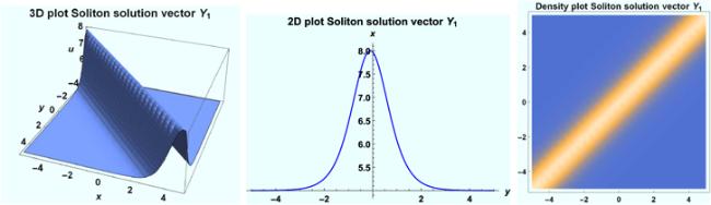
Figure 1. Bright soliton wave profile depicting solution ( |
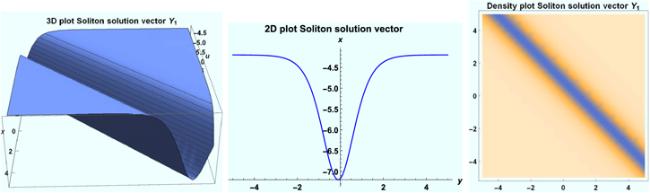
Figure 2. Dark soliton wave profile depicting solution ( |
Moreover, under vector Y2, the streaming behaviour of solution (3.27 ) is portrayed in figure 3 by letting $v=z\cos (y)-3/4\,{\rm{sech}} {\left(z\right)}^{2}\,\tanh (z)$, thus giving way for a periodic interaction between a kink and periodic solitons with different amplitudes. In addition, we delineate the dynamics of (3.28 ) via figure 4 with 3D, 2D alongside density plots using dissimilar parametric values c1 = 0.1, c2 = −0.01, c3 = 1, c4 = 1.2, c5 = 0.2 where variables −5.4 ≤ x, y ≤ 5.4, t = 0 and z = 0.4. We further represent the potency of soliton (3.31 ) via 3D plot, 2D plot as well as density plot in figure 5 with the values c1 = 0.1, c2 = −0.01, c3 = 1, c4 = 1.2, c5 = 0.2 where −5.4 ≤ x, y ≤ 5.4, t = 0 and z = 0.7. Now, we take ${F}_{1}(z/y)={cn}(z,y)$ in solution (3.36 ) thereby occasioning algebraic-periodic soliton interaction revealed in figure 6. Thus, this cause a spike in the region 0 ≤ x ≤ 2 with small wavelengths. We observe clearly that as x → −∞ the wave grows bigger and the reverse becomes the case as x → +∞. In water wave, energy of waves is compressed into a smaller volume as they reach the shore because water depth decreases thereby creating higher waves. This is called shoaling effect. In addition, a small wave or ripple that is observed on the surface of a liquid is refers to as a wavelet. Therefore, x → −∞ in figure 6 portrays shoaling effect of water wave while x → +∞ represent effects of wavelets on water. We generate solution (3.53 ) of (1.3 ) under vector Y5. Representing ${G}_{1}(z,t)={\rm{sech}} (t)+z\cos (t)$ in the solution, one observes an interaction between periodic alongside soliton solutions, which appear from variation in amplitude. This is revealed in figure 7.
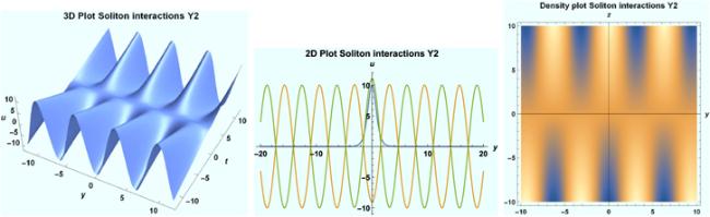
Figure 3. Soliton interactions wave profile for solution ( |
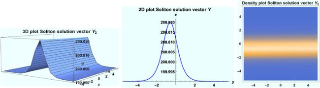
Figure 4. Bright soliton wave profile depicting solution ( |
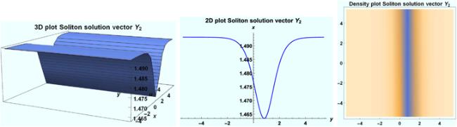
Figure 5. Dark soliton wave profile depicting solution ( |
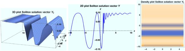
Figure 6. Soliton interaction wave depicting solution ( |
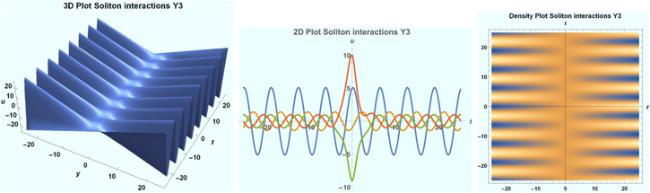
Figure 7. Soliton interactions wave profile depicting solution ( |
We show the dynamics of solution (3.47 ) via 3D plot, 2D plot as well as density plot in figure 8 by taking ${F}_{1}(z,t)=z\,{\rm{sech}} ({\rm{t}})+\tanh ({\rm{t}})$ thereby occasioning soliton interactions. Besides, figure 9 shows the streaming character of solution (3.50 ) in 3D, 2D alongside density plots by assuming ${F}_{1}(z,t)=z\,\mathrm{sn}(z,t)+{\rm{sech}} ({\rm{t}})$ which yields periodic soliton interactions at x = y = 0. In the same vein, logarithmic result (3.73 ) is depicted in figure 10 via 3D, 2D and density plots. This gives a soliton interactions with a spike at (z, y) = (0, 1) revealing a negligible wavelength, thereby possessing a small amplitude at the said point within the wave propagation. We achieve this by taking ${F}_{3}(z,t)={cn}(z,t)$ where we assign parametric values t = 10, x = 2, C1 = 10, C2 = 5.
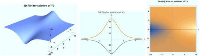
Figure 8. Soliton interactions wave profile depicting solution ( |
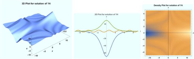
Figure 9. Soliton interactions wave profile depicting solution ( |

Figure 10. Soliton interactions wave profile depicting solution ( |
In addition, the figures are plotted in the interval −40 ≤ t, x ≤ 40 and y = 0 while z = 0. In figure 11, soliton solution (3.64 ) is plotted in the structure of 3D, 2D and density plots and the parameters are allocated values as C1 = 2, C2 = 0. Besides, t and x are in the interval −10 ≤ t, x ≤ 10 and y = z = 0. The demonstration of the dynamics of singular soliton solution (3.75 ) is given in figure 12 in form of 3D plot, 2D plot and density plot. In order to achieve that, the parameters in the solution are given dissimilar values as C1 = 1, C2 = 0.

Figure 11. Singular soliton wave profile of solution ( |

Figure 12. Singular soliton wave profile of solution ( |
Periodic exact travelling waves are pertinent with regards to the significant part they play in several physical problems. These problems include self-reinforcing systems, systems reaction-diffusion-advection impulsive systems, the list continues.
Now we contemplate the dark soliton wave solutions u1 and v1 given in (4.97 ). Figure 13 presents the graphic display of the streaming behaviour of (4.97 ) in 3D plot, 2D plot as well as density plot, where we allocate unalike values to the involved parameters as c = 0.1, θ1 = 3.1, θ2 = 0.000 001, ζ0 = 0, γ = −1.11, β0 = 1.029, a6 = −1, with y = z = 0, variables t and x are in the range −10 ≤ t, x ≤ 10. Figure 14 depicts the 3D, 2D and density plots of v1, where we have dissimilar values c = 0.0001, θ1 = 3.01, θ2 = 0.01, β0 = 2.187, ζ0 = 0, γ = −1.0001, a6 = 1, and y = z = 0, also variables t and x are in the range −10 ≤ t, x ≤ 10. It can be added here that figures 13 and 14 represent one-peak soliton wave profile of (4.97 ), see [64]. We sketch graphs of explosive/blowup solutions u2 and v2 expressed in (4.98 ). We observe that these solutions are singular anti-bell type soliton. Singular solitons solutions can be connected to a solitary wave whenever its centre becomes an imaginary position. Moreover, in clear terms, their intensity gets stronger, and as a result, they are not stable. It is discovered that these solutions have a cusp, which may eventually occasion the formation of rogue waves. The 3D plot, 2D plot and density plot of u2 is present in figure 15 with the varying values of the included parameters which are c = −0.000 02, θ1 = 1.1, θ2 = 1.002, β0 = 20.903 613, γ = −0.999 98, ζ0 = 0, a6 = 1, and y = z = 0, variables t and x are in the range −10 ≤ t, x ≤ 10. In order to view the streaming behaviour of solution v2, we presented the 3D plot, 2D plot together with density plot of v2 in figure 16 with different values of the parameters, that is, c = 0.002, θ1 = 1.6, θ2 = 1.2, β0 = 6.591, β1 = 1, β2 = 2, ζ0 = 0, γ = −1.002, C1 = 0, a6 = −1, and y = z = 0, whereas t and x are in the range −10 ≤ t, x ≤ 10. More so, we notice here the existence of a distinctive asymptotic structure observable for ${\mathrm{lim}}_{t\to 0}{v}_{2}(x,y,z,t)=-\infty $.

Figure 13. Anti-bell shape wave profile of soliton solution ( |

Figure 14. Anti-bell shape wave profile of soliton solution ( |

Figure 15. Singular anti-bell shape wave profile of soliton solution ( |

Figure 16. Singular anti-bell shape wave profile of soliton solution ( |
Furthermore, the dynamical behaviour of sinusoidal-type periodic soliton solutions u3 and v3 with singularities in (4.99 ) are exploited. In figure 17, the 3D, 2D and density plots of u3 are given with various values of the included parameters stated as c = 0.003, θ1 = 1.4, θ2 = 6.875, β0 = 3, γ = −1.003, ζ0 = 0, C1 = 0, a6 = 1 and y = z = 0, with −10 ≤ t, x ≤ 10. Figure 18 depicts the 3D plot, 2D plot and density plot of v3, where we assign the values c = 0.0002, θ1 = 1.3, θ2 = 5.6, β0 = 3, β1 = 0.5, β2 = 2, γ = −1.0002, ζ0 = 0, C1 = 0, a6 = −1, y = z = 0 and −10 ≤ t, x ≤ 10. We observe that the singularities of v3 exists in the time domain −10 ≤ t ≤ 10. Next we consider the singular soliton solutions u4 and v4 given respectively in (4.100a ) and (4.100b ) which are singular soliton solutions. We sketch the graphs of u4 in form of 3D, 2D and density plots in figure 19 with dissimilar values of included parameters which are c = 0.002, θ1 = 1.0005, β0 = 0.024, ζ0 = 0, γ = −1.002, a6 = −1, and y = z = 0, where t and x are within the interval −10 ≤ t, x ≤ 10. Figure 20 represents the streaming pattern of singular soliton solution v4 with unalike values of parameters c = 0.02, θ1 = 1.02, β0 = 3, β1 = −0.5, β2 = 2, C1 = 0, ζ0 = 0, γ = −1.02, a6 = 1, and y = z = 0. Variables t and x are in the domain −10 ≤ t, x ≤ 10. Accordingly, figures 19 and 8 depict singular bell shape soliton wave structure of solutions (4.100 ). Moreover, it is noteworthy to see that there is the existence of a distinctive asymptotic structure observable for ${\mathrm{lim}}_{t\to 0}{v}_{9}(x,y,z,t)=\infty $.

Figure 17. Singular periodic wave profile of soliton solution ( |

Figure 18. Singular periodic wave profile of soliton solution ( |

Figure 19. Bell-shaped singular soliton wave profile of ( |

Figure 20. Bell-shaped singular soliton wave profile of ( |
The dynamics of periodic soliton solution u5 and v5 presented in (4.105 ) and (4.106 ) are contemplated in figures 21 and 10 accordingly. The 3D plot, 2D plot together with density plot of u5 is plotted in figure 21 with varying values of parameters as c = 0.01, θ1 = 0.01, θ2 = 2.1, θ3 = 3.01, β0 = 5.184, γ = −1.01, ζ0 = 0, a6 = −1, and y = z = 0. Besides, variables t and x are in the intervals −10 ≤ t, x ≤ 10. In the actual sense, figure 21 exhibits a smooth periodic soliton wave profile of u5. Figure 22 shows the 3D, 2D as well as density plots of v5 where parameters c = 0.001, θ1 = 1.01, θ2 = 2.1, θ3 = 3.01, β0 = 2.187, β1 = 1, β2 = 2, C1 = 0, γ = −1.001, ζ0 = 0, a6 = 1, and variables y = z = 0. t and x are in the intervals −10 ≤ t, x ≤ 10. Appropriately, figure 22 displays a smooth periodic soliton wave structure of v5. We can put it that figures 21 and 22 respectively represent smooth multi-peak soliton wave of solutions u5 and v5.

Figure 21. Smooth periodic wave profile of soliton solution ( |

Figure 22. Smooth periodic wave profile of soliton solution ( |
We consider the streaming pattern of exact travelling wave solution u6 and v6 which are doubly-periodic soliton solutions expressed in (4.108 ) and (4.109 ) respectively. In figures 23, the 3D plot, 2D plot alongside density plot of u6 is demonstrated with dissimilar values of the engaged parameters such as c = 0.01, θ1 = 0.01, θ2 = 2.1, θ3 = 3.01, β0 = 3, γ = −1.01, ζ0 = 0, a6 = −1, with y = 0 and z = 0. Also, variables t and x are in the intervals −10 ≤ t, x ≤ 10. Solutions u6 and v6 have points of singularities and the singularities of u6 exist in the time domain −10 ≤ t ≤ 10. Figure 24 shows the 3D, 2D with density plots of v6 with unalike values of parameters c = 0.01, θ1 = 0.01, θ2 = 2.1, θ3 = 3.01, β0 = 1.842 375, ζ0 = 0, γ = −1.01, a6 = −1, where variables y = 0 and z = 0. In addition, t and x are in the intervals −10 ≤ t, x ≤ 10. We discover that singularities of v6 occur in the time domain −10 ≤ t ≤ 10.

Figure 23. Singular soliton wave profile of ( |

Figure 24. Singular soliton wave profile of ( |
Further, we contemplate the dynamical character of exact travelling wave solution u7 and v7. They are periodic soliton solutions given in (4.112 ) and (4.113 ) respectively. We demonstrate that for u7 with 3D plot, 2D plot as well as density plot in figure 25. The dissimilar values of the included parameters are given as c = 0.01, θ1 = 0.01, θ2 = 2.1, θ3 = 1.01, β0 = 1.536, γ = −1.01, ζ0 = 0, b = 0.1, e = 2.01, a6 = −1, such that y = 0 and z = 0. Besides, variables t and x are in the intervals −10 ≤ t, x ≤ 10. Thus, figure 25 depicts a smooth periodic soliton wave profile of u7. Lastly, figure 26 reveals the streaming pattern of v7 in the form of 3D, 2D and density plots. The varying values of the involved parameters are stated as c = 0.001, θ1 = 0.01, θ2 = 0.1, θ3 = 1.01, β0 = 1.842 375, β1 = 1, β2 = 1, C1 = 0.01, b = 0.01, e = 2.01, γ = −1.001, ζ0 = 0, a6 = −1, where variables y = 0 and z = 0, t and x are also in the intervals −10 ≤ t, x ≤ 10. Therefore, figure 26 exhibits the smooth periodic soliton wave profile of v7. We can conclude that figures 25 and 26 represent smooth multi-peak soliton wave of solutions (4.112 ) and (4.113 ) respectively.

Figure 25. Periodic soliton wave profile of soliton solution ( |

Figure 26. Periodic soliton wave profile of soliton solution ( |
6. Conclusions
This paper presented the study carried out on the three-dimensional soliton equation (1.3 ). Diverse new exact travelling wave and soliton solutions were secured for the equation under consideration with the implementation of Lie group theory. The solutions constructed comprises the solitary wave solutions, elliptic wave solutions, soliton wave solutions, periodic (hyperbolic) wave as well as rational solutions functions. The advantage which such functions have is that they enable us to conveniently comment on the physical behaviour of the wave, notwithstanding the range of the graphs possessed by the resulting solution function. Hyperbolic functions and trigonometric functions are emergent in both physics and mathematics. For instance, hyperbolic cosine functions are found out to possess the shape of a catenary. Moreover, the hyperbolic tangent functions appear in the calculation of magnetic moment together with the rapidity of special relativity, which by extension, applies in quantum physics. In addition, hyperbolic secant functions emerge in the profile of a laminar jet. We also have it that hyperbolic cotangent functions come to light in the Langevin function for magnetic polarization [65]. Langevin function is a special function that appears when studying an idealized paramagnetic material in statistical mechanics. Using the method of polynomial complete discriminant system and elementary integral, we achieved various solitonic solutions which are new solutions obtained for the model under study. The results secured here revealed that the technique engaged in this study can better solve nonlinear differential equations to achieve the solutions that are not available when other methods are put to use. In addition, we took special cases of some functions in the obtained symmetries and performed symmetry reduction of the underlying equation thereby furnishing logarithmic results among others. Moreover, in a bid to have a distinct and clear understanding of the physical properties of the reported closed-form solutions, a suitable choice of values of parameters was made to plot 3D, 2D and the density graphs of the solutions. Lastly, we constructed the conserved vectors of (1.3 ) by utilizing the standard multiplier technique via homotopy formula. The achieved solutions in this paper could be of importance to explain some practical physical problems that arise in physics, engineering and other nonlinear sciences.
Appendix. Prolongation coefficients: full expansions
$\begin{eqnarray*}\begin{array}{l}{\left({\phi }^{1}\right)}^{t}={\phi }_{t}^{1}+{u}_{t}{\phi }_{u}^{1}+{v}_{t}{\phi }_{v}^{1}-{u}_{t}{\xi }_{t}^{4}\\ -\ {u}_{t}^{2}{\xi }_{u}^{4}-{u}_{t}{v}_{t}{\xi }_{v}^{4}-{u}_{x}{\xi }_{t}^{1}-{u}_{x}{u}_{t}{\xi }_{u}^{1}\\ -\ {u}_{x}{v}_{t}{\xi }_{v}^{1}-{u}_{y}{\xi }_{t}^{2}-{u}_{y}{u}_{t}{\xi }_{u}^{2}-{u}_{y}{v}_{t}{\xi }_{v}^{2}\\ -\ {u}_{z}{\xi }_{t}^{3}-{u}_{t}{u}_{z}{\xi }_{u}^{3}-{u}_{z}{v}_{t}{\xi }_{v}^{3},\end{array}\end{eqnarray*}$
$\begin{eqnarray*}\begin{array}{l}{\left({\phi }^{1}\right)}^{x}={\phi }_{x}^{1}+{u}_{x}{\phi }_{u}^{1}+{v}_{x}{\phi }_{v}^{1}\\ -\ {u}_{t}{\xi }_{x}^{4}-{u}_{t}{u}_{x}{\xi }_{u}^{4}-{u}_{t}{v}_{x}{\xi }_{v}^{4}-{u}_{x}{\xi }_{x}^{1}\\ -\ {u}_{x}^{2}{\xi }_{u}^{1}-{u}_{x}{v}_{x}{\xi }_{v}^{1}-{u}_{y}{\xi }_{x}^{2}-{u}_{y}{u}_{x}{\xi }_{u}^{2}\\ -\ {u}_{y}{v}_{x}{\xi }_{v}^{2}-{u}_{z}{\xi }_{x}^{3}-{u}_{z}{u}_{x}{\xi }_{u}^{3}-{u}_{z}{v}_{x}{\xi }_{v}^{3},\end{array}\end{eqnarray*}$
$\begin{eqnarray*}\begin{array}{l}{\left({\phi }^{2}\right)}^{x}={\phi }_{x}^{2}+{u}_{x}{\phi }_{u}^{2}+{v}_{x}{\phi }_{v}^{2}\\ -\ {v}_{t}{\xi }_{x}^{4}-{v}_{t}{u}_{x}{\xi }_{u}^{4}-{v}_{t}{v}_{x}{\xi }_{v}^{4}-{v}_{x}{\xi }_{x}^{1}\\ -\ {u}_{x}{v}_{x}{\xi }_{u}^{1}-{v}_{x}^{2}{\xi }_{v}^{1}-{v}_{y}{\xi }_{x}^{2}\\ -\ {u}_{x}{v}_{y}{\xi }_{u}^{2}-{v}_{x}{v}_{y}{\xi }_{v}^{2}-{v}_{z}{\xi }_{x}^{3}\\ -\ {u}_{x}{v}_{z}{\xi }_{u}^{3}-{v}_{x}{v}_{z}{\xi }_{v}^{3},\end{array}\end{eqnarray*}$
$\begin{eqnarray*}\begin{array}{l}{\left({\phi }^{1}\right)}^{y}={\phi }_{y}^{1}+{u}_{y}{\phi }_{u}^{1}+{v}_{y}{\phi }_{v}^{1}\\ -\ {u}_{t}{\xi }_{y}^{4}-{u}_{t}{u}_{y}{\xi }_{u}^{4}-{u}_{t}{v}_{y}{\xi }_{v}^{4}\\ -\ {u}_{x}{\xi }_{y}^{1}-{u}_{x}{u}_{y}{\xi }_{u}^{1}-{u}_{x}{v}_{y}{\xi }_{v}^{1}\\ -\ {u}_{y}{\xi }_{y}^{2}-{u}_{y}^{2}{\xi }_{u}^{2}-{u}_{{{yv}}_{y}}{\xi }_{v}^{2}\\ -\ {u}_{z}{\xi }_{y}^{3}-{u}_{y}{u}_{z}{\xi }_{u}^{3}-{v}_{y}{u}_{z}{\xi }_{v}^{3},\end{array}\end{eqnarray*}$
$\begin{eqnarray*}\begin{array}{l}{\left({\phi }^{1}\right)}^{z}={\phi }_{z}^{1}+{u}_{z}{\phi }_{u}^{1}+{v}_{z}{\phi }_{v}^{1}\\ -\ {u}_{t}{\xi }_{z}^{4}-{u}_{t}{u}_{z}{\xi }_{u}^{4}-{u}_{t}{v}_{z}{\xi }_{v}^{4}\\ -\ {u}_{x}{\xi }_{z}^{1}-{u}_{x}{u}_{z}{\xi }_{u}^{1}-{u}_{x}{v}_{z}{\xi }_{v}^{1}\\ -\ {u}_{y}{\xi }_{z}^{2}-{u}_{y}{u}_{z}{\xi }_{u}^{2}-{u}_{y}{v}_{z}{\xi }_{v}^{2}\\ -\ {u}_{z}{\xi }_{z}^{3}-{u}_{z}^{2}{\xi }_{u}^{3}-{u}_{z}{v}_{z}{\xi }_{v}^{3},\end{array}\end{eqnarray*}$
$\begin{eqnarray*}\begin{array}{l}{\left({\phi }^{1}\right)}^{{yt}}=-{u}_{x}{u}_{t}{\xi }_{{yu}}^{1}-{u}_{t}{u}_{y}{\xi }_{{tu}}^{4}\\ -\ {u}_{x}{v}_{{ty}}{\xi }_{v}^{1}-{u}_{{ty}}{v}_{t}{\xi }_{v}^{4}+{u}_{y}{\phi }_{{tu}}^{1}\\ -\ {u}_{t}^{2}{\xi }_{{yu}}^{4}-{u}_{t}{\xi }_{{yt}}^{4}\\ -\ {u}_{{ty}}{v}_{y}{\xi }_{v}^{2}-{u}_{t}{v}_{y}{\xi }_{{tv}}^{4}-{u}_{y}{u}_{t}{\xi }_{{yu}}^{2}\\ -\ {u}_{z}{u}_{y}{u}_{t}{\xi }_{{uu}}^{3}-{u}_{x}{u}_{y}{u}_{t}{\xi }_{{uu}}^{1}\\ -\ {u}_{z}{u}_{t}{v}_{y}{\xi }_{{uv}}^{3}-{u}_{t}{u}_{{yz}}{\xi }_{u}^{3}\\ -\ {u}_{z}{u}_{t}{\xi }_{{yu}}^{3}-{u}_{x}{v}_{t}{\xi }_{{yv}}^{1}-{u}_{y}{u}_{z}{v}_{t}{\xi }_{{uv}}^{3}\\ -\ {u}_{z}{v}_{t}{v}_{y}{\xi }_{{vv}}^{3}-{u}_{t}{v}_{t}{v}_{y}{\xi }_{{vv}}^{4}\\ -\ {u}_{x}{v}_{t}{v}_{y}{\xi }_{{vv}}^{1}-{u}_{y}^{2}{v}_{t}{\xi }_{{uv}}^{2}-{u}_{{yz}}{v}_{t}{\xi }_{v}^{3}\\ -\ {u}_{{xy}}{v}_{t}{\xi }_{v}^{1}-{u}_{t}{v}_{{ty}}{\xi }_{v}^{4}-{u}_{z}{v}_{y}{\xi }_{{tv}}^{3}\\ -\ {u}_{x}{u}_{{ty}}{\xi }_{u}^{1}-{u}_{{yy}}{u}_{t}{\xi }_{u}^{2}-{u}_{{xy}}{u}_{t}{\xi }_{u}^{1}\\ -\ {u}_{t}{u}_{y}{v}_{t}{\xi }_{{uv}}^{4}-{u}_{t}{v}_{t}{\xi }_{{yv}}^{4}-{u}_{{tt}}{u}_{y}{\xi }_{u}^{4}\\ +\ {u}_{t}{v}_{y}{\phi }_{{uv}}^{1}-{u}_{z}{u}_{{ty}}{\xi }_{u}^{3}-{u}_{t}^{2}{v}_{y}{\xi }_{{uv}}^{4}\\ +\ {u}_{t}{\phi }_{{yu}}^{1}-{u}_{y}{v}_{y}{v}_{t}{\xi }_{{vv}}^{2}-{u}_{y}{v}_{y}{u}_{t}{\xi }_{{uv}}^{2}\\ -\ {u}_{x}{u}_{t}{v}_{y}{\xi }_{{uv}}^{1}-{u}_{x}{u}_{y}{v}_{t}{\xi }_{{uv}}^{1}-{u}_{z}{v}_{{ty}}{\xi }_{v}^{3}\\ -\ 2{u}_{t}{u}_{{ty}}{\xi }_{u}^{4}-{u}_{y}{v}_{{ty}}{\xi }_{v}^{2}+{\phi }_{{yt}}^{1}\\ -\ {u}_{z}{\xi }_{{yt}}^{3}+{u}_{{ty}}{\phi }_{u}^{1}-{u}_{{yy}}{\xi }_{t}^{2}-{u}_{{xy}}{\xi }_{t}^{1}\\ -\ {u}_{{yz}}{\xi }_{t}^{3}-{u}_{{tz}}{\xi }_{y}^{3}-{u}_{{ty}}{\xi }_{y}^{2}-{u}_{{tx}}{\xi }_{y}^{1}\\ -\ {u}_{{tt}}{\xi }_{y}^{4}-{u}_{y}{\xi }_{{yt}}^{2}-{u}_{z}{u}_{y}{\xi }_{{tu}}^{3}\\ -\ {u}_{y}{v}_{t}{\xi }_{{yv}}^{2}-{u}_{y}{u}_{t}^{2}{\xi }_{{uu}}^{4}\\ -\ {u}_{x}{v}_{y}{\xi }_{{tv}}^{1}-{u}_{{yy}}{v}_{t}{\xi }_{v}^{2}\\ -\ {u}_{y}^{2}{\xi }_{{tu}}^{2}-{u}_{x}{\xi }_{{yt}}^{1}-{u}_{z}{v}_{t}{\xi }_{{yv}}^{3}\\ +\ {v}_{y}{v}_{t}{\phi }_{{vv}}^{1}-{u}_{y}{u}_{{tz}}{\xi }_{u}^{3}-{u}_{x}{u}_{y}{\xi }_{{ut}}^{1}\\ -{u}_{{tt}}{v}_{y}{\xi }_{v}^{4}+{u}_{y}{v}_{t}{\phi }_{{uv}}^{1}-{u}_{{tx}}{u}_{y}{\xi }_{u}^{1}\\ +\ {u}_{y}{u}_{t}{\phi }_{{uu}}^{1}-2\,{u}_{y}{u}_{{ty}}{\xi }_{u}^{2}+{v}_{t}{\phi }_{{yv}}^{1}\\ +\ {v}_{{ty}}{\phi }_{v}^{1}+{v}_{y}{\phi }_{{tv}}^{1}-{u}_{{ty}}{\xi }_{t}^{4}-{u}_{{tz}}{v}_{y}{\xi }_{v}^{3}\\ -\ {u}_{{tx}}{v}_{y}{\xi }_{v}^{1}-{u}_{y}{v}_{y}{\xi }_{{tv}}^{2}-{u}_{y}^{2}{u}_{t}{\xi }_{{uu}}^{2},\end{array}\end{eqnarray*}$
$\begin{eqnarray*}\begin{array}{l}{\left({\phi }^{1}\right)}^{{xx}}=2\,{v}_{x}{u}_{x}{\phi }_{{uv}}^{1}-2\,{u}_{x}^{2}{v}_{x}{\xi }_{{uv}}^{1}\\ -\ 2\,{u}_{x}{u}_{{xy}}{\xi }_{u}^{2}-2\,{u}_{y}{v}_{x}{\xi }_{{xv}}^{2}-2\,{u}_{{xz}}{v}_{x}{\xi }_{v}^{3}\\ -\ 2\,{u}_{{tx}}{v}_{x}{\xi }_{v}^{4}-2\,{u}_{z}{u}_{x}{\xi }_{{ux}}^{3}-2\,{u}_{{xx}}{v}_{x}{\xi }_{v}^{1}\\ -\ 2\,{u}_{{xy}}{v}_{x}{\xi }_{v}^{2}-2\,{u}_{z}{v}_{x}{\xi }_{{xv}}^{3}-2\,{u}_{t}{v}_{x}{\xi }_{{xv}}^{4}\\ -\ 2\,{u}_{x}{v}_{x}{\xi }_{{xv}}^{1}-2\,{u}_{t}{u}_{x}{\xi }_{{xu}}^{4}-2\,{u}_{y}{u}_{x}{\xi }_{{xu}}^{2}\\ -\ 2\,{u}_{x}{u}_{{xz}}{\xi }_{u}^{3}-2\,{u}_{x}{u}_{{tx}}{\xi }_{u}^{4}-3\,{u}_{x}{u}_{{xx}}{\xi }_{u}^{1}\\ +{\phi }_{{xx}}^{1}+{u}_{{xx}}{\phi }_{u}^{1}-{u}_{y}{\xi }_{{xx}}^{2}-{u}_{x}{\xi }_{{xx}}^{1}\\ -\ {u}_{z}{\xi }_{{xx}}^{3}-{u}_{x}^{3}{\xi }_{{uu}}^{1}-{u}_{t}{\xi }_{{xx}}^{4}\\ +\ {u}_{x}^{2}{\phi }_{{uu}}^{1}+{v}_{{xx}}{\phi }_{v}^{1}+{v}_{x}^{2}{\phi }_{{vv}}^{1}\\ -2\,{u}_{x}^{2}{\xi }_{{xu}}^{1}+2\,{u}_{x}{\phi }_{{xu}}^{1}+2\,{v}_{x}{\phi }_{{xv}}^{1}\\ -\ 2\,{u}_{{xz}}{\xi }_{x}^{3}-2\,{u}_{{xx}}{\xi }_{x}^{1}-2\,{u}_{{xy}}{\xi }_{x}^{2}\\ -\ 2\,{u}_{{tx}}{\xi }_{x}^{4}-{u}_{t}{u}_{{xx}}{\xi }_{u}^{4}-2\,{u}_{z}{u}_{x}{v}_{x}{\xi }_{{vu}}^{3}\\ -\ 2\,{u}_{t}{u}_{x}{v}_{x}{\xi }_{{vu}}^{4}-2\,{u}_{y}{u}_{x}{v}_{x}{\xi }_{{vu}}^{2}\\ -\ {u}_{{xx}}{u}_{y}{\xi }_{u}^{2}-{u}_{z}{v}_{{xx}}{\xi }_{v}^{3}-{u}_{t}{v}_{{xx}}{\xi }_{v}^{4}\\ -\ {u}_{x}{v}_{{xx}}{\xi }_{v}^{1}-{u}_{y}{v}_{{xx}}{\xi }_{v}^{2}-{u}_{x}{v}_{x}^{2}{\xi }_{{vv}}^{1}\\ -\ {u}_{y}{v}_{x}^{2}{\xi }_{{vv}}^{2}-{u}_{z}{v}_{x}^{2}{\xi }_{{vv}}^{3}-{u}_{t}{v}_{x}^{2}{\xi }_{{vv}}^{4}\\ -\ {u}_{z}{u}_{x}^{2}{\xi }_{{uu}}^{3}-{u}_{t}{u}_{x}^{2}{\xi }_{{uu}}^{4}-{u}_{y}{u}_{x}^{2}{\xi }_{{uu}}^{2}\\ -\ {u}_{{xx}}{u}_{z}{\xi }_{u}^{3},\end{array}\end{eqnarray*}$
$\begin{eqnarray*}\begin{array}{l}{\left({\phi }^{2}\right)}^{{xx}}={\phi }_{{xx}}^{2}-2\,{v}_{t}{u}_{x}{v}_{x}{\xi }_{{uv}}^{4}\\ -\ 2\,{v}_{y}{u}_{x}{v}_{x}{\xi }_{{uv}}^{2}-2\,{v}_{x}{v}_{z}{u}_{x}{\xi }_{{uv}}^{3}\\ -\ 2\,{u}_{x}{v}_{x}{\xi }_{{ux}}^{1}-2\,{u}_{x}{v}_{x}^{2}{\xi }_{{uv}}^{1}\\ -\ 2\,{u}_{x}{v}_{y}{\xi }_{{ux}}^{2}-2\,{v}_{x}{v}_{y}{\xi }_{{xv}}^{2}\\ -\ 2\,{v}_{t}{u}_{x}{\xi }_{{ux}}^{4}-2\,{v}_{t}{v}_{x}{\xi }_{{xv}}^{4}\\ -\ 2\,{u}_{x}{v}_{z}{\xi }_{{ux}}^{3}-2\,{v}_{x}{v}_{z}{\xi }_{{xv}}^{3}\\ +\ 2\,{u}_{x}{v}_{x}{\phi }_{{uv}}^{2}-2\,{u}_{x}{v}_{{tx}}{\xi }_{u}^{4}\\ -\ 2\,{v}_{{tx}}{v}_{x}{\xi }_{v}^{4}-2\,{u}_{x}{v}_{{xx}}{\xi }_{u}^{1}\\ -\ 3\,{v}_{x}{v}_{{xx}}{\xi }_{v}^{1}-2\,{u}_{x}{v}_{{xy}}{\xi }_{u}^{2}\\ -\ 2\,{v}_{x}{v}_{{xy}}{\xi }_{v}^{2}-2\,{u}_{x}{v}_{{xz}}{\xi }_{u}^{3}\\ -\ 2\,{v}_{x}{v}_{{xz}}{\xi }_{v}^{3}-{u}_{{xx}}{v}_{t}{\xi }_{u}^{4}\\ -\ {v}_{x}{u}_{{xx}}{\xi }_{u}^{1}-{u}_{{xx}}{v}_{y}{\xi }_{u}^{2}\\ -\ {v}_{z}{\xi }_{u}^{3}{u}_{{xx}}-{v}_{t}{u}_{x}^{2}{\xi }_{{uu}}^{4}-{v}_{t}{v}_{x}^{2}{\xi }_{{vv}}^{4}\\ -\ {v}_{x}{u}_{x}^{2}{\xi }_{{uu}}^{1}-{v}_{y}{u}_{x}^{2}{\xi }_{{uu}}^{2}-{v}_{y}{v}_{x}^{2}{\xi }_{{vv}}^{2}\\ -\ {v}_{z}{u}_{x}^{2}{\xi }_{{uu}}^{3}-{v}_{z}{v}_{x}^{2}{\xi }_{{vv}}^{3}-{v}_{t}{v}_{{xx}}{\xi }_{v}^{4}\\ -\ {v}_{y}{v}_{{xx}}{\xi }_{v}^{2}-{v}_{{xx}}{v}_{z}{\xi }_{v}^{3}-{v}_{t}{\xi }_{{xx}}^{4}\\ +\ {v}_{{xx}}{\phi }_{v}^{2}-\ {v}_{x}{\xi }_{{xx}}^{1}-{v}_{x}^{3}{\xi }_{{vv}}^{1}-{v}_{y}{\xi }_{{xx}}^{2}-{v}_{z}{\xi }_{{xx}}^{3}\\ +\ {v}_{x}^{2}{\phi }_{{vv}}^{2}+{u}_{{xx}}{\phi }_{u}^{2}+{u}_{x}^{2}{\phi }_{{uu}}^{2}\\ -\ 2\,{v}_{{xx}}{\xi }_{x}^{1}-2\,{v}_{{xy}}{\xi }_{x}^{2}-2\,{v}_{{xz}}{\xi }_{x}^{3}\\ -2\,{v}_{{tx}}{\xi }_{x}^{4}+2\,{v}_{x}{\phi }_{{xv}}^{2}-2\,{v}_{x}^{2}{\xi }_{{xv}}^{1}\\ +\ 2\,{u}_{x}{\phi }_{{xu}}^{2},\end{array}\end{eqnarray*}$
$\begin{eqnarray*}\begin{array}{l}{\left({\phi }^{1}\right)}^{{xy}}={\phi }_{x}^{1}-{u}_{z}{u}_{x}{v}_{y}{\xi }_{{uv}}^{3}\\ -\ {u}_{y}{u}_{z}{v}_{x}{\xi }_{{uv}}^{3}-{u}_{z}{v}_{x}{v}_{y}{\xi }_{{vv}}^{3}\\ -\ {u}_{x}{u}_{y}{v}_{x}{\xi }_{{uv}}^{1}-{u}_{x}{v}_{x}{v}_{y}{\xi }_{{vv}}^{1}\\ -\ {u}_{y}{u}_{x}{v}_{y}{\xi }_{{uv}}^{2}-{u}_{y}{v}_{x}{v}_{y}{\xi }_{{vv}}^{2}\\ +\ {u}_{y}{v}_{x}{\phi }_{{uv}}^{1}+{v}_{x}{v}_{y}{\phi }_{{vv}}^{1}-{u}_{t}{v}_{y}{\xi }_{{xv}}^{4}\\ -\ {u}_{x}{v}_{y}{\xi }_{{xv}}^{1}-{u}_{x}^{2}{v}_{y}{\xi }_{{uv}}^{1}\\ +\ {u}_{x}{v}_{y}{\phi }_{{uv}}^{1}-{u}_{y}{v}_{y}{\xi }_{{xv}}^{2}-{u}_{z}{v}_{y}{\xi }_{{xv}}^{3}\\ -\ {u}_{{tx}}{v}_{y}{\xi }_{v}^{4}-{u}_{{xx}}{v}_{y}{\xi }_{v}^{1}-{u}_{{xy}}{v}_{y}{\xi }_{v}^{2}\\ -\ {u}_{{xz}}{v}_{y}{\xi }_{v}^{3}-{u}_{{ty}}{v}_{x}{\xi }_{v}^{4}-{u}_{{xy}}{v}_{x}{\xi }_{v}^{1}\\ -\ {u}_{{yy}}{v}_{x}{\xi }_{v}^{2}-{u}_{{yz}}{v}_{x}{\xi }_{v}^{3}-{u}_{x}{v}_{x}{\xi }_{{vy}}^{1}\\ -\ {u}_{t}{v}_{{xy}}{\xi }_{v}^{4}-{u}_{x}{v}_{{xy}}{\xi }_{v}^{1}-{u}_{y}{v}_{{xy}}{\xi }_{v}^{2}\\ -\ {u}_{z}{v}_{{xy}}{\xi }_{v}^{3}-{u}_{t}{u}_{x}{u}_{y}{\xi }_{{uu}}^{4}\\ -\ {u}_{t}{v}_{x}{\xi }_{{vy}}^{4}-{u}_{z}{u}_{x}{u}_{y}{\xi }_{{uu}}^{3}\\ -\ {u}_{t}{u}_{x}{v}_{y}{\xi }_{{vu}}^{4}-{u}_{t}{u}_{y}{v}_{x}{\xi }_{{vu}}^{4}\\ -\ {u}_{t}{v}_{x}{v}_{y}{\xi }_{{vv}}^{4}-{u}_{y}{u}_{z}{\xi }_{{xu}}^{3}\\ -\ {u}_{{tx}}{u}_{y}{\xi }_{u}^{4}-{u}_{{xx}}{u}_{y}{\xi }_{u}^{1}-{u}_{{xz}}{u}_{y}{\xi }_{u}^{3}\\ -\ {u}_{x}{u}_{{ty}}{\xi }_{u}^{4}-{u}_{t}{u}_{{xy}}{\xi }_{u}^{4}\\ -\ {u}_{x}{u}_{{yy}}{\xi }_{u}^{2}-{u}_{{yz}}{u}_{x}{\xi }_{u}^{3}\\ -\ {u}_{z}{u}_{{xy}}{\xi }_{u}^{3}-{u}_{t}{u}_{x}{\xi }_{{uy}}^{4}-{u}_{y}{u}_{x}{\xi }_{{uy}}^{2}\\ -\ {u}_{y}^{2}{u}_{x}{\xi }_{{uu}}^{2}-{u}_{z}{u}_{x}{\xi }_{{uy}}^{3}-{u}_{t}{u}_{y}{\xi }_{{ux}}^{4}\\ -\ {u}_{{yy}}{\xi }_{x}^{2}-{u}_{x}^{2}{u}_{y}{\xi }_{{uu}}^{1}+{u}_{x}{u}_{y}{\phi }_{{uu}}^{1}\\ -\ {u}_{y}{v}_{x}{\xi }_{{vy}}^{2}-{u}_{y}^{2}{v}_{x}{\xi }_{{vu}}^{2}-{u}_{z}{v}_{x}{\xi }_{{vy}}^{3}\\ +\ {\phi }_{v}^{1}{v}_{{xy}}+{v}_{x}{\phi }_{{vy}}^{1}-{u}_{t}{\xi }_{{xy}}^{4}+{v}_{y}{\phi }_{{vx}}^{1}\\ -\ {u}_{x}{\xi }_{{xy}}^{1}-{u}_{x}^{2}{\xi }_{{uy}}^{1}+{u}_{x}{\phi }_{{uy}}^{1}-{u}_{y}{\xi }_{{xy}}^{2}\\ -\ {u}_{y}^{2}{\xi }_{{xu}}^{2}-{u}_{z}{\xi }_{{xy}}^{3}+{u}_{y}{\phi }_{{xu}}^{1}\\ -\ {u}_{{tx}}{\xi }_{y}^{4}-{u}_{{xx}}{\xi }_{y}^{1}-{u}_{{xy}}{\xi }_{y}^{2}\\ -\ {u}_{{xz}}{\xi }_{y}^{3}-{u}_{{ty}}{\xi }_{x}^{4}-{u}_{{xy}}{\xi }_{x}^{1}\\ +\ {u}_{{xy}}{\phi }_{u}^{1}-{u}_{x}{u}_{y}{\xi }_{{ux}}^{1}-{u}_{{yz}}{\xi }_{x}^{3}\\ -\ 2\,{u}_{x}{u}_{{xy}}{\xi }_{u}^{1}-2\,{u}_{y}{u}_{{xy}}{\xi }_{u}^{2},\end{array}\end{eqnarray*}$
$\begin{eqnarray*}\begin{array}{l}{\left({\phi }^{1}\right)}^{{xz}}={v}_{{xz}}{\phi }_{v}^{1}-{u}_{z}{v}_{{xz}}{\xi }_{v}^{3}\\ -\ {u}_{t}{v}_{{xz}}{\xi }_{v}^{4}-{u}_{x}{v}_{{xz}}{\xi }_{v}^{1}\\ -\ {u}_{z}{v}_{x}{\xi }_{{vz}}^{3}-{u}_{z}^{2}{v}_{x}{\xi }_{{vu}}^{3}-{u}_{t}{v}_{x}{\xi }_{{vz}}^{4}\\ -\ {u}_{x}{v}_{x}{\xi }_{{vz}}^{1}-{u}_{y}{v}_{x}{\xi }_{{vz}}^{2}-{u}_{x}{u}_{{zz}}{\xi }_{u}^{3}\\ -\ {u}_{x}{u}_{{tz}}{\xi }_{u}^{4}-{u}_{t}{u}_{{xz}}{\xi }_{u}^{4}-{u}_{x}{u}_{{yz}}{\xi }_{u}^{2}\\ -\ {u}_{y}{u}_{{xz}}{\xi }_{u}^{2}-{u}_{{xx}}{u}_{z}{\xi }_{u}^{1}-{u}_{{xy}}{u}_{z}{\xi }_{u}^{2}\\ -\ {u}_{{tx}}{u}_{z}{\xi }_{u}^{4}-{u}_{y}{v}_{z}{\xi }_{{xv}}^{2}-{u}_{z}{v}_{z}{\xi }_{{xv}}^{3}\\ +\ {u}_{x}{v}_{z}{\phi }_{{uv}}^{1}+{u}_{z}{v}_{x}{\phi }_{{uv}}^{1}+{v}_{x}{v}_{z}{\phi }_{{vv}}^{1}\\ -\ {u}_{t}{v}_{z}{\xi }_{{xv}}^{4}-{u}_{x}{v}_{z}{\xi }_{{xv}}^{1}-{u}_{x}^{2}{v}_{z}{\xi }_{{uv}}^{1}\\ -\ {u}_{{zz}}{v}_{x}{\xi }_{v}^{3}-{u}_{{tz}}{v}_{x}{\xi }_{v}^{4}-{u}_{z}{u}_{x}{\xi }_{{zu}}^{3}\\ -\ {u}_{z}^{2}{u}_{x}{\xi }_{{uu}}^{3}-{u}_{t}{u}_{x}{\xi }_{{zu}}^{4}-{u}_{y}{u}_{x}{\xi }_{{zu}}^{2}\\ -\ {u}_{y}{u}_{z}{\xi }_{{xu}}^{2}+{u}_{x}{u}_{z}{\phi }_{{uu}}^{1}-{u}_{t}{u}_{z}{\xi }_{{xu}}^{4}\\ -\ {u}_{x}{u}_{z}{\xi }_{{xu}}^{1}-{u}_{x}^{2}{u}_{z}{\xi }_{{uu}}^{1}-{u}_{y}{v}_{{xz}}{\xi }_{v}^{2}\\ +\ {\phi }_{{xz}}^{1}-2\,{u}_{z}{u}_{{xz}}{\xi }_{u}^{3}-2\,{u}_{x}{u}_{{xz}}{\xi }_{u}^{1}\\ -\ {u}_{{xz}}{v}_{x}{\xi }_{v}^{1}-{u}_{{yz}}{v}_{x}{\xi }_{v}^{2}-{u}_{{xx}}{v}_{z}{\xi }_{v}^{1}\\ -\ {u}_{{xy}}{v}_{z}{\xi }_{v}^{2}-{u}_{{xz}}{v}_{z}{\xi }_{v}^{3}-{u}_{{tx}}{v}_{z}{\xi }_{v}^{4}\\ -\ {u}_{t}{u}_{x}{u}_{z}{\xi }_{{uu}}^{4}-{u}_{y}{u}_{x}{u}_{z}{\xi }_{{uu}}^{2}\\ -\ {u}_{z}{u}_{x}{v}_{z}{\xi }_{{uv}}^{3}-{u}_{z}{v}_{x}{v}_{z}{\xi }_{{vv}}^{3}\\ -\ {u}_{t}{u}_{x}{v}_{z}{\xi }_{{uv}}^{4}-{u}_{t}{v}_{x}{u}_{z}{\xi }_{{uv}}^{4}\\ -\ {u}_{t}{v}_{x}{v}_{z}{\xi }_{{vv}}^{4}-{u}_{x}{u}_{z}{v}_{x}{\xi }_{{uv}}^{1}\\ -\ {u}_{x}{v}_{x}{v}_{z}{\xi }_{{vv}}^{1}-{u}_{y}{u}_{x}{v}_{z}{\xi }_{{uv}}^{2}\\ -\ {u}_{y}{u}_{z}{v}_{x}{\xi }_{{uv}}^{2}-{u}_{y}{v}_{x}{v}_{z}{\xi }_{{vv}}^{2}\\ -\ {u}_{t}{\xi }_{{xz}}^{4}-{u}_{x}{\xi }_{{xz}}^{1}-{u}_{x}^{2}{\xi }_{{zu}}^{1}\\ -\ {u}_{y}{\xi }_{{xz}}^{2}-{u}_{z}{\xi }_{{xz}}^{3}-{u}_{z}^{2}{\xi }_{{xu}}^{3}\\ +\ {u}_{x}{\phi }_{{zu}}^{1}+{u}_{z}{\phi }_{{xu}}^{1}-{u}_{{xx}}{\xi }_{z}^{1}-{u}_{{xy}}{\xi }_{z}^{2}\\ -\ {u}_{{xz}}{\xi }_{z}^{3}-{u}_{{tx}}{\xi }_{z}^{4}-{u}_{{yz}}{\xi }_{x}^{2}-{u}_{{zz}}{\xi }_{x}^{3}\\ +\ {u}_{{xz}}{\phi }_{u}^{1}-{u}_{{tz}}{\xi }_{x}^{4}-{u}_{{xz}}{\xi }_{x}^{1}+{v}_{x}{\phi }_{{vz}}^{1}\\ +\ {v}_{z}{\phi }_{{vx}}^{1},\end{array}\end{eqnarray*}$
$\begin{eqnarray*}\begin{array}{l}{\left({\phi }^{1}\right)}^{{xxxy}}={\phi }_{{xxxy}}^{1}-3\,{u}_{{xxyy}}{\xi }_{x}^{2}\\ +\ 3\,{u}_{{xxy}}{\phi }_{{xu}}^{1}+3\,{u}_{{xx}}{\phi }_{{xyu}}^{1}+{u}_{{xxx}}{\phi }_{{uy}}^{1}\\ -\ 3\,{u}_{{xxx}}{\xi }_{{xy}}^{1}-3\,{u}_{{txx}}{\xi }_{{xy}}^{4}-{u}_{{xxxz}}{\xi }_{y}^{3}\\ -\ 3\,{u}_{{xxz}}{\xi }_{{xy}}^{3}-3\,{u}_{{xxy}}{\xi }_{{xy}}^{2}-{u}_{{xxxx}}{\xi }_{y}^{1}\end{array}\end{eqnarray*}$
$\begin{eqnarray*}\begin{array}{l}-\ {u}_{{xxxy}}{\xi }_{y}^{2}-{u}_{{txxx}}{\xi }_{y}^{4}-3\,{u}_{{xxyz}}{\xi }_{x}^{3}\\ -\ 3\,{u}_{{tx}}{\xi }_{{xxy}}^{4}-3\,{u}_{{xy}}{\xi }_{{xxy}}^{2}-3\,{u}_{{xz}}{\xi }_{{xxy}}^{3}\\ -\ 3\,{u}_{{xyz}}{\xi }_{{xx}}^{3}+3\,{u}_{{xy}}{\phi }_{{xxu}}^{1}-3\,{u}_{{txy}}{\xi }_{{xx}}^{4}\\ -\ 3\,{u}_{{xxy}}{\xi }_{{xx}}^{1}-3\,{u}_{{xyy}}{\xi }_{{xx}}^{2}-3\,{u}_{{xx}}{\xi }_{{xxy}}^{1}\\ -\ 6\,{u}_{{xy}}^{2}{\xi }_{{xu}}^{2}-{u}_{{yz}}{\xi }_{{xxx}}^{3}-{u}_{x}^{4}{\xi }_{{uuuy}}^{1}\\ -\ {u}_{z}{\xi }_{{xxxy}}^{3}-{u}_{y}^{2}{\xi }_{{xxxu}}^{2}+{u}_{y}{\phi }_{{xxxu}}^{1}\\ +\ {u}_{x}^{3}{\phi }_{{uuuy}}^{1}-{u}_{x}{\xi }_{{xxxy}}^{1}+3\,{v}_{x}^{2}{\phi }_{{xyvv}}^{1}\\ +\ 3\,{v}_{x}{\phi }_{{xxyv}}^{1}+{v}_{y}{\phi }_{{xxxv}}^{1}+{v}_{x}^{3}{\phi }_{{vvvy}}^{1}\\ +\ {v}_{{xxxy}}{\phi }_{v}^{1}+3\,{v}_{{xxy}}{\phi }_{{xv}}^{1}+3\,{v}_{{xx}}{\phi }_{{xyv}}^{1}\end{array}\end{eqnarray*}$
$\begin{eqnarray*}\begin{array}{l}+\ {v}_{{xxx}}{\phi }_{{vy}}^{1}+3\,{v}_{{xy}}{\phi }_{{xxv}}^{1}+3\,{u}_{x}^{2}{\phi }_{{xyuu}}^{1}\\ -\ {u}_{t}{\xi }_{{xxxy}}^{4}-{u}_{y}{\xi }_{{xxxy}}^{2}-3\,{u}_{x}^{2}{\xi }_{{xxyu}}^{1}\\ -\ 3\,{u}_{x}^{3}{\xi }_{{xyuu}}^{1}+3\,{u}_{x}{\phi }_{{xxyu}}^{1}-{u}_{{ty}}{\xi }_{{xxx}}^{4}\\ -\ {u}_{{xy}}{\xi }_{{xxx}}^{1}-{u}_{{yy}}{\xi }_{{xxx}}^{2}-3\,{u}_{{xx}}^{2}{\xi }_{{yu}}^{1}\\ -\ 3\,{u}_{{txxy}}{\xi }_{x}^{4}+{u}_{{xxxy}}{\phi }_{u}^{1}-3\,{u}_{{xxxy}}{\xi }_{x}^{1}\\ -\ {u}_{t}{v}_{{xxx}}{\xi }_{{yv}}^{4}-3\,{u}_{{xyz}}{v}_{{xx}}{\xi }_{v}^{3}\\ -\ {u}_{{yz}}{v}_{{xxx}}{\xi }_{v}^{3}-3\,{u}_{{xz}}{v}_{{xxy}}{\xi }_{v}^{3}\\ -\ {u}_{z}{v}_{{xxxy}}{\xi }_{v}^{3}-3\,{u}_{x}{v}_{{xx}}{\xi }_{{xyv}}^{1}\end{array}\end{eqnarray*}$
$\begin{eqnarray*}\begin{array}{l}-\ 3\,{u}_{x}^{2}{v}_{{xx}}{\xi }_{{uvy}}^{1}-3\,{u}_{x}^{3}{v}_{{xy}}{\xi }_{{uuv}}^{1}\\ -\ 3\,{u}_{y}{v}_{{xy}}{\xi }_{{xxv}}^{2}-3\,{u}_{x}{v}_{{xy}}{\xi }_{{xxv}}^{1}\\ -6\,{u}_{x}^{2}{v}_{{xy}}{\xi }_{{xuv}}^{1}-{u}_{x}{v}_{{xxx}}{\xi }_{{yv}}^{1}\\ -\ 3\,{u}_{{xxz}}{v}_{{xy}}{\xi }_{v}^{3}-3\,{u}_{{ty}}{v}_{{xx}}{\xi }_{{xv}}^{4}\\ -\ 3\,{u}_{{xy}}{v}_{{xx}}{\xi }_{{xv}}^{1}+6\,{v}_{{xy}}{v}_{x}{\phi }_{{xvv}}^{1}\\ +\ 3\,{v}_{y}{v}_{{xx}}{\phi }_{{xvv}}^{1}+{v}_{{xxx}}{v}_{y}{\phi }_{{vv}}^{1}\end{array}\end{eqnarray*}$
$\begin{eqnarray*}\begin{array}{l}+\ 3\,{v}_{{xx}}{v}_{{xy}}{\phi }_{{vv}}^{1}+3{v}_{x}{v}_{{xxy}}{\phi }_{{vv}}^{1}\\ -\ 6\,{u}_{{tx}}{v}_{{xy}}{\xi }_{{xv}}^{4}-3\,{u}_{t}{v}_{{xxy}}{\xi }_{{xv}}^{4}\\ -\ 3\,{u}_{z}{v}_{{xy}}{\xi }_{{xxv}}^{3}-3\,{u}_{{xxx}}{v}_{{xy}}{\xi }_{v}^{1}\\ -\ 3\,{u}_{{xx}}{v}_{{xxy}}{\xi }_{v}^{1}-{u}_{x}{v}_{{xxxy}}{\xi }_{v}^{1}\\ -\ 3\,{u}_{{xx}}{v}_{{xx}}{\xi }_{{yv}}^{1}-3\,{u}_{{xyy}}{v}_{{xx}}{\xi }_{v}^{2}\\ -\ 3\,{u}_{{xz}}{v}_{y}{\xi }_{{xxv}}^{3}-3\,{u}_{x}{v}_{x}^{2}{\xi }_{{xyvv}}^{1}\\ -\ 3\,{u}_{x}^{3}{v}_{x}{\xi }_{{yuuv}}^{1}-3\,{u}_{x}^{2}{v}_{x}^{2}{\xi }_{{yuvv}}^{1}\\ -\ 6\,{u}_{{txy}}{v}_{x}{\xi }_{{xv}}^{4}-3\,{u}_{{txy}}{v}_{x}^{2}{\xi }_{{vv}}^{4}\\ -\ 6\,{u}_{{xxy}}{v}_{x}{\xi }_{{xv}}^{1}-3\,{u}_{{xxy}}{v}_{x}^{2}{\xi }_{{vv}}^{1}\\ +\ 6\,{u}_{{xy}}{v}_{x}{\phi }_{{xuv}}^{1}-3\,{u}_{{txx}}{v}_{y}{\xi }_{{xv}}^{4}\end{array}\end{eqnarray*}$
$\begin{eqnarray*}\begin{array}{l}-\ 3\,{u}_{{xxx}}{v}_{x}{\xi }_{{yv}}^{1}-3\,{u}_{{xx}}^{2}{v}_{y}{\xi }_{{uv}}^{1}\\ -\ 6\,{u}_{{xy}}^{2}{v}_{x}{\xi }_{{uv}}^{2}-3\,{u}_{{xxyy}}{v}_{x}{\xi }_{v}^{2}\\ -\ 3\,{u}_{{xy}}{v}_{x}^{2}{\xi }_{{yvv}}^{2}-6\,{u}_{{xy}}{v}_{x}{\xi }_{{xyv}}^{2}\\ +\ 3\,{u}_{{xx}}{v}_{y}{\phi }_{{xuv}}^{1}-6\,{u}_{{xyz}}{v}_{x}{\xi }_{{xv}}^{3}\\ +\ 3\,{v}_{y}{v}_{x}{\phi }_{{xxvv}}^{1}+3\,{u}_{y}{v}_{x}{\phi }_{{xxuv}}^{1}\\ +\ 3\,{u}_{y}{v}_{x}^{2}{\phi }_{{xuvv}}^{1}+{u}_{y}{v}_{x}^{3}{\phi }_{{uvvv}}^{1}\\ +\ 6\,{u}_{x}{v}_{x}{\phi }_{{xyuv}}^{1}+3\,{u}_{x}^{2}{v}_{x}{\phi }_{{yuuv}}^{1}\\ +\ 3\,{u}_{x}{v}_{x}^{2}{\phi }_{{yuvv}}^{1}-6\,{u}_{{xyy}}{v}_{x}{\xi }_{{xv}}^{2}\\ +\ 3\,{u}_{y}{v}_{{xx}}{\phi }_{{xuv}}^{1}-3\,{u}_{t}{v}_{{xx}}{\xi }_{{xyv}}^{4}\\ -\ 3\,{u}_{{txxy}}{u}_{x}{\xi }_{u}^{4}-3\,{u}_{{txy}}{u}_{{xx}}{\xi }_{u}^{4}\\ -\ {u}_{{ty}}{u}_{{xxx}}{\xi }_{u}^{4}-{u}_{t}{u}_{{xxxy}}{\xi }_{u}^{4}\end{array}\end{eqnarray*}$
$\begin{eqnarray*}\begin{array}{l}-\ 4\,{u}_{x}{u}_{{xxxy}}{\xi }_{u}^{1}-3\,{u}_{{ty}}{u}_{x}{\xi }_{{xxu}}^{4}\\ -\ 3\,{u}_{{ty}}{u}_{x}^{2}{\xi }_{{xuu}}^{4}-{u}_{{ty}}{u}_{x}^{3}{\xi }_{{uuu}}^{4}\\ -\ 6\,{u}_{x}{u}_{{xy}}{\xi }_{{xxu}}^{1}-4\,{u}_{x}{u}_{{xxx}}{\xi }_{{yu}}^{1}\\ -\ 3\,{u}_{{yy}}{u}_{x}{\xi }_{{xxu}}^{2}-3\,{u}_{{yy}}{u}_{x}^{2}{\xi }_{{xuu}}^{2}\\ -\ {u}_{{yy}}{u}_{x}^{3}{\xi }_{{uuu}}^{2}-3\,{u}_{{xxyz}}{u}_{x}{\xi }_{u}^{3}\\ -\ 3\,{u}_{{xyz}}{u}_{{xx}}{\xi }_{u}^{3}-{u}_{{yz}}{u}_{{xxx}}{\xi }_{u}^{3}\\ -3\,{u}_{{yz}}{u}_{x}^{2}{\xi }_{{xuu}}^{3}-{u}_{{yz}}{u}_{x}^{3}{\xi }_{{uuu}}^{3}\\ -\ 3\,{u}_{{txx}}{u}_{y}{\xi }_{{xu}}^{4}-6\,{u}_{{tx}}{u}_{{xy}}{\xi }_{{xu}}^{4}\\ -\ 3\,{u}_{t}{u}_{{xxy}}{\xi }_{{xu}}^{4}-3\,{u}_{{xxx}}{u}_{y}{\xi }_{{xu}}^{1}\\ -\ 3\,{u}_{{xxyy}}{u}_{x}{\xi }_{u}^{2}-3\,{u}_{{xyy}}{u}_{{xx}}{\xi }_{u}^{2}\\ -\ {u}_{{yy}}{u}_{{xxx}}{\xi }_{u}^{2}-6\,{u}_{{xy}}{u}_{{xxy}}{\xi }_{u}^{2}\end{array}\end{eqnarray*}$
$\begin{eqnarray*}\begin{array}{l}-\ 3\,{u}_{{xx}}{u}_{y}{\xi }_{{xyu}}^{2}-6\,{u}_{x}{u}_{{xy}}{\xi }_{{xyu}}^{2}\\ -\ 3\,{u}_{x}^{2}{u}_{{xy}}{\xi }_{{yuu}}^{2}-6\,{u}_{{xyy}}{u}_{x}{\xi }_{{xu}}^{2}\\ -\ 3\,{u}_{{yy}}{u}_{{xx}}{\xi }_{{xu}}^{2}-9\,{u}_{x}^{2}{u}_{{xy}}{\xi }_{{xuu}}^{1}\\ -\ 4\,{u}_{x}^{3}{u}_{{xy}}{\xi }_{{uuu}}^{1}-6\,{u}_{y}{u}_{x}{v}_{{xy}}{v}_{x}{\xi }_{{uvv}}^{2}\\ -\ 3\,{u}_{y}{u}_{x}{v}_{y}{v}_{{xx}}{\xi }_{{uvv}}^{2}-3\,{u}_{z}{u}_{x}{u}_{y}{v}_{{xx}}{\xi }_{{uuv}}^{3}\\ -\ 3\,{u}_{t}{v}_{x}{v}_{y}{v}_{{xx}}{\xi }_{{vvv}}^{4}-3\,{u}_{x}{v}_{x}{u}_{y}{v}_{{xx}}{\xi }_{{uvv}}^{1}\\ -\ 3\,{u}_{{tx}}{v}_{x}^{2}{\xi }_{{yvv}}^{4}-3\,{u}_{{xyz}}{v}_{x}^{2}{\xi }_{{vv}}^{3}\end{array}\end{eqnarray*}$
$\begin{eqnarray*}\begin{array}{l}-\ {u}_{{txxx}}{v}_{y}{\xi }_{v}^{4}-{u}_{x}{v}_{x}^{3}{\xi }_{{yvvv}}^{1}\\ +\ 3\,{v}_{x}^{2}{v}_{y}{\phi }_{{xvvv}}^{1}+{v}_{x}^{3}{v}_{y}{\phi }_{{vvvv}}^{1}\\ -\ {u}_{t}{v}_{y}{\xi }^{4}-3\,{u}_{y}{v}_{x}^{2}{\xi }_{{xyvv}}^{2}\\ -\ {u}_{y}{v}_{x}^{3}{\xi }_{{yvvv}}^{2}-3\,{u}_{y}^{2}{v}_{x}{\xi }_{{xxuv}}^{2}\\ -\ 3\,{u}_{y}^{2}{v}_{x}^{2}{\xi }_{{xuvv}}^{2}+{u}_{{xxx}}{v}_{y}{\phi }_{{uv}}^{1}\\ -\ 3\,{u}_{{xxy}}{v}_{x}{\xi }_{{yv}}^{2}-3\,{u}_{{xxz}}{v}_{y}{\xi }_{{xv}}^{3}\\ -\ 3\,{u}_{{xxx}}{v}_{y}{\xi }_{{xv}}^{1}+3\,{v}_{x}{u}_{{xx}}{\phi }_{{yuv}}^{1}\\ -\ {u}_{x}{v}_{y}{\xi }_{v}^{1}-3\,{u}_{x}^{2}{v}_{y}{\xi }_{{xxuv}}^{1}\\ -\ 3\,{u}_{z}{v}_{x}{\xi }_{{xxyv}}^{3}-{u}_{t}{u}_{y}{\xi }_{{xxxu}}^{4}\\ -\ 3\,{u}_{z}{u}_{x}^{2}{\xi }_{{xyuu}}^{3}-{u}_{z}{u}_{x}^{3}{\xi }_{{yuuu}}^{3}\\ -\ 3\,{u}_{z}{u}_{x}{\xi }_{{xxyu}}^{3}+3\,{u}_{x}{u}_{{xxy}}{\phi }_{{uu}}^{1}\\ -\ {u}_{y}^{2}{u}_{{xxx}}{\xi }_{{uu}}^{2}-3\,{u}_{{xxz}}{u}_{x}{\xi }_{{yu}}^{3}\\ -\ 3\,{u}_{{xz}}{u}_{{xx}}{\xi }_{{yu}}^{3}-{u}_{z}{u}_{{xxx}}{\xi }_{{yu}}^{3}\end{array}\end{eqnarray*}$
$\begin{eqnarray*}\begin{array}{l}-\ 3\,{u}_{{xxz}}{u}_{y}{\xi }_{{xu}}^{3}-6\,{u}_{{xz}}{u}_{{xy}}{\xi }_{{xu}}^{3}\\ -\ 3\,{u}_{z}{u}_{{xxy}}{\xi }_{{xu}}^{3}-{u}_{{txxx}}{u}_{y}{\xi }_{u}^{4}\\ -\ 3\,{u}_{{txx}}{u}_{{xy}}{\xi }_{u}^{4}-3\,{u}_{{tx}}{u}_{{xxy}}{\xi }_{u}^{4}\\ +\ 3\,{u}_{x}{u}_{{xx}}{\phi }_{{yuu}}^{1}-6\,{u}_{y}{u}_{{xy}}{\xi }_{{xxu}}^{2}\\ -\ 9\,{u}_{x}{u}_{{xx}}{\xi }_{{xyu}}^{1}-6\,{u}_{x}^{2}{u}_{{xx}}{\xi }_{{yuu}}^{1}\\ -\ 6\,{u}_{{txy}}{u}_{x}{\xi }_{{xu}}^{4}-3\,{u}_{t}{u}_{{xx}}{\xi }_{{xyu}}^{4}\\ -\ {u}_{z}{u}_{y}{\xi }_{{xxxu}}^{3}-3\,{u}_{{tx}}{u}_{x}^{2}{\xi }_{{yuu}}^{4}\\ -\ 3\,{u}_{{xyy}}{u}_{x}^{2}{\xi }_{{uu}}^{2}-3\,{u}_{x}^{2}{u}_{y}{\xi }_{{xxuu}}^{1}\\ -\ 3\,{u}_{x}^{3}{u}_{y}{\xi }_{{xuuu}}^{1}-{u}_{x}^{4}{u}_{y}{\xi }_{{uuuu}}^{1}\\ -\ 3\,{u}_{t}{u}_{x}{\xi }_{{xxyu}}^{4}-3\,{u}_{t}{u}_{x}^{2}{\xi }_{{xyuu}}^{4}\end{array}\end{eqnarray*}$
$\begin{eqnarray*}\begin{array}{l}-\ {u}_{t}{u}_{x}^{3}{\xi }_{{yuuu}}^{4}+3\,{u}_{x}{u}_{y}{v}_{{xx}}{\phi }_{{vuu}}^{1}\\ -\ {u}_{t}{v}_{x}^{3}{u}_{y}{\xi }_{{uvvv}}^{4}-3\,{u}_{t}{u}_{{xx}}{v}_{x}{\xi }_{{yvu}}^{4}\\ -\ 6\,{u}_{{tx}}{v}_{x}{u}_{y}{\xi }_{{xuv}}^{4}-6\,{u}_{t}{v}_{x}{u}_{{xy}}{\xi }_{{xuv}}^{4}\\ -\ 3\,{u}_{y}{u}_{x}^{2}{v}_{y}{\xi }_{{xuuv}}^{2}-{u}_{y}{u}_{x}^{3}{v}_{y}{\xi }_{{uuuv}}^{2}\\ -\ 3\,{u}_{x}{v}_{y}{v}_{x}{\xi }_{{xxvv}}^{1}-6\,{u}_{x}^{2}{v}_{y}{v}_{x}{\xi }_{{xuvv}}^{1}\\ -\ 3\,{u}_{{xxz}}{u}_{x}{v}_{y}{\xi }_{{uv}}^{3}-3\,{u}_{{xz}}{u}_{{xx}}{v}_{y}{\xi }_{{uv}}^{3}\\ -\ {u}_{z}{u}_{{xxx}}{v}_{y}{\xi }_{{uv}}^{3}+3\,{u}_{x}{v}_{y}{u}_{{xx}}{\phi }_{{uuv}}^{1}\\ -\ 3\,{u}_{{txx}}{u}_{x}{v}_{y}{\xi }_{{uv}}^{4}-3\,{u}_{{tx}}{u}_{{xx}}{v}_{y}{\xi }_{{uv}}^{4}\\ +\ 3\,{v}_{x}^{2}{v}_{y}{u}_{x}{\phi }_{{uvvv}}^{1}-3\,{u}_{t}{u}_{y}{v}_{x}{\xi }_{{xxuv}}^{4}\\ -\ 3\,{u}_{t}{v}_{y}{u}_{x}{\xi }_{{xxuv}}^{4}-3\,{u}_{t}{v}_{y}{v}_{x}{\xi }_{{xxvv}}^{4}\end{array}\end{eqnarray*}$
$\begin{eqnarray*}\begin{array}{l}-\ 3\,{u}_{z}{u}_{y}{v}_{x}{\xi }_{{xxuv}}^{3}-3\,{u}_{x}^{3}{u}_{y}{v}_{x}{\xi }_{{uuuv}}^{1}\\ -\ 3\,{u}_{z}{v}_{y}{u}_{x}{\xi }_{{xxuv}}^{3}-3\,{u}_{z}{v}_{y}{v}_{x}{\xi }_{{xxvv}}^{3}\\ -\ 3\,{u}_{z}{u}_{y}{v}_{x}^{2}{\xi }_{{xuvv}}^{3}-3\,{u}_{z}{v}_{y}{u}_{x}^{2}{\xi }_{{xuuv}}^{3}\\ -\ 3\,{u}_{z}{v}_{y}{v}_{x}^{2}{\xi }_{{xvvv}}^{3}-6\,{u}_{{xz}}{u}_{y}{v}_{x}{\xi }_{{xuv}}^{3}\\ -\ 3\,{u}_{t}{u}_{x}^{2}{u}_{y}{\xi }_{{xuuu}}^{4}-{u}_{t}{u}_{x}^{3}{u}_{y}{\xi }_{{uuuu}}^{4}\\ -\ 6\,{u}_{t}{u}_{x}{u}_{{xy}}{\xi }_{{xuu}}^{4}-3\,{u}_{{tx}}{u}_{x}^{2}{u}_{y}{\xi }_{{uuu}}^{4}\\ -\ 3\,{u}_{t}{u}_{x}^{2}{u}_{{xy}}{\xi }_{{uuu}}^{4}-3\,{u}_{{ty}}{u}_{x}{u}_{{xx}}{\xi }_{{uu}}^{4}\\ -\ 3\,{u}_{z}{v}_{x}{v}_{{xx}}{\xi }_{{yvv}}^{3}-3\,{u}_{x}{v}_{x}{v}_{{xx}}{\xi }_{{yvv}}^{1}\\ -\ 3\,{u}_{y}{v}_{{xx}}{v}_{y}{\xi }_{{xvv}}^{2}-6\,{u}_{y}{v}_{x}{v}_{{xy}}{\xi }_{{xvv}}^{2}\\ -\ 3{u}_{y}{v}_{x}^{2}{v}_{{xy}}{\xi }_{{vvv}}^{2}-3\,{u}_{z}{v}_{{xx}}{v}_{{xy}}{\xi }_{{vv}}^{3}\\ -\ 3\,{u}_{z}{v}_{x}^{2}{v}_{{xy}}{\xi }_{{vvv}}^{3}-3\,{u}_{{ty}}{v}_{x}{v}_{{xx}}{\xi }_{{vv}}^{4}\end{array}\end{eqnarray*}$
$\begin{eqnarray*}\begin{array}{l}-\ 3\,{u}_{{xy}}{v}_{x}{v}_{{xx}}{\xi }_{{vv}}^{1}+3\,{u}_{y}{v}_{x}{v}_{{xx}}{\phi }_{{uvv}}^{1}\\ -\ 3\,{u}_{{yy}}{u}_{x}{v}_{{xx}}{\xi }_{{uv}}^{2}-3\,{u}_{z}{v}_{{xx}}{u}_{x}{\xi }_{{yuv}}^{3}\\ -\ 3\,{u}_{{xz}}{v}_{{xx}}{v}_{y}{\xi }_{{vv}}^{3}-6\,{u}_{x}^{2}{v}_{x}{v}_{{xy}}{\xi }_{{uvv}}^{1}\\ -\ 3\,{u}_{x}{v}_{x}^{2}{v}_{{xy}}{\xi }_{{vvv}}^{1}-{u}_{z}{v}_{{xxx}}{u}_{y}{\xi }_{{uv}}^{3}\\ -\ 3\,{u}_{z}{v}_{{xx}}{u}_{{xy}}{\xi }_{{uv}}^{3}-3\,{u}_{x}{v}_{x}{v}_{{xxy}}{\xi }_{{vv}}^{1}\\ -\ {u}_{y}{v}_{{xxx}}{v}_{y}{\xi }_{{vv}}^{2}-3\,{u}_{y}{v}_{{xx}}{v}_{{xy}}{\xi }_{{vv}}^{2}\\ -\ 3\,{u}_{y}{v}_{x}{v}_{{xxy}}{\xi }_{{vv}}^{2}-6\,{u}_{x}{v}_{{xx}}{u}_{{xy}}{\xi }_{{uv}}^{1}\\ -\ 3\,{u}_{{xx}}{v}_{{xx}}{v}_{y}{\xi }_{{vv}}^{1}-{u}_{z}{v}_{x}^{3}{u}_{y}{\xi }_{{uvvv}}^{3}\\ -\ 6\,{u}_{{xx}}{v}_{x}{u}_{y}{\xi }_{{xuv}}^{1}-12\,{u}_{x}{v}_{x}{u}_{{xy}}{\xi }_{{xuv}}^{1}\end{array}\end{eqnarray*}$
$\begin{eqnarray*}\begin{array}{l}-\ 9\,{u}_{x}^{2}{v}_{x}{u}_{{xy}}{\xi }_{{uuv}}^{1}-3\,{u}_{{xx}}{v}_{x}^{2}{u}_{y}{\xi }_{{uvv}}^{1}\\ -\ 6\,{u}_{{xz}}{v}_{x}{v}_{{xy}}{\xi }_{{vv}}^{3}-{u}_{z}{v}_{{xxx}}{v}_{y}{\xi }_{{vv}}^{3}\\ -\ 3\,{u}_{x}{u}_{y}{v}_{x}{\xi }_{{xxuv}}^{1}-3\,{u}_{{xx}}{v}_{x}^{2}{v}_{y}{\xi }_{{vvv}}^{1}\\ -\ 3\,{u}_{{xz}}{v}_{x}^{2}{u}_{y}{\xi }_{{uvv}}^{3}-3\,{u}_{z}{v}_{x}^{2}{u}_{{xy}}{\xi }_{{uvv}}^{3}\\ -\ 3\,{u}_{{xz}}{v}_{x}^{2}{v}_{y}{\xi }_{{vvv}}^{3}-3\,{u}_{{xxz}}{v}_{x}{u}_{y}{\xi }_{{uv}}^{3}\\ -\ 9\,{u}_{x}{v}_{x}{u}_{{xxy}}{\xi }_{{uv}}^{1}-3\,{u}_{{xxx}}{v}_{x}{v}_{y}{\xi }_{{vv}}^{1}\\ -\ {u}_{y}{u}_{{xxx}}{v}_{y}{\xi }_{{uv}}^{2}-3\,{u}_{{xxy}}{v}_{x}{v}_{y}{\xi }_{{vv}}^{2}\\ -\ 3\,{u}_{{ty}}{u}_{{xx}}{v}_{x}{\xi }_{{uv}}^{4}-6\,{u}_{{ty}}{u}_{x}{v}_{x}{\xi }_{{xuv}}^{4}\\ -\ 3\,{u}_{{ty}}{u}_{x}^{2}{v}_{x}{\xi }_{{uuv}}^{4}-6\,{u}_{{tx}}{u}_{x}{u}_{{xy}}{\xi }_{{uu}}^{4}\end{array}\end{eqnarray*}$
$\begin{eqnarray*}\begin{array}{l}-\ {u}_{t}{u}_{{xxx}}{u}_{y}{\xi }_{{uu}}^{4}-3\,{u}_{{xxz}}{u}_{x}{u}_{y}{\xi }_{{uu}}^{3}\\ -\ 3\,{u}_{{xz}}{u}_{{xx}}{u}_{y}{\xi }_{{uu}}^{3}-6\,{u}_{{xz}}{u}_{x}{u}_{{xy}}{\xi }_{{uu}}^{3}\\ -\ 6\,{u}_{x}^{2}{u}_{y}{v}_{x}{\xi }_{{xvuu}}^{1}+6\,{u}_{x}{v}_{{xy}}{v}_{x}{\phi }_{{vvu}}^{1}\\ -\ {u}_{z}{v}_{x}^{3}{v}_{y}{\xi }_{{vvvv}}^{3}-3\,{u}_{t}{u}_{x}^{2}{v}_{y}{\xi }_{{xvuu}}^{4}\\ -\ 6\,{u}_{{xyy}}{u}_{x}{v}_{x}{\xi }_{{vu}}^{2}-3\,{u}_{{yy}}{u}_{{xx}}{v}_{x}{\xi }_{{vu}}^{2}\\ +\ 6\,{u}_{x}{u}_{y}{v}_{x}{\phi }_{{xvuu}}^{1}+3\,{u}_{x}{u}_{y}{v}_{x}^{2}{\phi }_{{vvuu}}^{1}\\ -\ 3\,{u}_{{xxx}}{v}_{x}{u}_{y}{\xi }_{{vu}}^{1}-9\,{u}_{{xx}}{v}_{x}{u}_{{xy}}{\xi }_{{vu}}^{1}\\ -\ 6\,{u}_{{xy}}{u}_{x}{v}_{y}{\xi }_{{xvu}}^{2}-3\,{u}_{y}{u}_{{xx}}{v}_{y}{\xi }_{{xvu}}^{2}\\ -\ 3\,{u}_{{xy}}{u}_{x}^{2}{v}_{y}{\xi }_{{vuu}}^{2}-3\,{u}_{y}{v}_{x}^{2}{v}_{y}{\xi }_{{xvvv}}^{2}\\ -\ 4\,{u}_{x}{v}_{y}{u}_{{xxx}}{\xi }_{{vu}}^{1}-{u}_{y}{v}_{x}^{3}{v}_{y}{\xi }_{{vvvv}}^{2}\\ -\ 6\,{u}_{y}{v}_{x}{u}_{{xxy}}{\xi }_{{vu}}^{2}-3\,{u}_{{txx}}{v}_{x}{v}_{y}{\xi }_{{vv}}^{4}\\ -\ {u}_{z}{u}_{x}^{3}{v}_{y}{\xi }_{{vuuu}}^{3}-3\,{u}_{t}{v}_{x}^{2}{v}_{y}{\xi }_{{xvvv}}^{4}\\ -\ 3\,{u}_{{tx}}{u}_{x}^{2}{v}_{y}{\xi }_{{vuu}}^{4}-6\,{u}_{{tx}}{v}_{x}{v}_{{xy}}{\xi }_{{vv}}^{4}\end{array}\end{eqnarray*}$
$\begin{eqnarray*}\begin{array}{l}-\ {u}_{t}{v}_{{xxx}}{v}_{y}{\xi }_{{vv}}^{4}-3\,{u}_{t}{v}_{{xx}}{v}_{{xy}}{\xi }_{{vv}}^{4}\\ +\ 3\,{v}_{x}{v}_{y}{v}_{{xx}}{\phi }_{{vvv}}^{1}-3\,{u}_{z}{v}_{x}{v}_{{xxy}}{\xi }_{{vv}}^{3}\\ -\ 3\,{u}_{y}{v}_{x}{v}_{{xx}}{\xi }_{{yvv}}^{2}-3\,{u}_{y}^{2}{v}_{x}{v}_{{xx}}{\xi }_{{uvv}}^{2}\\ -\ 6\,{u}_{y}{v}_{{xx}}{u}_{{xy}}{\xi }_{{uv}}^{2}-6\,{u}_{{xy}}{u}_{x}{v}_{{xy}}{\xi }_{{uv}}^{2}\\ -\ 3\,{u}_{{yz}}{u}_{x}{v}_{{xx}}{\xi }_{{uv}}^{3}-3\,{u}_{{yz}}{u}_{x}{v}_{x}^{2}{\xi }_{{uvv}}^{3}\\ -\ 6\,{u}_{{tx}}{v}_{x}{u}_{{xy}}{\xi }_{{uv}}^{4}-3\,{u}_{{txx}}{v}_{x}{u}_{y}{\xi }_{{uv}}^{4}\\ -\ {u}_{t}{v}_{x}^{3}{v}_{y}{\xi }_{{vvvv}}^{4}-3\,{u}_{x}{u}_{y}{v}_{x}^{2}{\xi }_{{xuvv}}^{1}\\ -\ 3\,{u}_{x}^{2}{v}_{x}^{2}{u}_{y}{\xi }_{{uuvv}}^{1}-{u}_{x}{v}_{x}^{3}{u}_{y}{\xi }_{{uvvv}}^{1}\\ -\ 6\,{u}_{{xyz}}{u}_{x}{v}_{x}{\xi }_{{uv}}^{3}-3\,{u}_{{yz}}{u}_{{xx}}{v}_{x}{\xi }_{{uv}}^{3}\\ -\ 3\,{u}_{x}{v}_{y}{v}_{x}^{2}{\xi }_{{xvvv}}^{1}+3\,{u}_{{xx}}{u}_{y}{v}_{x}{\phi }_{{uuv}}^{1}\\ +\ 6\,{u}_{x}{u}_{{xy}}{v}_{x}{\phi }_{{uuv}}^{1}+3\,{u}_{{xx}}{v}_{y}{v}_{x}{\phi }_{{uvv}}^{1}\end{array}\end{eqnarray*}$
$\begin{eqnarray*}\begin{array}{l}-\ 3\,{u}_{y}^{2}{u}_{{xx}}{v}_{x}{\xi }_{{uuv}}^{2}-6\,{u}_{{xy}}{v}_{x}{u}_{x}{\xi }_{{yuv}}^{2}\\ -\ 3\,{u}_{y}{v}_{x}{u}_{{xx}}{\xi }_{{yuv}}^{2}-6\,{u}_{{tx}}{v}_{x}{v}_{y}{\xi }_{{xvv}}^{4}\\ -\ 3\,{u}_{{tx}}{v}_{x}^{2}{v}_{y}{\xi }_{{vvv}}^{4}-3\,{u}_{{tx}}{u}_{{xx}}{u}_{y}{\xi }_{{uu}}^{4}\\ -\ 3\,{u}_{{ty}}{v}_{x}^{2}{u}_{x}{\xi }_{{uvv}}^{4}-12\,{u}_{y}{v}_{x}{u}_{{xy}}{\xi }_{{xuv}}^{2}\\ -\ 6\,{u}_{y}{u}_{{xy}}{v}_{x}^{2}{\xi }_{{uvv}}^{2}-3\,{u}_{{xxy}}{u}_{x}{v}_{y}{\xi }_{{uv}}^{2}\\ -\ 3\,{u}_{{xy}}{u}_{{xx}}{v}_{y}{\xi }_{{uv}}^{2}-9\,{u}_{x}{v}_{y}{u}_{{xx}}{\xi }_{{xuv}}^{1}\\ -\ 6\,{u}_{x}^{2}{v}_{y}{u}_{{xx}}{\xi }_{{uuv}}^{1}-3\,{u}_{t}{u}_{{xx}}{v}_{{xy}}{\xi }_{{uv}}^{4}\\ -3\,{u}_{t}{u}_{x}{v}_{{xxy}}{\xi }_{{uv}}^{4}-3\,{u}_{{tx}}{v}_{{xx}}{v}_{y}{\xi }_{{vv}}^{4}\\ -\ 6\,{u}_{{xz}}{v}_{x}{u}_{x}{\xi }_{{yuv}}^{3}-3\,{u}_{z}{v}_{x}{u}_{{xx}}{\xi }_{{yuv}}^{3}\end{array}\end{eqnarray*}$
$\begin{eqnarray*}\begin{array}{l}-\ 6\,{u}_{{tx}}{u}_{x}{v}_{x}{\xi }_{{yuv}}^{4}-6\,{u}_{{yy}}{u}_{x}{v}_{x}{\xi }_{{xuv}}^{2}\\ -\ 3\,{u}_{{yy}}{u}_{x}^{2}{v}_{x}{\xi }_{{uuv}}^{2}-3\,{u}_{{yy}}{u}_{x}{v}_{x}^{2}{\xi }_{{uvv}}^{2}\\ -\ 6\,{u}_{{yz}}{u}_{x}{v}_{x}{\xi }_{{xuv}}^{3}-3\,{u}_{{yz}}{u}_{x}^{2}{v}_{x}{\xi }_{{uuv}}^{3}\\ -\ 3\,{u}_{z}{v}_{x}{u}_{{xxy}}{\xi }_{{uv}}^{3}-3\,{u}_{{xxz}}{v}_{x}{v}_{y}{\xi }_{{vv}}^{3}\\ -\ {u}_{t}{u}_{{xxx}}{v}_{y}{\xi }_{{uv}}^{4}-{u}_{t}{u}_{x}^{3}{v}_{y}{\xi }_{{uuuv}}^{4}\\ -\ 6\,{u}_{{tx}}{u}_{x}{v}_{y}{\xi }_{{xuv}}^{4}-3\,{u}_{t}{u}_{{xx}}{v}_{y}{\xi }_{{xuv}}^{4}\\ -\ 3\,{u}_{t}{v}_{x}^{2}{u}_{y}{\xi }_{{xuvv}}^{4}-6\,{u}_{z}{v}_{{xy}}{v}_{x}{\xi }_{{xvv}}^{3}\\ -\ 3\,{u}_{z}{u}_{y}{v}_{{xx}}{\xi }_{{xuv}}^{3}-6\,{u}_{z}{v}_{{xy}}{u}_{x}{\xi }_{{xuv}}^{3}\\ -\ {u}_{t}{v}_{{xxx}}{u}_{y}{\xi }_{{uv}}^{4}-3\,{u}_{t}{v}_{{xx}}{u}_{{xy}}{\xi }_{{uv}}^{4}\\ -\ 3\,{u}_{{tx}}{u}_{y}{v}_{{xx}}{\xi }_{{uv}}^{4}-3\,{u}_{t}{u}_{x}{v}_{{xx}}{\xi }_{{yuv}}^{4}\end{array}\end{eqnarray*}$
$\begin{eqnarray*}\begin{array}{l}-\ 6\,{u}_{t}{u}_{x}{v}_{{xy}}{\xi }_{{xuv}}^{4}-6\,{u}_{x}{v}_{x}^{2}{u}_{{xy}}{\xi }_{{uvv}}^{1}\\ -\ 6\,{u}_{{xx}}{v}_{x}{v}_{y}{\xi }_{{xvv}}^{1}-3\,{u}_{y}{v}_{y}{v}_{x}{\xi }_{{xxvv}}^{2}\\ -\ 6\,{u}_{{tx}}{u}_{x}{u}_{y}{\xi }_{{xuu}}^{4}-3\,{u}_{{txx}}{u}_{x}{\xi }_{{uy}}^{4}\\ -\ 3\,{u}_{{tx}}{u}_{{xx}}{\xi }_{{uy}}^{4}-{u}_{t}{u}_{{xxx}}{\xi }_{{uy}}^{4}\\ -\ 3\,{u}_{{xz}}{u}_{y}{\xi }_{{xxu}}^{3}-3\,{u}_{z}{u}_{{xy}}{\xi }_{{xxu}}^{3}\\ -\ 3\,{u}_{{xz}}{u}_{x}^{2}{\xi }_{{yuu}}^{3}-3\,{u}_{{xz}}{u}_{{xxy}}{\xi }_{u}^{3}\\ -\ {u}_{z}{u}_{{xxxy}}{\xi }_{u}^{3}+{u}_{{xxx}}{u}_{y}{\phi }_{{uu}}^{1}\\ +\ 3\,{u}_{{xx}}{u}_{{xy}}{\phi }_{{uu}}^{1}-{u}_{{yy}}{v}_{{xxx}}{\xi }_{v}^{2}\\ -\ 3\,{u}_{{xxy}}{v}_{{xy}}{\xi }_{v}^{2}-3\,{u}_{{xy}}{v}_{{xxy}}{\xi }_{v}^{2}\\ -\ {u}_{y}{v}_{{xxxy}}{\xi }_{v}^{2}-3\,{u}_{y}^{2}{v}_{{xx}}{\xi }_{{xuv}}^{2}\\ -\ 3\,{u}_{y}{v}_{{xx}}{\xi }_{{xyv}}^{2}+6\,{u}_{x}{v}_{{xy}}{\phi }_{{xuv}}^{1}\end{array}\end{eqnarray*}$
$\begin{eqnarray*}\begin{array}{l}+\ 3\,{u}_{x}^{2}{v}_{{xy}}{\phi }_{{uuv}}^{1}-3\,{u}_{{yy}}{v}_{{xx}}{\xi }_{{xv}}^{2}\\ -\ 3{u}_{z}{v}_{{xx}}{\xi }_{{yxv}}^{3}-3\,{u}_{{xxy}}{v}_{y}{\xi }_{{xv}}^{2}\\ -\ {u}_{{xxxx}}{v}_{y}{\xi }_{v}^{1}-{u}_{{xxxy}}{v}_{y}{\xi }_{v}^{2}\\ -\ 3\,{u}_{{txxy}}{v}_{x}{\xi }_{v}^{4}-3\,{u}_{{xxxy}}{v}_{x}{\xi }_{v}^{1}\\ -\ {u}_{{xy}}{v}_{x}^{3}{\xi }_{{vvv}}^{1}-3\,{u}_{{ty}}{v}_{x}{\xi }_{{xxv}}^{4}\\ -\ 3\,{u}_{{ty}}{v}_{x}^{2}{\xi }_{{xvv}}^{4}-{u}_{{ty}}{v}_{x}^{3}{\xi }_{{vvv}}^{4}\\ -\ 3\,{v}_{x}{u}_{{xy}}{\xi }_{{xxv}}^{1}-3\,{u}_{z}{v}_{x}^{2}{\xi }_{{xyvv}}^{3}\\ -\ {u}_{z}{v}_{x}^{3}{\xi }_{{yvvv}}^{3}-3\,{u}_{x}{v}_{x}{\xi }_{{yxxv}}^{1}\\ -\ 6\,{u}_{x}^{2}{v}_{x}{\xi }_{{xyuv}}^{1}-3\,{u}_{{xxz}}{v}_{x}{\xi }_{{yv}}^{3}\\ -\ 3\,{u}_{{txx}}{v}_{x}{\xi }_{{yv}}^{4}-3\,{u}_{{xxyz}}{v}_{x}{\xi }_{v}^{3}\\ -\ {u}_{y}^{2}{v}_{x}^{3}{\xi }_{{uvvv}}^{2}-3\,{u}_{y}{v}_{x}{\xi }_{{yxxv}}^{2}\\ +\ 3\,{u}_{x}{v}_{y}{\phi }_{{xxuv}}^{1}+3\,{u}_{x}^{2}{v}_{y}{\phi }_{{xuuv}}^{1}\\ +\ {u}_{x}^{3}{v}_{y}{\phi }_{{uuuv}}^{1}-3\,{u}_{t}{v}_{x}{\xi }_{{xxyv}}^{4}\end{array}\end{eqnarray*}$
$\begin{eqnarray*}\begin{array}{l}-\ 3\,{u}_{t}{v}_{x}^{2}{\xi }_{{xyvv}}^{4}-{u}_{t}{v}_{x}^{3}{\xi }_{{yvvv}}^{4}\\ -\ 3\,{u}_{{xx}}{v}_{x}^{2}{\xi }_{{yvv}}^{1}-3\,{u}_{{xy}}{v}_{y}{\xi }_{{xxv}}^{2}\\ -\ 3\,{u}_{{xx}}{v}_{y}{\xi }_{{xxv}}^{1}-{u}_{{xxxz}}{v}_{y}{\xi }_{v}^{3}-{u}_{{xxxz}}{u}_{y}{\xi }_{u}^{3}\\ -\ 3\,{u}_{{xxz}}{u}_{{xy}}{\xi }_{u}^{3}-3\,{u}_{{ty}}{u}_{{xx}}{\xi }_{{xu}}^{4}\\ -3\,{u}_{{txy}}{u}_{x}^{2}{\xi }_{{uu}}^{4}-3\,{u}_{{yz}}{u}_{x}{\xi }_{{xxu}}^{3}\\ +\ 3\,{u}_{{xx}}{u}_{y}{\phi }_{{xuu}}^{1}+6\,{u}_{x}{u}_{{xy}}{\phi }_{{xuu}}^{1}\\ -\ {u}_{{xxxx}}{u}_{y}{\xi }_{u}^{1}-4\,{u}_{{xxx}}{u}_{{xy}}{\xi }_{u}^{1}\\ -\ 3\,{u}_{x}{u}_{y}{\xi }_{{xxyu}}^{2}-3\,{u}_{x}^{2}{u}_{y}{\xi }_{{xyuu}}^{2}\end{array}\end{eqnarray*}$
$\begin{eqnarray*}\begin{array}{l}-\ {u}_{x}^{3}{u}_{y}{\xi }_{{yuuu}}^{2}-3\,{u}_{z}{v}_{{xxy}}{\xi }_{{xv}}^{3}\\ +\ 3\,{v}_{x}{v}_{{xx}}{\phi }_{{yvv}}^{1}+3\,{u}_{x}{v}_{{xx}}{\phi }_{{yvu}}^{1}\\ -\ 3\,{u}_{{xz}}{v}_{{xx}}{\xi }_{{yv}}^{3}-{u}_{z}{v}_{{xxx}}{\xi }_{{yv}}^{3}\\ -\ 3\,{u}_{{tx}}{v}_{{xx}}{\xi }_{{yv}}^{4}-6\,{u}_{y}{u}_{x}{v}_{y}{v}_{x}{\xi }_{{xuvv}}^{2}\end{array}\end{eqnarray*}$
$\begin{eqnarray*}\begin{array}{l}-\ 3\,{u}_{y}{u}_{x}^{2}{v}_{y}{v}_{x}{\xi }_{{uuvv}}^{2}-3\,{u}_{z}{u}_{x}{u}_{y}{u}_{{xx}}{\xi }_{{uuu}}^{3}\\ -\ 3\,{u}_{t}{u}_{x}{u}_{y}{u}_{{xx}}{\xi }_{{uuu}}^{4}-3\,{u}_{x}{v}_{x}{v}_{y}{v}_{{xx}}{\xi }_{{vvv}}^{1}\\ -\ 3\,{u}_{z}{v}_{x}{u}_{y}{v}_{{xx}}{\xi }_{{vvu}}^{3}-3\,{u}_{z}{v}_{x}{v}_{y}{v}_{{xx}}{\xi }_{{vvv}}^{3}\end{array}\end{eqnarray*}$
$\begin{eqnarray*}\begin{array}{l}-\ 3\,{u}_{y}{v}_{x}{v}_{y}{v}_{{xx}}{\xi }_{{vvv}}^{2}-6\,{u}_{z}{u}_{x}{v}_{x}{v}_{{xy}}{\xi }_{{uvv}}^{3}\\ -\ 3\,{u}_{z}{u}_{x}{v}_{y}{v}_{{xx}}{\xi }_{{uvv}}^{3}-3\,{u}_{t}{u}_{x}{v}_{{xx}}{v}_{y}{\xi }_{{uvv}}^{4}\\ -\ 6\,{u}_{t}{u}_{x}{v}_{x}{v}_{{xy}}{\xi }_{{uvv}}^{4}-3\,{u}_{t}{u}_{x}{u}_{y}{v}_{{xx}}{\xi }_{{uuv}}^{4}\end{array}\end{eqnarray*}$
$\begin{eqnarray*}\begin{array}{l}-\ 3\,{u}_{t}{v}_{x}{u}_{y}{v}_{{xx}}{\xi }_{{uvv}}^{4}-3\,{u}_{y}{u}_{x}{v}_{y}{v}_{x}^{2}{\xi }_{{uvvv}}^{2}\\ -\ 6\,{u}_{z}{u}_{x}{u}_{y}{v}_{x}{\xi }_{{xuuv}}^{3}-3\,{u}_{z}{u}_{x}^{2}{u}_{y}{v}_{x}{\xi }_{{uuuv}}^{3}\\ -\ 3\,{u}_{z}{u}_{x}{u}_{y}{v}_{x}^{2}{\xi }_{{uuvv}}^{3}-6\,{u}_{z}{u}_{x}{v}_{y}{v}_{x}{\xi }_{{xuvv}}^{3}\end{array}\end{eqnarray*}$
$\begin{eqnarray*}\begin{array}{l}-\ 6\,{u}_{{xz}}{u}_{x}{u}_{y}{v}_{x}{\xi }_{{uuv}}^{3}-3\,{u}_{z}{u}_{{xx}}{u}_{y}{v}_{x}{\xi }_{{uuv}}^{3}\\ -\ 6\,{u}_{z}{u}_{x}{u}_{{xy}}{v}_{x}{\xi }_{{uuv}}^{3}-6{u}_{{xz}}{u}_{x}{v}_{y}{v}_{x}{\xi }_{{uvv}}^{3}\\ -\ 3\,{u}_{z}{u}_{{xx}}{v}_{x}{v}_{y}{\xi }_{{uvv}}^{3}-3\,{u}_{z}{u}_{x}{u}_{{xx}}{v}_{y}{\xi }_{{uuv}}^{3}\\ -\ 9\,{u}_{x}{v}_{x}{u}_{y}{u}_{{xx}}{\xi }_{{uuv}}^{1}-9\,{u}_{x}{v}_{x}{v}_{y}{u}_{{xx}}{\xi }_{{uvv}}^{1}\end{array}\end{eqnarray*}$
$\begin{eqnarray*}\begin{array}{l}-\ 12\,{u}_{y}{u}_{x}{v}_{x}{u}_{{xy}}{\xi }_{{uuv}}^{2}-3\,{u}_{y}{u}_{x}{v}_{y}{u}_{{xx}}{\xi }_{{uuv}}^{2}\\ -\ 6\,{u}_{x}{u}_{{tx}}{v}_{x}{v}_{y}{\xi }_{{uvv}}^{4}-3\,{u}_{t}{v}_{x}{v}_{y}{u}_{{xx}}{\xi }_{{uvv}}^{4}\\ -\ 6\,{u}_{{tx}}{u}_{x}{u}_{y}{v}_{x}{\xi }_{{uuv}}^{4}-3\,{u}_{t}{u}_{{xx}}{u}_{y}{v}_{x}{\xi }_{{uuv}}^{4}\end{array}\end{eqnarray*}$
$\begin{eqnarray*}\begin{array}{l}-\ 6{u}_{t}{u}_{x}{u}_{{xy}}{v}_{x}{\xi }_{{uuv}}^{4}-3\,{u}_{t}{u}_{x}{u}_{{xx}}{v}_{y}{\xi }_{{uuv}}^{4}\\ -\ 6\,{u}_{{xy}}{u}_{x}{v}_{x}{v}_{y}{\xi }_{{uvv}}^{2}-3\,{u}_{y}{u}_{{xx}}{v}_{y}{v}_{x}{\xi }_{{uvv}}^{2}\\ -\ 3\,{u}_{z}{u}_{x}^{2}{v}_{y}{v}_{x}{\xi }_{{uuvv}}^{3}-3\,{u}_{z}{u}_{x}{v}_{y}{v}_{x}^{2}{\xi }_{{uvvv}}^{3}\\ -\ 6\,{u}_{t}{v}_{x}{v}_{y}{u}_{x}{\xi }_{{xuvv}}^{4}-3\,{u}_{t}{v}_{x}{v}_{y}{u}_{x}^{2}{\xi }_{{uuvv}}^{4}\\ -\ 3\,{u}_{t}{v}_{x}^{2}{v}_{y}{u}_{x}{\xi }_{{uvvv}}^{4}-6\,{u}_{t}{u}_{x}{u}_{y}{v}_{x}{\xi }_{{xuuv}}^{4}\\ -\ 3\,{u}_{t}{u}_{x}^{2}{u}_{y}{v}_{x}{\xi }_{{uuuv}}^{4}-3\,{u}_{t}{u}_{x}{u}_{y}{v}_{x}^{2}{\xi }_{{uuvv}}^{4}\end{array}\end{eqnarray*}$
$\begin{eqnarray*}\begin{array}{l}-\ 3\,{u}_{{yz}}{v}_{{xx}}{\xi }_{{xv}}^{3}-3{u}_{{txx}}{v}_{{xy}}{\xi }_{v}^{4}\\ -\ 3\,{u}_{{tx}}{v}_{{xxy}}{\xi }_{v}^{4}+3\,{u}_{{xx}}{v}_{{xy}}{\phi }_{{uv}}^{1}\\ -\ 3\,{u}_{{xy}}{v}_{{xx}}{\xi }_{{yv}}^{2}-{u}_{y}{v}_{{xxx}}{\xi }_{{yv}}^{2}-{u}_{y}^{2}{v}_{{xxx}}{\xi }_{{uv}}^{2}\\ -\ 6\,{u}_{{xz}}{v}_{{xy}}{\xi }_{{xv}}^{3}-2\,{u}_{{xxxy}}{u}_{y}{\xi }_{u}^{2}\\ -\ 6\,{u}_{{xy}}^{2}{u}_{x}{\xi }_{{uu}}^{2}-3\,{u}_{y}{u}_{{xx}}^{2}{\xi }_{{uu}}^{1}\end{array}\end{eqnarray*}$
$\begin{eqnarray*}\begin{array}{l}-\ 6\,{u}_{{xz}}{u}_{x}{\xi }_{{xyu}}^{3}-3\,{u}_{z}{u}_{{xx}}{\xi }_{{xyu}}^{3}\\ -\ 3\,{u}_{y}^{2}{u}_{{xx}}{\xi }_{{xuu}}^{2}+3\,{u}_{x}^{2}{u}_{{xy}}{\phi }_{{uuu}}^{1}\\ -\ 3\,{u}_{{xyz}}{u}_{x}^{2}{\xi }_{{uu}}^{3}-{u}_{x}{u}_{y}{\xi }_{{xxxu}}^{1}\\ -\ 6\,{u}_{{xyz}}{u}_{x}{\xi }_{{xu}}^{3}-3\,{u}_{{yz}}{u}_{{xx}}{\xi }_{{xu}}^{3}\\ -\ 6{u}_{{tx}}{u}_{x}{\xi }_{{yxu}}^{4}-3\,{v}_{x}^{2}{u}_{{xy}}{\xi }_{{xvv}}^{1}\\ -\ {u}_{{yy}}{v}_{x}^{3}{\xi }_{{vvv}}^{2}-3\,{u}_{{yz}}{v}_{x}{\xi }_{{xxv}}^{3}\\ -\ 3\,{u}_{{yz}}{v}_{x}^{2}{\xi }_{{xvv}}^{3}-{u}_{{yz}}{v}_{x}^{3}{\xi }_{{vvv}}^{3}\\ -\ 3\,{u}_{{yy}}{v}_{x}{\xi }_{{xxv}}^{2}-3\,{u}_{{yy}}{v}_{x}^{2}{\xi }_{{xvv}}^{2}\\ +\ 3\,{u}_{{xxy}}{v}_{x}{\phi }_{{uv}}^{1}-3\,{u}_{{tx}}{v}_{y}{\xi }_{{xxv}}^{4}\\ +\ 3\,{u}_{{xy}}{v}_{x}^{2}{\phi }_{{uvv}}^{1}-3\,{u}_{y}^{2}{u}_{x}{\xi }_{{xxuu}}^{2}\end{array}\end{eqnarray*}$
$\begin{eqnarray*}\begin{array}{l}-\ 3\,{u}_{y}^{2}{u}_{x}^{2}{\xi }_{{xuuu}}^{2}-{u}_{y}^{2}{u}_{x}^{3}{\xi }_{{uuuu}}^{2}\\ +\ 3\,{u}_{x}^{2}{u}_{y}{\phi }_{{xuuu}}^{1}+{u}_{x}^{3}{u}_{y}{\phi }_{{uuuu}}^{1}\\ +\ 3\,{u}_{x}{u}_{y}{\phi }_{{uu}}^{1}-9\,{u}_{{xx}}{u}_{{xy}}{\xi }_{{xu}}^{1}\\ -\ 9\,{u}_{x}{u}_{{xxy}}{\xi }_{{xu}}^{1}-3\,{u}_{{tx}}{u}_{y}{\xi }_{{xxu}}^{4}\\ -\ 3\,{u}_{t}{u}_{{xy}}{\xi }_{{xxu}}^{4}-3\,{u}_{{xx}}{u}_{y}{\xi }_{{xxu}}^{1}\\ -\ 6\,{u}_{x}^{2}{u}_{{xxy}}{\xi }_{{uu}}^{1}-3\,{u}_{{xxy}}{u}_{x}{\xi }_{{yu}}^{2}\end{array}\end{eqnarray*}$
$\begin{eqnarray*}\begin{array}{l}-\ 3{u}_{{xy}}{u}_{{xx}}{\xi }_{{yu}}^{2}-{u}_{y}{u}_{{xxx}}{\xi }_{{yu}}^{2}-6\,{u}_{y}{u}_{{xxy}}{\xi }_{{xu}}^{2}\\ -\ 3{u}_{{xyy}}{v}_{x}^{2}{\xi }_{{vv}}^{2}-6\,{u}_{{tx}}{v}_{x}{\xi }_{{xyu}}^{4}\\ -\ 6\,{u}_{{xz}}{v}_{x}{\xi }_{{xyu}}^{3}-3\,{u}_{{xz}}{v}_{x}^{2}{\xi }_{{yvv}}^{3}\\ -\ 6\,{u}_{{xx}}{v}_{x}{\xi }_{{xyu}}^{1}-{u}_{z}{v}_{y}{\xi }_{{xxxv}}^{3}\\ -\ 3\,{u}_{x}^{3}{v}_{y}{\xi }_{{xuuv}}^{1}-{u}_{x}^{4}{v}_{y}{\xi }_{{vuuu}}^{1}\\ -\ {u}_{y}{v}_{y}{\xi }_{{xxxv}}^{2}-3\,{u}_{x}^{2}{v}_{{xxy}}{\xi }_{{vu}}^{1}\\ -\ 6\,{u}_{{xy}}{v}_{{xy}}{\xi }_{{xv}}^{2}-3\,{u}_{y}{v}_{{xxy}}{\xi }_{{xv}}^{2}\\ -\ 3\,{u}_{{txy}}{v}_{{xx}}{\xi }_{v}^{4}-{u}_{{ty}}{v}_{{xxx}}{\xi }_{v}^{4}\\ -\ {u}_{t}{v}_{{xxxy}}{\xi }_{v}^{4}-3\,{u}_{{xxy}}{v}_{{xx}}{\xi }_{v}^{1}\\ -\ {u}_{{xy}}{v}_{{xxx}}{\xi }_{v}^{1}+3\,{u}_{x}{v}_{{xxy}}{\phi }_{{uv}}^{1}\\ +\ {u}_{y}{v}_{{xxx}}{\phi }_{{uv}}^{1}+3\,{u}_{{xy}}{v}_{{xx}}{\phi }_{{uv}}^{1}\end{array}\end{eqnarray*}$
$\begin{eqnarray*}\begin{array}{l}+\ 3\,{v}_{x}^{2}{v}_{{xy}}{\phi }_{{vvv}}^{1}-3\,{u}_{t}{v}_{{xy}}{\xi }_{{xxv}}^{4}\\ -\ 6\,{u}_{{xx}}{v}_{{xy}}{\xi }_{{xv}}^{1}-3\,{u}_{x}{v}_{{xxy}}{\xi }_{{xv}}^{1}\\ -\ 6\,{u}_{{xx}}{u}_{{xxy}}{\xi }_{u}^{1}-3\,{u}_{y}{u}_{{xx}}{v}_{{xy}}{\xi }_{{uv}}^{2}\\ -\ 3\,{u}_{y}{u}_{x}{v}_{{xxy}}{\xi }_{{uv}}^{2}-3\,{u}_{{xy}}{v}_{{xx}}{v}_{y}{\xi }_{{vv}}^{2}\\ -\ 6\,{u}_{{xy}}{v}_{x}{v}_{{xy}}{\xi }_{{vv}}^{2}-{u}_{x}{u}_{y}{v}_{{xxx}}{\xi }_{{uv}}^{1}\\ -\ 3\,{u}_{t}{v}_{x}{v}_{{xx}}{\xi }_{{yvv}}^{4}-3\,{u}_{{yy}}{v}_{x}{v}_{{xx}}{\xi }_{{vv}}^{2}\\ -\ 3\,{u}_{{yz}}{v}_{x}{v}_{{xx}}{\xi }_{{vv}}^{3}-6\,{u}_{{tx}}{u}_{x}{v}_{{xy}}{\xi }_{{uv}}^{4}\end{array}\end{eqnarray*}$
$\begin{eqnarray*}\begin{array}{l}-\ 3\,{u}_{y}{u}_{{xz}}{v}_{{xx}}{\xi }_{{uv}}^{3}-3\,{u}_{x}{v}_{{xx}}{v}_{{xy}}{\xi }_{{vv}}^{1}\\ -\ {u}_{x}{v}_{{xxx}}{v}_{y}{\xi }_{{vv}}^{1}-6\,{u}_{{xx}}{v}_{x}{v}_{{xy}}{\xi }_{{vv}}^{1}\\ -\ 3\,{u}_{z}{u}_{x}{u}_{{xx}}{\xi }_{{yuu}}^{3}-6\,{u}_{y}{u}_{{xx}}{u}_{{xy}}{\xi }_{{uu}}^{2}\\ -\ 9\,{u}_{x}{u}_{y}{u}_{{xx}}{\xi }_{{xuu}}^{1}-6\,{u}_{x}^{2}{u}_{y}{u}_{{xx}}{\xi }_{{uuu}}^{1}\\ -\ 3\,{u}_{x}{u}_{y}{u}_{{xx}}{\xi }_{{yuu}}^{2}-3\,{u}_{x}{u}_{{xx}}{u}_{{yy}}{\xi }_{{uu}}^{2}\\ -\ 3\,{u}_{{xz}}{u}_{x}^{2}{u}_{y}{\xi }_{{uuu}}^{3}-3\,{u}_{z}{u}_{x}^{2}{u}_{{xy}}{\xi }_{{uuu}}^{3}\\ -\ 3\,{u}_{y}^{2}{u}_{x}{u}_{{xx}}{\xi }_{{uuu}}^{2}-6\,{u}_{y}{u}_{x}{v}_{{xy}}{\xi }_{{xuv}}^{2}\end{array}\end{eqnarray*}$
$\begin{eqnarray*}\begin{array}{l}-\ 3\,{u}_{y}{u}_{x}^{2}{v}_{{xy}}{\xi }_{{vuu}}^{2}-9\,{u}_{x}{v}_{{xy}}{u}_{{xx}}{\xi }_{{vu}}^{1}\\ -\ 3\,{u}_{t}{u}_{x}^{2}{v}_{{xy}}{\xi }_{{vuu}}^{4}-3\,{u}_{t}{v}_{{xx}}{u}_{y}{\xi }_{{xuv}}^{4}\\ -\ 6\,{u}_{{xz}}{u}_{x}{v}_{{xy}}{\xi }_{{vu}}^{3}-3\,{u}_{z}{u}_{{xx}}{v}_{x,y}{\xi }_{{vu}}^{3}\\ -\ 3\,{u}_{z}{u}_{x}{v}_{{xxy}}{\xi }_{{vu}}^{3}-6\,{u}_{x}{v}_{x}{v}_{{xy}}{\xi }_{{vv}}^{1}\\ -\ 3\,{u}_{x}^{2}{v}_{{xx}}{v}_{y}{\xi }_{{uvv}}^{1}-3\,{u}_{{ty}}{u}_{x}{v}_{{xx}}{\xi }_{{vu}}^{4}\\ -\ 3\,{u}_{z}{u}_{y}{u}_{x}^{2}{\xi }_{{xuuu}}^{3}-3\,{u}_{z}{u}_{y}{u}_{{xx}}{\xi }_{{xuu}}^{3}\\ -\ 12\,{u}_{x}{u}_{{xy}}{u}_{{xx}}{\xi }_{{uu}}^{1}-4\,{u}_{x}{u}_{y}{u}_{{xxx}}{\xi }_{{uu}}^{1}\end{array}\end{eqnarray*}$
$\begin{eqnarray*}\begin{array}{l}-\ 6\,{u}_{y}{u}_{x}{u}_{{xxy}}{\xi }_{{uu}}^{2}-{u}_{z}{u}_{x}^{3}{u}_{y}{\xi }_{{uuuu}}^{3}\\ -\ 3\,{u}_{{txx}}{u}_{x}{u}_{y}{\xi }_{{uu}}^{4}-3\,{u}_{t}{u}_{{xx}}{u}_{y}{\xi }_{{xuu}}^{4}\\ +\ 3\,{u}_{x}{v}_{y}{v}_{{xx}}{\phi }_{{uvv}}^{1}-3\,{u}_{y}^{2}{u}_{x}{v}_{{xx}}{\xi }_{{vuu}}^{2}\\ -\ 3\,{u}_{x}{u}_{y}{v}_{{xx}}{\xi }_{{yuv}}^{2}-3\,{u}_{t}{v}_{{xx}}{v}_{y}{\xi }_{{xvv}}^{4}\\ -\ 6\,{u}_{t}{v}_{x}{v}_{{xy}}{\xi }_{{xvv}}^{4}-3\,{u}_{t}{v}_{x}^{2}{v}_{{xy}}{\xi }_{{vvv}}^{4}\\ -\ 3\,{u}_{x}{v}_{{xx}}{u}_{y}{\xi }_{{xuv}}^{1}-3\,{u}_{x}^{2}{v}_{{xx}}{u}_{y}{\xi }_{{uuv}}^{1}\\ -\ 3\,{u}_{x}{v}_{{xx}}{v}_{y}{\xi }_{{xvv}}^{1}-3\,{u}_{z}{u}_{x}^{2}{v}_{{xy}}{\xi }_{{uuv}}^{3}\\ -\ 3\,{u}_{t}{v}_{x}{v}_{{xxy}}{\xi }_{{vv}}^{4}-3\,{u}_{{xx}}{v}_{{{xxu}}_{y}}{\xi }_{{uv}}^{1}\end{array}\end{eqnarray*}$
$\begin{eqnarray*}\begin{array}{l}-\ 3\,{u}_{z}{v}_{y}{v}_{{xx}}{\xi }_{{xvv}}^{3}-{u}_{y}{u}_{z}{u}_{{xxx}}{\xi }_{{uu}}^{3}\\ -\ 3\,{u}_{z}{u}_{{xx}}{u}_{{xy}}{\xi }_{{uu}}^{3}-3\,{u}_{z}{u}_{x}{u}_{{xxy}}{\xi }_{{uu}}^{3}\\ -\ 3\,{u}_{t}{u}_{x}{u}_{{xx}}{\xi }_{{yuu}}^{4}-3\,{u}_{{yz}}{u}_{x}{u}_{{xx}}{\xi }_{{uu}}^{3}\\ +\ 3\,{u}_{x}{u}_{y}{u}_{{xx}}{\phi }_{{uuu}}^{1}-12\,{u}_{y}{u}_{x}{u}_{{xy}}{\xi }_{{xuu}}^{2}\\ -\ 6\,{u}_{y}{u}_{x}^{2}{u}_{{xy}}{\xi }_{{uuu}}^{2}-3\,{u}_{t}{u}_{{xx}}{u}_{{xy}}{\xi }_{{uu}}^{4}\\ -\ 3\,{u}_{t}{u}_{x}{u}_{{xxy}}{\xi }_{{uu}}^{4}-3\,{u}_{t}{u}_{x}{u}_{y}{\xi }_{{xxuu}}^{4}\\ -\ 3\,{u}_{x}{u}_{z}{u}_{y}{\xi }_{{xxuu}}^{3}-6\,{u}_{x}{u}_{{xz}}{u}_{y}{\xi }_{{xuu}}^{3}\\ -\ 6\,{u}_{x}{u}_{z}{u}_{{xy}}{\xi }_{{xuu}}^{3}-3\,{u}_{z}{u}_{x}^{2}{v}_{x}{\xi }_{{yuuv}}^{3}\end{array}\end{eqnarray*}$
$\begin{eqnarray*}\begin{array}{l}-\ 6\,{u}_{z}{u}_{x}{v}_{x}{\xi }_{{xyuv}}^{3}-3\,{u}_{x}{u}_{y}{v}_{x}^{2}{\xi }_{{yuvv}}^{2}\\ -\ 6\,{u}_{x}{u}_{y}^{2}{v}_{x}{\xi }_{{xuuv}}^{2}-3\,{u}_{x}{u}_{y}^{2}{v}_{x}^{2}{\xi }_{{uuvv}}^{2}\\ -\ 3\,{u}_{y}^{2}{u}_{x}{v}_{x}^{2}{\xi }_{{uuuv}}^{2}-6\,{u}_{x}{u}_{y}{v}_{x}{\xi }_{{xyuv}}^{2}\\ -\ 3\,{u}_{{tx}}{v}_{x}^{2}{u}_{y}{\xi }_{{uvv}}^{4}-3\,{u}_{t}{v}_{x}^{2}{u}_{{xy}}{\xi }_{{uvv}}^{4}\\ -\ 6\,{u}_{{txy}}{u}_{x}{v}_{x}{\xi }_{{uv}}^{4}-3\,{u}_{x}^{2}{u}_{y}{v}_{x}{\xi }_{{yuuv}}^{2}\\ -\ 3\,{u}_{x}^{3}{v}_{y}{v}_{x}{\xi }_{{uuvv}}^{1}-3\,{u}_{x}{u}_{y}{v}_{y}{\xi }_{{xxuv}}^{2}\\ -\ 6\,{u}_{{xz}}{u}_{{xy}}{v}_{x}{\xi }_{{uv}}^{3}-3\,{u}_{t}{v}_{x}{u}_{{xxy}}{\xi }_{{uv}}^{4}\end{array}\end{eqnarray*}$
$\begin{eqnarray*}\begin{array}{l}-\ 9\,{u}_{x}{v}_{x}{u}_{{xx}}{\xi }_{{yuv}}^{1}-6\,{u}_{{xy}}{v}_{x}{v}_{y}{\xi }_{{xvv}}^{2}\\ -\ 3\,{u}_{{xy}}{v}_{x}^{2}{v}_{y}{\xi }_{{vvv}}^{2}-3\,{u}_{{xz}}{u}_{x}^{2}{v}_{y}{\xi }_{{uuv}}^{3}\\ +\ 3\,{u}_{x}^{2}{u}_{y}{v}_{x}{\phi }_{{uuuv}}^{1}+6\,{u}_{x}{v}_{x}{v}_{y}{\phi }_{{xuvv}}^{1}\\ +\ 3\,{u}_{x}^{2}{v}_{x}{v}_{y}{\phi }_{{uuvv}}^{1}-3\,{u}_{z}{v}_{x}^{2}{u}_{x}{\xi }_{{yuvv}}^{3}\\ -\ 6\,{u}_{t}{u}_{x}{v}_{x}{\xi }_{{xyuv}}^{4}-3\,{u}_{t}{u}_{x}^{2}{v}_{x}{\xi }_{{yuuv}}^{4}\\ -\ 3\,{u}_{t}{u}_{x}{v}_{x}^{2}{\xi }_{{yuvv}}^{4}-3\,{u}_{x}^{2}{v}_{x}^{2}{v}_{y}{\xi }_{{uvvv}}^{1}\\ -\ {u}_{x}{v}_{x}^{3}{v}_{y}{\xi }_{{vvvv}}^{1}-6\,{u}_{z}{u}_{{xy}}{v}_{x}{\xi }_{{xuv}}^{3}\\ \end{array}\end{eqnarray*}$
$\begin{eqnarray*}\begin{array}{l}-\ 6\,{u}_{x}{u}_{{xz}}{v}_{y}{\xi }_{{xuv}}^{3}-3\,{u}_{z}{v}_{y}{u}_{{xx}}{\xi }_{{xuv}}^{3}\\ -\ 6\,{u}_{{xz}}{v}_{x}{v}_{y}{\xi }_{{xvv}}^{3}.\end{array}\end{eqnarray*}$