


1. Introduction
Alkali metals are an important class of research prototypes in the fields of physics and chemistry [1–6]. The potential energy curves (PECs) play an important role in the calculation of molecular collision reactions, and hence, a large number of theoretical and experimental studies on the PECs of the alkali metal dimers have been performed [7, 8]. From the perspective of the electronic structure, the lithium dimer is the smallest homonuclear molecule in the alkali metal dimers. Therefore, much attention has been paid to the lithium dimer.
Many experimental studies on the electronic states and spectroscopic constants of Li2 have been reported. Yiannopoulou studied the $2{}^{3}{\rm{\Sigma }}_{g}^{+},$ $3{}^{3}{\rm{\Sigma }}_{g}^{+},$ and $4{}^{3}{\rm{\Sigma }}_{g}^{+}$ states of Li2 using perturbation facilitated optical–optical double resonance (OODR) whose results of Te and Re were in very good agreement with the theoretical calculations [9]. Li et al observed the $3{}^{3}{\rm{\Sigma }}_{g}^{+},$ $1{}^{3}{\rm{\Delta }}_{g},$ and $2{}^{3}{\rm{\Pi }}_{g}$ states of 6Li7Li by continuous wave perturbation facilitated OODR spectroscopy [10]. Other spectral techniques, for instance, all optical triple resonance (AOTR) etc, have also been applied to study Li2 in experiment. Urbanski et al observed vibrational levels v = 27–62 and rotational levels ranging from J = 0 to 27 of the ${\rm{A}}{}^{{\rm{1}}}{\rm{\Sigma }}_{u}^{+}$ state of Li2 using AOTR [11].
The lithium dimer has also drawn enormous attention from theorists and a series of high level ab initio studies on Li2 have been done in the past few decades. Halls et al used basis set of cc-pV5Z and the QCISD(T) method to calculate the lowest triplet excited state ${\rm{a}}{}^{{\rm{3}}}{\rm{\Sigma }}_{u}^{+}$ [12]. Salihoglu et al employed two different quantum-mechanical models to obtain transition dipole moments for the 7Li2 ${\rm{A}}{}^{{\rm{1}}}{\rm{\Sigma }}_{u}^{+}-{\rm{X}}{}^{{\rm{1}}}{\rm{\Sigma }}_{g}^{+}$ system [13]. Musiał et al calculated selected spectroscopic constants for 34 electronic states correlating to five lowest dissociation limits of Li2 using FS-CCSD(2,0) method [14]. Chanana and Batra used symmetry adapted cluster configuration interaction theory and 6-311++G** basis set to calculate PECs and transition dipole moments of 22 states [15]. Lesiuk et al performed a composite method involving a six-electron coupled cluster and full configuration interaction theories combined with basis sets of Slater-type orbitals ranging in quality from double to sextuple zeta on the ${\rm{A}}{}^{{\rm{1}}}{\rm{\Sigma }}_{u}^{+}$ state of Li2 [16]. Fanthorpe et al reported level-resolved rate coefficients for collision-induced rotational energy transfer in the 7Li2-Ne, with 7Li2 in the high electronically excited ${\rm{E}}{}^{{\rm{1}}}{\rm{\Sigma }}_{g}^{+}$ and ${\rm{F}}{}^{{\rm{1}}}{\rm{\Sigma }}_{g}^{+}$ states [17].
There are also many studies about the ground state ${\rm{X}}{}^{{\rm{1}}}{\rm{\Sigma }}_{g}^{+}$ of Li2. Chanana et al calculated ground state properties of the Li2 molecule in the presence of electric field using density functional theory [15]. Jasik and Sienkiewicz used the atomic effective core potential (ECP) with the self consistent field configuration interaction (SCF CI) method to calculate the ${\rm{X}}{}^{{\rm{1}}}{\rm{\Sigma }}_{g}^{+}$ state [18]. The core electrons of Li atoms were represented by l-depended pseudopotential ECP2SD in their research, which did well for the excited states but was not good to describe the ground state. Nasiri and Zahedi calculated the PEC for the ${\rm{X}}{}^{{\rm{1}}}{\rm{\Sigma }}_{g}^{+}$ of Li2 by quantum Monte-Carlo method [19]. Most recently, Wang et al utilized the coupled cluster method including single and double substitutions and perturbative triples [CCSD(T)] with correlation consistent basis set to study the ground state of Li2 [20]. In their calculations, the correlation effects of both the core and valance electrons were considered and their equilibrium bond length and potential well depth agreed well with experiment [21].
With the developments of the computational technology and the quantum chemistry methodology, it is possible for us to investigate the PECs of Li2 with even more accurate theory and basis sets. Considering the limitation of single reference for CCSD(T), the multireference configuration interaction (MRCI) method is applied to the ${\rm{X}}{}^{{\rm{1}}}{\rm{\Sigma }}_{g}^{+}$ and ${\rm{A}}{}^{{\rm{1}}}{\rm{\Sigma }}_{u}^{+}$ states of Li2 in this paper and all the six electrons will be considered in our method. Three different basis sets, aug-cc-pVXZ (AVXZ), X = T, Q, 5, are used for the ab initio calculations of single point energy, respectively. It is found that the results of AV5Z basis set are better than the others. The ab initio data points are fitted to the analytic Murrell–Sorbie potential function. Based on the fitted APEFs, the spectroscopic constants and vibrational energy levels of the two electronic states of the lithium dimer are obtained. The Franck–Condon factors (FCFs) for transitions between v = 0 of the ${\rm{X}}{}^{{\rm{1}}}{\rm{\Sigma }}_{g}^{+}$ state and all the vibrational levels of the ${\rm{A}}{}^{{\rm{1}}}{\rm{\Sigma }}_{u}^{+}$ state are also calculated. These two accurate PECs will provide a reliable reference for future experiments and theoretical calculations.
2. Computational details
2.1. Ab initio calculations
High level ab initio calculations are carried out by using the Molpro 2010 package [22]. We use the internally contracted MRCI method. Since the lithium dimer is a diatomic molecule with symmetry group D∞h and there is only Abelian point group in the Molpro package, the largest subgroup D2h of D∞h is selected in our calculations. The D2h point group includes Ag/B3u/B2u/B1g/B1u/B2g/B3g/Au irreducible representations. The augmented correlation consistent basis sets (aug-cc-pVXZ) (X = T, Q, 5) are employed to describe the lithium dimer. In the complete active space self-consistent field (CASSCF) calculations, ten molecular orbitals including three orbitals of Ag symmetry, one orbital of B3u symmetry, one orbital of B2u symmetry, three orbitals of B1u symmetry, one orbital of B2g symmetry, and one orbital of B3g symmetry are chosen as the active space for the six electrons. Based on the CASSCF wave functions, we perform MRCI calculations at a series of given internuclear distances from 1.2 to 20 Å for the PECs of the ${\rm{X}}{}^{{\rm{1}}}{\rm{\Sigma }}_{g}^{+}$ state and the ${\rm{A}}{}^{{\rm{1}}}{\rm{\Sigma }}_{u}^{+}$ state of the lithium dimer with different basis sets.
2.2. Potential energy functions
To construct an analytical potential energy function (APEF), many analytical function formulas have been proposed, such as Murrel–Sorbie (MS) [23], Tietz [24], and Wei [25] potential energy functions, etc. Among them, the MS potential energy function is widely and successfully applied in the construction of APEFs for many diatomic molecules [26–28]. The MS function can be described as [23]
$\begin{eqnarray}{V}(\rho )=-{D}_{e}\left(1+\displaystyle \sum _{i=1}^{n}{a}_{i}{\rho }^{i}\right)\exp (-{a}_{1}\rho ),\end{eqnarray}$
where ρ = R – Re, De is the potential well depth, Re is the equilibrium bond length and R is the internuclear distance. The parameters De, Re, and ai can be determined by the nonlinear least square fitting method. In general, the accuracy of the MS function increases with the term number, n, and for light molecules, satisfactory results can usually be obtained when n is equal to 3 or 4 [26, 27]. However, because the values of the potential well depths of the ${\rm{X}}{}^{{\rm{1}}}{\rm{\Sigma }}_{g}^{+}$ and ${\rm{A}}{}^{{\rm{1}}}{\rm{\Sigma }}_{u}^{+}$ states of the lithium dimer are similar to some heavy diatomic molecules which have deep potential well [28, 29], we choose n = 11 to get satisfactory results after a series of attempts.The spectroscopic constants could be obtained based on the MS function. The quadratic, cubic, and quartic force constants can be expressed as
$\begin{eqnarray}{f}_{2}={D}_{e}({a}_{1}^{2}-2{a}_{2}),\end{eqnarray}$
$\begin{eqnarray}{f}_{3}=6{D}_{e}\left({a}_{1}{a}_{2}-{a}_{3}-\displaystyle \frac{{a}_{1}^{3}}{3}\right),\end{eqnarray}$
$\begin{eqnarray}{f}_{4}={D}_{e}(3{a}_{1}^{4}-12{a}_{1}^{2}{a}_{2}+24{a}_{1}{a}_{3}-24{a}_{4}),\end{eqnarray}$
and the spectroscopic constants are expressed as $\begin{eqnarray}{B}_{e}=\displaystyle \frac{h}{8\pi c\mu {R}_{e}^{2}},\end{eqnarray}$
$\begin{eqnarray}{\omega }_{e}=\sqrt{\displaystyle \frac{{f}_{2}}{4{\pi }^{2}\mu {c}^{2}}},\end{eqnarray}$
$\begin{eqnarray}{\alpha }_{e}=-\displaystyle \frac{6{B}_{e}^{2}}{{\omega }_{e}}\left(\displaystyle \frac{{f}_{3}{R}_{e}}{3{f}_{2}}+1\right),\end{eqnarray}$
$\begin{eqnarray}{\omega }_{e}{\chi }_{e}=\displaystyle \frac{{B}_{e}}{8}\left[\displaystyle \frac{-{f}_{4}{R}_{e}^{2}}{{f}_{2}}+15{\left(1+\displaystyle \frac{{\omega }_{e}{\alpha }_{e}}{6{B}_{e}^{2}}\right)}^{2}\right],\end{eqnarray}$
where μ is the reduced mass of Li2, and c is the speed of light in vacuum. The spectroscopic parameters, Be and αe are the rotational constants at the equilibrium; ωe and ωeχe are the harmonic vibrational frequency and the second term of vibrational constant, respectively.3. Results and discussion
3.1. Analytical potential energy functions
For each basis sets (AVTZ, AVQZ, AV5Z), we calculate 194 and 198 energy points for the ${\rm{X}}{}^{{\rm{1}}}{\rm{\Sigma }}_{g}^{+}$ and ${\rm{A}}{}^{{\rm{1}}}{\rm{\Sigma }}_{u}^{+}$ states with R ranging from 1.2 to 20 Å, respectively. Generally, there are two approaches to increase the fitting accuracy. One is to optimize the distribution of the ab initio energy points by increasing the density of the energy points in the small R region where the interaction of the two atoms is strong. The other is to increase the fitting terms n of equation (1 ) to increase the accuracy with a high-order fitting function. Here, we adopt both approaches. The former is easy to achieve, and the latter is also computationally affordable for the diatomic molecular potential which only contains one dimension. To describe the important interaction region of the two atoms, we consider a dense grid for R < 10 Å with the grid gap of roughly 0.05 Å, while for the large internuclear distance of R ≥ 10 Å, the sparse grid with the gap of roughly 0.5 Å is used. Taking the calculation of MRCI/AV5Z for example, the ab initio energy points for the two electronic states are presented in figure 1. The quantum chemical calculations for these energy points converge well, and the potential energy varies smoothly with the increase of R.
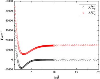
Figure 1. The ab initio energy points for the ${\rm{X}}{}^{{\rm{1}}}{\rm{\Sigma }}_{g}^{+}$ and ${\rm{A}}{}^{{\rm{1}}}{\rm{\Sigma }}_{u}^{+}$ states of the lithium dimer under the calculation of MRCI/AV5Z. |
We obtain the APEFs of the ground and first excited states of Li2 by fitting the ab initio energy points to equation (1 ) with the fitting term number of n = 11. The fitting parameters for the PECs based on the ab initio energy points of AVTZ, AVQZ, and AV5Z are presented in table 1, respectively. Re for the three sets of ab initio data are close to each other for the ${\rm{X}}{}^{{\rm{1}}}{\rm{\Sigma }}_{g}^{+}$ state. However, De presents significant difference between the AVTZ and the AVQZ data (∼80 cm−1), while De for AVQZ and AV5Z are much closer (∼14 cm−1). Thus, out of the three bases, AV5Z is considered to be the most suitable for the lithium dimer. The corresponding fitting results for the ${\rm{A}}{}^{{\rm{1}}}{\rm{\Sigma }}_{u}^{+}$ state with AV5Z basis set are listed in the last column of table 1. As shown in figure 2, the fitting curves for both the ground and excited states can well pass through all the ab initio energy points and the fitting curves are smooth with the variation of R. The adiabatic excitation energy (Te) is 13 986.2 cm−1 which is close to the previous experimental report (14 068 cm−1) [30]. The atomic excitation energy (Ea) is 14 849.2 cm−1 compared to the experiment (14 903 cm−1) [31].
Table 1. The fitting parameters of the MS analytical potential energy functions for the ${\rm{X}}{}^{{\rm{1}}}{\rm{\Sigma }}_{g}^{+}$ state based on MRCI/AVXZ (X = T, Q, 5) and the ${\rm{A}}{}^{{\rm{1}}}{\rm{\Sigma }}_{u}^{+}$ state based on MRCI/AV5Z. The corresponding ab initio calculation values for Re and De are listed in the parentheses. |
| Potential parameters | AVTZ ${\rm{X}}{}^{{\rm{1}}}{\rm{\Sigma }}_{g}^{+}$ | AVQZ ${\rm{X}}{}^{{\rm{1}}}{\rm{\Sigma }}_{g}^{+}$ | AV5Z ${\rm{X}}{}^{{\rm{1}}}{\rm{\Sigma }}_{g}^{+}$ | AV5Z ${\rm{A}}{}^{{\rm{1}}}{\rm{\Sigma }}_{u}^{+}$ |
|---|---|---|---|---|
| Re/Å | 2.6994 (2.6989) | 2.6976 (2.6978) | 2.6974 (2.6977) | 3.1421 (3.1401) |
| De/cm−1 | 8337.5346 (8338.6302) | 8414.9678 (8416.1149) | 8428.0893 (8429.2647) | 9291.0809 (9290.2886) |
| a1/Å−1 | 2.1776 | 2.1742 | 2.1729 | 1.5266 |
| a2/Å−2 | 1.6309 | 1.6239 | 1.6214 | 0.8087 |
| a3/Å−3 | 0.6373 | 0.6320 | 0.6305 | 0.2635 |
| a4/Å−4 | 0.1171 | 0.1149 | 0.1146 | 0.05164 |
| a5/Å−5 | −0.027 57 | −0.028 35 | −0.028 30 | 0.009 509 |
| a6/Å−6 | −0.014 67 | −0.014 37 | −0.014 34 | 0.000 7928 |
| a7/Å−7 | 0.002 564 | 0.002 635 | 0.002 566 | −0.002 086 |
| a8/Å−8 | 0.001 453 | 0.001 395 | 0.001 388 | 0.000 1562 |
| a9/Å−9 | 0.000 1205 | 0.000 1292 | 0.000 1395 | 0.000 2391 |
| a10/Å−10 | −0.000 1254 | −0.000 1253 | −0.000 1269 | −0.000 050 66 |
| a11/Å−11 | 0.000 013 69 | 0.000 013 57 | 0.000 013 62 | 0.000 003 274 |
| RMS/cm−1 | 0.7672 | 0.8006 | 0.8166 | 2.7880 |
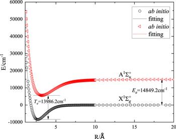
Figure 2. Ab initio points and fitting curves for the ${\rm{X}}{}^{{\rm{1}}}{\rm{\Sigma }}_{g}^{+}$ and ${\rm{A}}{}^{{\rm{1}}}{\rm{\Sigma }}_{u}^{+}$ states of Li2 under MRCI/AV5Z; Ea is the atomic excitation energy and Te is the adiabatic excitation energy. |
To further illustrate the validity of the MS fitting functions, we present the fitting error for each energy point in figure 3. Here, we compared two kinds of fittings: one is to set the term number n in the fitting function of equation (1 ) to be 9, and the other is to set n = 11. Obviously, with the increase of the term number, the fitting error decreases dramatically. The root means square (rms) errors can be calculated as ${\rm{RMS}}=\sqrt{\tfrac{1}{N}\displaystyle {\sum }_{i=1}^{N}{\left({V}_{{\rm{APEF}}}-{V}_{ab\,initio}\right)}^{2}},$ where N is the number of the data. As shown in figures 3(a) and (b), for n = 9, the rms = 3.0284 cm−1 for the ${\rm{X}}{}^{{\rm{1}}}{\rm{\Sigma }}_{g}^{+}$ state is smaller than that (rms) for the ${\rm{A}}{}^{{\rm{1}}}{\rm{\Sigma }}_{u}^{+}$ state. The distribution of the fitting error with the variation of R is also different between the two electronic states. The fitting error for the ${\rm{X}}{}^{{\rm{1}}}{\rm{\Sigma }}_{g}^{+}$ state is large for the short R region (R < 2 Å) with the largest error of roughly 14 cm−1, while the fitting for the ${\rm{A}}{}^{{\rm{1}}}{\rm{\Sigma }}_{u}^{+}$ state presents large errors (∼40 cm−1) in both the short R region (R < 2 Å) and the asymptote region (R > 10 Å). This is because that the potential energy varies drastically in the short R region for both electronic states, and that potential energy of the ${\rm{A}}{}^{{\rm{1}}}{\rm{\Sigma }}_{u}^{+}$ state presents a relatively long-range interaction to approaching the asymptote limit than the ${\rm{X}}{}^{{\rm{1}}}{\rm{\Sigma }}_{g}^{+}$ state does. Nevertheless, the fitting error can be declined by increasing the fitting terms n. As shown in figures 3(c) and (d), for n = 11, the fitting errors for both states in all R region are appreciably smaller than those for n = 9. The fitting error for the ${\rm{X}}{}^{{\rm{1}}}{\rm{\Sigma }}_{g}^{+}$ state for the short R region (R < 2 Å) has been decreased to within roughly 4 cm−1. The fitting errors for the ${\rm{A}}{}^{{\rm{1}}}{\rm{\Sigma }}_{u}^{+}$ state in the short R region (R < 2 Å) and the asymptote region (R > 10 Å) are now decreased to within 5 cm−1 and 10 cm−1, respectively. These errors are actually considerable small compared to the deep well depths of the two states (De = 8428 cm−1 for ${\rm{X}}{}^{{\rm{1}}}{\rm{\Sigma }}_{g}^{+}$ and De = 9291 cm−1 for ${\rm{A}}{}^{{\rm{1}}}{\rm{\Sigma }}_{u}^{+}$). In addition, the fitting errors for the two states at the equilibrium Re are both extremely small (1.176 cm−1 for ${\rm{X}}{}^{{\rm{1}}}{\rm{\Sigma }}_{g}^{+}$ and 0.7788 cm−1 for ${\rm{A}}{}^{{\rm{1}}}{\rm{\Sigma }}_{u}^{+}$). The rms errors for n = 11 and for different basis sets are also listed in table 1. The rms is 0.8166 cm−1 for the ${\rm{X}}{}^{{\rm{1}}}{\rm{\Sigma }}_{g}^{+}$ state in our fitting to MRCI/AV5Z. Even for the ${\rm{A}}{}^{{\rm{1}}}{\rm{\Sigma }}_{u}^{+}$ state, the rms is only 2.788 cm−1 which is much smaller than the permitted chemical accuracy (1.0 kcal mol−1 or 349.755 cm−1) and proves the high quality of the fitting process. The small fitting error also indicates that the MS function is suitable for the description of the ground and first excited states of Li2.
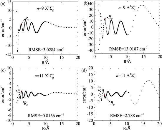
Figure 3. Fitting errors of the PECs for the ground state (a) and the first state (b) of Li2 with n = 9; fitting errors of the PECs for the ground state (c) and the first state (d) of Li2 with n = 11. |
Hereinbefore, we demonstrate the fitting process and determine the APEFs with n = 11 based on the energy points calculated by MRCI/AV5Z. Now, we further compare the highly accurate fitting functions with previous reported spectroscopic constants in theory and experiment. The comparison for the ${\rm{X}}{}^{{\rm{1}}}{\rm{\Sigma }}_{g}^{+}$ state is shown in table 2. Obviously, the values calculated from our APEFs, including the spectroscopic constants, equilibrium bond lengths Re (Å), and potential well depth De (cm−1) are all in good agreement with the experiments [21, 30], compared with previous theoretical reports [14, 18, 19, 33, 34, 38, 39]. The spectroscopic constants, equilibrium bond lengths Re, and potential well depth De of the first excited state ${\rm{A}}{}^{{\rm{1}}}{\rm{\Sigma }}_{u}^{+}$ are shown in table 3. It can be seen that the fitting APEFs for the excited state can also present accurate spectroscopic constants in good agreement with experimental and theoretical reports [14, 18, 32–34, 36, 40]. Thus, these APEFs based on MRCI/AV5Z for the ground and first excited states of the Li2 dimer are reliable for future studies in spectroscopy and molecular dynamics.
Table 2. Equilibrium bond lengths Re (Å), potential well depth De (cm−1) and spectroscopic constants (cm−1) for the ground state ${\rm{X}}{}^{{\rm{1}}}{\rm{\Sigma }}_{g}^{+}$ of Li2. |
| Basis/References | Re/Å | De/cm−1 | ωe/cm−1 | Be/cm−1 | ωeχe/cm−1 | αe/cm−1 |
|---|---|---|---|---|---|---|
| AV5Z | 2.6974 | 8428.089 | 347.9251 | 0.661 04 | 2.4932 | 0.006 956 |
| Exp. [21] | 2.6734 | 8549.473 | 351.422 95 | 0.668 24 | 2.4417 | — |
| Exp. [30] | 2.673 | 8549.473 | 351.4 | 0.673 | 2.61 | 0.0068 |
| Theory [18] | 2.658 | 8613 | 352.41 | — | — | — |
| Theory [34] | 2.660 | 8510 | 353.0 | — | — | — |
| Theory [35] | 2.675 | 8466 | 351.01 | — | — | — |
| Theory [19] | 2.752 | 7856.64 | 352.50 | 0.675 | 2.70 | — |
| Theory [14] | 2.677 | 8466 | 351.0 | — | — | — |
| Theory [38] | 2.677 | 8065.541 | 351.9 | 0.671 | 2.56 | 0.0073 |
| Theory [39] | 2.7146 | 7307.38 | 327.50 | 0.668 24 | 2.651 47 | 0.006 50 |
| Theory [33] | 2.692 | 8297 | 347.1 | — | 3.6 | — |
Table 3. Equilibrium bond lengths Re (Å), potential well depth De (cm−1) and spectroscopic constants (cm−1) for the state ${\rm{A}}{}^{{\rm{1}}}{\rm{\Sigma }}_{u}^{+}$ of Li2. |
| Basis/References | Re/Å | De/cm−1 | ωe/cm−1 | Be/cm−1 | ωeχe/cm−1 | αe/cm−1 |
|---|---|---|---|---|---|---|
| AV5Z | 3.142 | 9291.0809 | 253.704 | 0.487 | 1.511 | 0.005 02 |
| Exp. [32] | 3.108 | 9353.6079 | 255.47 | 0.498 | 1.581 | 0.005 48 |
| Theory [36] | 3.133 | 9366.5127 | 251.97 | 0.490 | 1.623 | 0.005 35 |
| Theory [34] | 3.094 | 9466 | 257.4 | — | — | — |
| Theory [33] | 3.13 | 9299 | 254 | — | 1.7 | — |
| Theory [40] | 3.072 | 9651.226 | 261.3 | — | 1.77 | — |
| Theory [14] | 3.112 | 9356 | 255 | — | — | — |
| Theory [18] | 3.092 | 9483 | 257.54 | — | — | — |
3.2. Vibrational levels and FCF
Based on this newly constructed APEFs, we further calculated the vibrational energy levels by solving the following time-independent Schrödinger equation of nuclear motion using the Fourier grid Hamilton method [37].
$\begin{eqnarray}\begin{array}{l}\left[-\displaystyle \frac{{\hslash }^{2}}{2\mu }\displaystyle \frac{{{\rm{d}}}^{2}}{{\rm{d}}{R}^{2}}+\displaystyle \frac{j(j+1){\hslash }^{2}}{2\mu {R}^{2}}+{V}^{\left(i\right)}(R)\right]{{\psi }^{\left(i\right)}}_{v,j}(R)\\ \,={{E}^{\left(i\right)}}_{v,j}{{\psi }^{\left(i\right)}}_{v,j}(R),\end{array}\end{eqnarray}$
where μ is reduced mass, j is rotational quantum number, v is vibrational quantum number, and V(i)(R) is the APEF of the ith electronic state, i = ${\rm{X}}{}^{{\rm{1}}}{\rm{\Sigma }}_{g}^{+}$ and ${\rm{A}}{}^{{\rm{1}}}{\rm{\Sigma }}_{u}^{+}.$Within the R range from 1.2 to 20 Å, we use 1024 grid points in the computation of the vibrational levels of the ground and first excited states of the lithium dimer. The density of the grid points has been checked to be converged by using even denser grids. The obtained vibrational levels (with j = 0) of the ground state of 7Li2, 6Li2, and 6Li7Li are listed in table 4, where δ is the relative difference between the present calculation and the previous experiment measurement [21]. The ground vibrational level of the ${\rm{X}}{}^{{\rm{1}}}{\rm{\Sigma }}_{g}^{+}$ state is close to the experimental result with the rather small difference of 1 cm−1. The relative difference δ for every vibrational level is less than 1.5%. In general, the APEF of the ground state of Li2 from equation (1 ) is reliable. Due to the decrease of the reduced mass, the number of vibrational levels for 6Li2 (6Li7Li) is smaller than that for 7Li2, and for given vibrational level, the eigenenergy for the 6Li2 (6Li7Li) dimer is higher than that for the 7Li2 dimer.
Table 4. The eigenenergies of vibrational levels for the ground state ${\rm{X}}{}^{{\rm{1}}}{\rm{\Sigma }}_{g}^{+}$ of Li2, relative to the bottom of the potential well (cm−1). |
| Vibrational levels | 7Li2 | Exp. of 7Li2 [21] | δ | 6Li2 | 6Li7Li |
|---|---|---|---|---|---|
| 0 | 173.945 07 | 175.032 | 0.62% | 180.945 46 | 187.679 75 |
| 1 | 514.991 96 | 521.2611 | 1.20% | 535.682 43 | 555.5745 |
| 2 | 851.009 63 | 862.2642 | 1.31% | 884.9692 | 917.597 74 |
| 3 | 1181.955 78 | 1197.9974 | 1.34% | 1228.757 25 | 1273.694 39 |
| 4 | 1507.7793 | 1528.4128 | 1.35% | 1566.987 78 | 1623.797 43 |
| 5 | 1828.420 39 | 1853.4573 | 1.35% | 1899.5918 | 1967.8281 |
| 6 | 2143.810 68 | 2173.0721 | 1.35% | 2226.490 22 | 2305.695 88 |
| 7 | 2453.873 11 | 2487.1914 | 1.34% | 2547.593 81 | 2637.298 48 |
| 8 | 2758.521 94 | 2795.7419 | 1.33% | 2862.803 03 | 2962.521 61 |
| 9 | 3057.6625 | 3090.6412 | 1.07% | 3172.007 88 | 3281.238 74 |
| 10 | 3351.191 03 | 3395.7978 | 1.31% | 3475.087 47 | 3593.310 57 |
| 11 | 3638.994 29 | 3687.1094 | 1.30% | 3771.909 67 | 3898.584 58 |
| 12 | 3920.949 17 | 3972.4624 | 1.30% | 4062.330 54 | 4196.894 17 |
| 13 | 4196.922 17 | 4251.7309 | 1.29% | 4346.193 57 | 4488.057 89 |
| 14 | 4466.768 81 | 4524.7756 | 1.28% | 4623.328 95 | 4771.878 24 |
| 15 | 4730.3328 | 4791.4274 | 1.28% | 4893.552 49 | 5048.140 41 |
| 16 | 4987.445 23 | 5051.5343 | 1.27% | 5156.664 47 | 5316.610 74 |
| 17 | 5237.923 51 | 5304.9322 | 1.26% | 5412.448 22 | 5577.034 79 |
| 18 | 5481.570 11 | 5551.3992 | 1.26% | 5660.668 47 | 5829.135 24 |
| 19 | 5718.171 18 | 5790.7056 | 1.25% | 5901.069 42 | 6072.609 25 |
| 20 | 5947.494 87 | 6022.6578 | 1.25% | 6133.372 45 | 6307.1254 |
| 21 | 6169.289 37 | 6246.9482 | 1.24% | 6357.2735 | 6532.320 18 |
| 22 | 6383.280 71 | 6463.314 | 1.24% | 6572.439 91 | 6747.793 77 |
| 23 | 6589.170 09 | 6671.3979 | 1.23% | 6778.506 85 | 6953.105 17 |
| 24 | 6786.6309 | 6870.8931 | 1.23% | 6975.073 19 | 7147.766 69 |
| 25 | 6975.305 31 | 7061.4199 | 1.22% | 7161.696 76 | 7331.237 74 |
| 26 | 7154.8003 | 7242.5556 | 1.21% | 7337.889 15 | 7502.918 41 |
| 27 | 7324.6835 | 7413.8431 | 1.20% | 7503.110 37 | 7662.143 36 |
| 28 | 7484.478 69 | 7574.8736 | 1.19% | 7656.763 83 | 7808.178 19 |
| 29 | 7633.661 69 | 7724.9165 | 1.18% | 7798.193 26 | 7940.221 94 |
| 30 | 7771.657 56 | 7863.7083 | 1.17% | 7926.684 64 | 8057.423 82 |
| 31 | 7897.841 32 | 7990.4162 | 1.16% | 8041.479 | 8158.929 24 |
| 32 | 8011.546 26 | 8104.473 | 1.15% | 8141.807 58 | 8243.978 73 |
| 33 | 8112.0875 | 8205.2323 | 1.14% | 8226.966 99 | 8312.078 42 |
| 34 | 8198.813 46 | 8292.0293 | 1.12% | 8296.4519 | 8363.196 |
| 35 | 8271.200 14 | 8364.3066 | 1.11% | 8350.124 34 | 8397.803 78 |
| 36 | 8328.9873 | 8421.6123 | 1.10% | 8388.2943 | 8417.116 82 |
| 37 | 8372.291 21 | 8463.9648 | 1.08% | 8411.709 99 | 8425.784 12 |
| 38 | 8401.576 36 | — | — | 8423.144 09 | — |
| 39 | 8418.019 85 | — | — | 8427.9374 | — |
| 40 | 8425.784 71 | — | — | — | — |
The vibrational levels (with j = 0) of the first excited state ${\rm{A}}{}^{{\rm{1}}}{\rm{\Sigma }}_{u}^{+}$ of Li2 are listed in table 5. The differences between our calculations and the previous experimental reports for the vibrational levels of the ${\rm{A}}{}^{{\rm{1}}}{\rm{\Sigma }}_{u}^{+}$ state are within 1.5%. Thus, the fitting APEFs for the two electronic states can also well describe the corresponding vibrational levels.
Table 5. The eigenenergies of vibrational levels for the ground state ${\rm{A}}{}^{{\rm{1}}}{\rm{\Sigma }}_{u}^{+}$ of Li2, relative to the bottom of the potential well (cm−1). |
| Vibrational levels | 7Li2 | Exp. of 7Li2 [11] | δ | Vibrational levels | 7Li2 | Exp. of 7Li2 [11] | δ |
|---|---|---|---|---|---|---|---|
| 0 | 127.568 43 | 127.2989 | 0.21% | 38 | 7428.303 59 | 7490.7088 | 0.83% |
| 1 | 376.880 56 | 379.5847 | 0.72% | 39 | 7552.610 13 | 7614.4744 | 0.81% |
| 2 | 623.157 98 | 628.7628 | 0.90% | 40 | 7672.434 98 | 7733.6054 | 0.79% |
| 3 | 866.395 79 | 874.8276 | 0.97% | 41 | 7787.653 52 | 7847.9802 | 0.77% |
| 4 | 1106.592 87 | 1117.7878 | 1.01% | 42 | 7898.142 05 | 7957.4828 | 0.75% |
| 5 | 1343.751 17 | 1357.6575 | 1.03% | 43 | 8003.781 36 | 8062.0058 | 0.72% |
| 6 | 1577.875 08 | 1594.4510 | 1.05% | 44 | 8104.461 43 | 8161.4558 | 0.70% |
| 7 | 1808.9708 | 1828.1805 | 1.06% | 45 | 8200.087 59 | 8255.7576 | 0.67% |
| 8 | 2037.045 63 | 2058.8553 | 1.07% | 46 | 8290.588 05 | 8344.8591 | 0.65% |
| 9 | 2262.107 44 | 2286.4820 | 1.08% | 47 | 8375.922 57 | 8428.7364 | 0.63% |
| 10 | 2484.163 98 | 2511.0647 | 1.08% | 48 | 8456.091 23 | 8507.398 | 0.60% |
| 11 | 2703.222 39 | 2732.6056 | 1.09% | 49 | 8531.141 77 | 8580.8882 | 0.58% |
| 12 | 2919.288 62 | 2951.1052 | 1.09% | 50 | 8601.173 15 | 8649.2902 | 0.56% |
| 13 | 3132.366 96 | 3166.5620 | 1.09% | 51 | 8666.3329 | 8712.7268 | 0.53% |
| 14 | 3342.459 56 | 3378.9730 | 1.09% | 52 | 8726.807 05 | 8771.36 | 0.51% |
| 15 | 3549.566 06 | 3588.3326 | 1.09% | 53 | 8782.803 46 | 8825.3883 | 0.48% |
| 16 | 3753.683 18 | 3794.6329 | 1.09% | 54 | 8834.532 03 | 8875.0421 | 0.46% |
| 17 | 3954.804 38 | 3997.8627 | 1.09% | 55 | 8882.186 98 | 8920.5765 | 0.43% |
| 18 | 4152.919 62 | 4198.0072 | 1.09% | 56 | 8925.936 07 | 8962.2626 | 0.41% |
| 19 | 4348.015 | 4395.0479 | 1.08% | 57 | 8965.920 77 | 9000.3768 | 0.38% |
| 20 | 4540.0726 | 4588.9617 | 1.08% | 58 | 9002.270 19 | 9035.1898 | 0.36% |
| 21 | 4729.070 25 | 4779.7214 | 1.07% | 59 | 9035.130 82 | 9066.9562 | 0.35% |
| 22 | 4914.9813 | 4967.2950 | 1.06% | 60 | 9064.709 43 | 9095.9063 | 0.34% |
| 23 | 5097.774 47 | 5151.6462 | 1.06% | 61 | 9091.312 89 | 9122.2439 | 0.34% |
| 24 | 5277.413 68 | 5332.7340 | 1.05% | 62 | 9115.350 98 | 9146.152 | 0.34% |
| 25 | 5453.857 92 | 5510.5127 | 1.04% | 63 | 9137.277 51 | — | — |
| 26 | 5627.061 02 | 5684.9326 | 1.03% | 64 | 9157.499 54 | — | — |
| 27 | 5796.971 59 | 5855.9387 | 1.02% | 65 | 9176.317 07 | — | — |
| 28 | 5963.532 81 | 6023.4718 | 1.01% | 66 | 9193.9154 | — | — |
| 29 | 6126.6823 | 6187.4674 | 0.99% | 67 | 9210.385 97 | — | — |
| 30 | 6286.352 01 | 6347.8558 | 0.98% | 68 | 9225.749 96 | — | — |
| 31 | 6442.468 | 6504.5615 | 0.96% | 69 | 9239.974 11 | — | — |
| 32 | 6594.950 43 | 6657.503 | 0.95% | 70 | 9252.977 34 | — | — |
| 33 | 6743.713 35 | 6806.5922 | 0.93% | 71 | 9264.627 73 | — | — |
| 34 | 6888.664 74 | 6951.7343 | 0.92% | 72 | 9274.726 95 | — | — |
| 35 | 7029.706 44 | 7092.828 | 0.90% | 73 | 9282.969 81 | — | — |
| 36 | 7166.734 29 | 7229.7651 | 0.88% | 74 | 9288.831 93 | — | — |
| 37 | 7299.6384 | 7362.4316 | 0.86% | — | — | — | — |
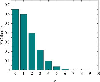
Based on the obtained vibrational level v′ = 0 of the ground state and all the bound vibrational levels of the ${\rm{A}}{}^{{\rm{1}}}{\rm{\Sigma }}_{u}^{+}$ state of Li2, we calculate the corresponding FCFs, $\left\langle {{\rm{\Psi }}}_{v^{\prime} ={\rm{0}}}^{X}\left|{{\rm{\Psi }}}_{v^{\prime\prime} =0}^{A}\right.\right\rangle ,$ which are illustrated in figure 4 and the specific values are listed in table 6. As seen in figure 4 and table 6, the maximum FCF corresponds to the overlap between v′ = 0 and v″ = 0, and the value of FCF decreases dramatically with the increase of the vibrational quantum number v″ of the excited state. For v″ greater than 7, one cannot figure out its contribution from figure 4. It is because that the equilibriums for the PECs of the two electronic states are similar, roughly 2.7 and 3.1 Å and that the width and depth of the two potential wells are also comparable. Thus, the ground vibrational wavefunctions for two electronic states are similar in shape and position, which can present the largest FCF.
Table 6. Franck–Condon factors for the transition from the v′ = 0 of the ${\rm{X}}{}^{{\rm{1}}}{\rm{\Sigma }}_{g}^{+}$ state to the v″ = 0–74 of the ${\rm{A}}{}^{{\rm{1}}}{\rm{\Sigma }}_{u}^{+}$ state of 7Li2. |
| v″ | F–C factors | v″ | F–C factors |
|---|---|---|---|
| 0 | 0.651 42 | 38 | 1.54E-10 |
| 1 | 0.600 29 | 39 | 7.65E-11 |
| 2 | 0.397 16 | 40 | 2.91E-11 |
| 3 | 0.214 89 | 41 | 2.24E-12 |
| 4 | 0.0988 | 42 | 1.16E-11 |
| 5 | 0.038 41 | 43 | 1.76E-11 |
| 6 | 0.0118 | 44 | 1.90E-11 |
| 7 | 0.002 01 | 45 | 1.81E-11 |
| 8 | 7.04E-04 | 46 | 1.61E-11 |
| 9 | 9.70E-04 | 47 | 1.38E-11 |
| 10 | 6.45E-04 | 48 | 1.15E-11 |
| 11 | 3.26E-04 | 49 | 9.41E-12 |
| 12 | 1.31E-04 | 50 | 7.63E-12 |
| 13 | 3.68E-05 | 51 | 6.15E-12 |
| 14 | 4.70E-07 | 52 | 4.94E-12 |
| 15 | 9.01E-06 | 53 | 3.97E-12 |
| 16 | 8.53E-06 | 54 | 3.18E-12 |
| 17 | 5.65E-06 | 55 | 2.56E-12 |
| 18 | 3.07E-06 | 56 | 2.06E-12 |
| 19 | 1.39E-06 | 57 | 1.66E-12 |
| 20 | 4.78E-07 | 58 | 1.34E-12 |
| 21 | 6.11E-08 | 59 | 1.09E-12 |
| 22 | 8.77E-08 | 60 | 8.90E-13 |
| 23 | 1.13E-07 | 61 | 7.30E-13 |
| 24 | 9.23E-08 | 62 | 6.10E-13 |
| 25 | 6.23E-08 | 63 | 5.10E-13 |
| 26 | 3.69E-08 | 64 | 4.30E-13 |
| 27 | 1.92E-08 | 65 | 3.70E-13 |
| 28 | 8.43E-09 | 66 | 3.10E-13 |
| 29 | 2.55E-09 | 67 | 2.70E-13 |
| 30 | 2.49E-10 | 68 | 2.30E-13 |
| 31 | 1.31E-09 | 69 | 1.90E-13 |
| 32 | 1.49E-09 | 70 | 1.60E-13 |
| 33 | 1.29E-09 | 71 | 1.40E-13 |
| 34 | 9.87E-10 | 72 | 1.10E-13 |
| 35 | 6.91E-10 | 73 | 9.00E-14 |
| 36 | 4.51E-10 | 74 | 6.00E-14 |
| 37 | 2.75E-10 | — | — |
Figure 4. Franck–Condon factors for the transition from the v′ = 0 of the ${\rm{X}}{}^{{\rm{1}}}{\rm{\Sigma }}_{g}^{+}$ state to the v″ = 0–10 of the ${\rm{A}}{}^{{\rm{1}}}{\rm{\Sigma }}_{u}^{+}$ state of 7Li2. |
4. Conclusion
The PECs of the ${\rm{X}}{}^{{\rm{1}}}{\rm{\Sigma }}_{g}^{+}$ and ${\rm{A}}{}^{{\rm{1}}}{\rm{\Sigma }}_{u}^{+}$ states of Li2 have been calculated by MRCI method based on different basis sets AVTZ, AVQZ, and AV5Z.
Based on the comparison among the three basis sets, we perform the nonlinear least square fitting to the MRCI/AV5Z energy points with MS potential energy function. The rms errors for the ${\rm{X}}{}^{{\rm{1}}}{\rm{\Sigma }}_{g}^{+}$ and ${\rm{A}}{}^{{\rm{1}}}{\rm{\Sigma }}_{u}^{+}$ states are 0.8166 cm−1 and 2.788 cm−1, respectively. The equilibrium distance, potential well depth, spectroscopic constants, and vibrational energy levels described by the two APEFs are in good agreement with the experimental reports. The FCFs corresponding to the transitions from the vibrational level (v′ = 0) of the ground state to the vibrational levels (v″ = 0–74) of the first excited state have been calculated, which indicates that the vibronic transition from ${\rm{X}}{}^{{\rm{1}}}{\rm{\Sigma }}_{g}^{+}$ (v′ = 0) to ${\rm{A}}{}^{{\rm{1}}}{\rm{\Sigma }}_{u}^{+}$(v″ = 0) is the strongest. These two accurate APEFs provide a theoretical basis for future studies in spectroscopy and molecular dynamics of the Li2 dimer.