


1. Introduction
There has been a great revival of out-of-time-ordered correlation (OTOC) functions in recent years. Its importance was first realized by A Larkin and Y N Ovchinnikov [1]. After several decades of silence, its relevance to black holes was revealed by A Y Kitaev [2, 3]. Consider two generic unitary operators V and W, along with the Hamiltonian H of a many-body system. The OTOC is defined as
$\begin{eqnarray}F(t)=\displaystyle \frac{1}{2}\left(\langle {V}^{\dagger }(0){W}^{\dagger }(t)V(0)W(t)\rangle +{\rm{h}}.{\rm{c}}.\right),\end{eqnarray}$
where V(0) = V and W(t) = eiHtWe−iHt denote time-evolving unitary operators. ⟨...⟩ stands for the expectation value on a pure state of interest (in our case the ground state), or the thermal average for a given temperature. The OTOC is closely related to the squared commutator of V and W(t), which is written as C(t) = ⟨∣[W(t), V]∣2⟩ = 2(1 − ReF(t)). Naively substituting $W=V=\hat{p}$, we have [4] $\begin{eqnarray}\begin{array}{l}C(t)={{\hslash }}^{2}\left\langle {\left(\displaystyle \frac{\partial \hat{p}(t)}{\partial x(0)}\right)}^{2}\right\rangle \\ \approx \,{{\hslash }}^{2}\left\langle \left\langle {\left(\displaystyle \frac{{\rm{\Delta }}p(t)}{{\rm{\Delta }}x(0)}\right)}^{2}\right\rangle \right\rangle ={C}_{\mathrm{cl}}(t),\end{array}\end{eqnarray}$
where $\hat{p}$ and $\hat{x}$ are the momentum and position operators, Ccl(t) is the classical counterpart of C(t). Then, we can see the intrinsic relation of C(t) with classical chaos, which attracts a lot of interest [5–8]. Over years of studies, OTOC is proved to be powerful in different scenarios including many-body localization, [9–11] information scrambling [12] and AdS/CFT [8, 13, 14].As theoretical studies on OTOC go on, [15–19] direct computations show that it can be used as an order parameter to distinguish different quantum phases. There have been flourishing works on the 1D Bose–Hubbard model, [20] Ising model [21] and the XXZ model [22]. In reference [23], OTOC in the Lipkin-Meshkov-Glick model is researched, indicating some connections between OTOC and excited-state quantum phase transition. Even in the topological phase transition, OTOC has a substantial footprint [24].
The Dicke model is definitely a fundamental model of cavity-QED, describing the interaction of many atoms to a single cavity mode [25–28]. This model undergoes a phase transition to a superradiant state at a critical value of the atom-field interaction [26]. Classical chaos methods are widely applied to this model even before the recent enthusiasm [25, 26, 29–34]. In reference [35], a diagrammatic method on OTOC is used to compute the Lyapunov exponent and study the chaotic behavior of the Dicke model. Reference [34] shows OTOCs of the Dicke model can also grow exponentially in its non-chaotic regime. The interplay of quantum phase transition and chaos remains an open question. Using OTOC as a complementary tool to show ergodic-nonergodic transition in a generalized version of the Dicke model, reference [36] concludes the existence of a quantum analogue of the classical Kolmogorov-Arnold-Moser (KAM) theorem, [37, 38] which might be misleading because the OTOC fails to show its power in detecting quantum phase transition.
In this work, we compute OTOC in the anisotropic Dicke model. Since the rigid quantum phase transition only occurs at zero temperature, we focus on zero temperature OTOC. Here, we recover the phase diagram of the anisotropic Dicke model with OTOC and study the finite-size effect. Finally, we give the dynamical pattern of OTOC as the temperature increases.
2. The model and the main result
The anisotropic Dicke model (ADM) can be written as
$\begin{eqnarray}\begin{array}{rcl}H&=&{\hslash }\omega {a}^{\dagger }a+{\hslash }{\omega }_{z}{J}_{z}+\displaystyle \frac{{g}_{1}}{\sqrt{2j}}\left({a}^{\dagger }{J}_{-}+{{aJ}}_{+}\right)\\ & & +\ \displaystyle \frac{{g}_{2}}{\sqrt{2j}}\left({a}^{\dagger }{J}_{+}+{{aJ}}_{-}\right),\end{array}\end{eqnarray}$
where a(a†) are bosonic annihilation (creation) operators, satisfying [a, a†] = 1 and ${J}_{\pm ,z}={\sum }_{i=1}^{2j}\tfrac{1}{2}{\sigma }_{\pm ,z}^{(i)}$ are angular momentum operators, describing a pseudospin of length j composed of N = 2j non-interacting spin-1/2 atoms described by the Pauli matrices ${\sigma }_{\pm ,z}^{(i)}$ acting on site i. The ADM describes a single bosonic mode (often a cavity photon mode) of frequency ω which interacts collectively with a set of N two-level systems (the atoms) with energy-splitting ωz (ℏ conventionally taken to be 1), within the dipole approximation coupled to the field. Written in terms of collective operators, the ADM can be dramatically simplified when we take j to have its maximal value j = N/2. The model has four tunable parameters: The photon frequency ω, the atomic energy splitting ωz and counter-(co-)rotating photon-atom coupling g1(g2). For g1 = g2 = g, the ADM reduces to the Dicke model with coupling parameter g. The ADM possesses a parity symmetry ${\rm{\Pi }}=\exp (i\pi [{a}^{\dagger }a+{J}_{z}+j])$ satisfying [H, Π] = 0 with eigenvalues±1.Our focus is restricted to the positive parity subspace, which includes the ground state for the parameter ranges considered in this work [26]. Hereafter, we work in the basis {∣n⟩ ⨂ ∣j, m⟩} with a†a∣n⟩ = n∣n⟩ and Jz∣j, m⟩ = m∣j, m⟩ and we set ω = ωz = 1 which is most physically acceptable. We take the cutoff of the number of bosons to be 100 unless otherwise stated (i.e. ncutoff = 100).
When g1 = 0 or g2 = 0, the ADM is integrable, which inspires a lot of researchers working on the integrablity of the model. In the thermodynamic limit N → ∞ , the ADM exhibits a second-order quantum phase transition at ${g}_{1}+{g}_{2}=\sqrt{\omega {\omega }_{z}}$ with order parameter a†a/j, [26] separating the normal phase at ${g}_{1}+{g}_{2}\lt \sqrt{\omega {\omega }_{z}}$ with ⟨a†a⟩/j = 0 from the superradiant phase with $\langle {a}^{\dagger }a\rangle /j={ \mathcal O }(1)$.
In the following, we utilize OTOC to detect the phase transition in the ADM. We take W = V = a†a + 10, N = 2j = 10, and compute the OTOC at zero temperature, i.e. F(t) = ⟨V†W†(t)VW(t)⟩, where ⟨...⟩ stands for the expectation value on ground state. We focus on R(t) = 1 − F(t)/F(0). This value, dubbed residue OTOC, is large if the system spreads information fast. For a generic system, it is generally close to zero. In figure 1, R(t) is plotted for typical g1,2, as a function of time, from which we can see the OTOC of the ADM shows steady behavior.
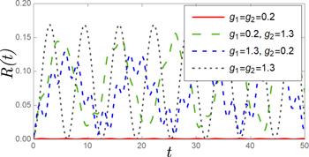
Figure 1. The representative time evolution of R(t) (defined in the text). |
This enables us to utilize $\bar{{ \mathcal R }}={\mathrm{lim}}_{t\to \infty }{\int }_{0}^{t}R(t^{\prime} ){\rm{d}}t^{\prime} $, which is considered as saturation value, [22] to separate different phases. As indicated in figure 2, in normal phase (blue region), $\bar{{ \mathcal R }}$ is smaller than in the superradiant phase (white region), as a function of g1,2. In general, it is easy to understand that F(t) will not go far from F(0), if the interaction between atoms and field is small, leading to a small value of $\bar{{ \mathcal R }}$. We take about 30 × 30 points resulting in the saw-tooth pattern of the separatrix, which suggests the existence of a phase boundary. If more discrete points in the (g1, g2) space are considered, a smoother phase boundary is expected.
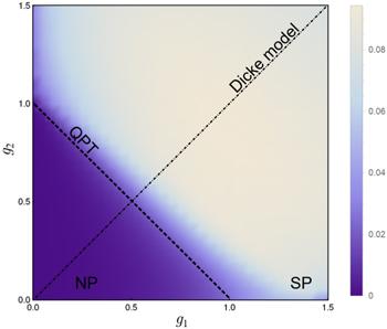
Figure 2. Density plot of $\bar{{ \mathcal R }}$ as a function of g1,2. The Dicke model, i.e. in which g1 = g2, is indicated by a dot-dashed line. Normal phase (NP) and superradiant phase (SP) are separated by the quantum phase transition (QPT) line, the dashed line. |
3. Finite-size effect and temperature going high
To analyze the finite-size effect with N increasing, we further calculate $\bar{{ \mathcal R }}$ with different N along the Dicke line as a function of g. Figure 3 shows close to the critical point (g ≈ 0.5), the slope is steeper with N larger. In the thermodynamic limit, we expect at gc = 0.5, there will be a sudden jump. Note that when N ≥ 6, there is a decreasing tendency with g going large. We believe it is caused by relatively small ncutoff, which does not have any effect on our discussion.
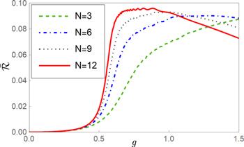
Figure 3. $\bar{{ \mathcal R }}$ as a function of the Dicke coupling constant g, plotted with different N (the size of the system). |
We plot the derivative of $\bar{{ \mathcal R }}$ with respect to g in figure 4. Despite the rapid oscillating behavior, we can infer there is a QPT near gc = 0.5.
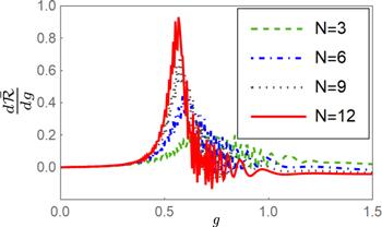
Figure 4. $\tfrac{{\rm{d}}\bar{{ \mathcal R }}}{{\rm{d}}g}$ plotted as g. The rapid oscillations are consequences of the finite time window we take. |
To provide more compelling evidence, we give three fittings with N increasing. In figure 5(a), both the value at gc and the maximum of $\tfrac{{\rm{d}}\bar{{ \mathcal R }}}{{\rm{d}}g}$ grow linearly with N, fitting models being −0.0071 + 0.0249N (red line) and −0.0046 + 0.0776N (blue line) respectively. In figure 5(b), we fit the data using aN−b + c, with a = 0.4079, b = 0.9220 and c = 0.0253.
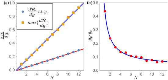
Figure 5. (a) Fittings of $\tfrac{{\rm{d}}\bar{{ \mathcal R }}}{{\rm{d}}g}$ at gc = 0.5 and of maximum of $\tfrac{{\rm{d}}\bar{{ \mathcal R }}}{{\rm{d}}g}$, respectively as a function of N. (b) Peak position gp minus gc as a function of N, tending to 0 with N large. Fitting models and parameters are given in the text. |
The fittings clearly show the existence of a jump of $\bar{{ \mathcal R }}$ at gc, in the thermodynamic limit.
It is believed that OTOC can characterize ergodic-nonergodic transition in the ADM, [36] but with a relatively high temperature (T = 10).
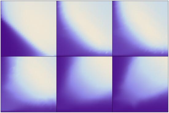
Here, we want to track how a single physical quantity can show quite different physics of a system. In figure 6, we plot $\bar{{ \mathcal R }}$ as a function of g1,2, with β being ∞, 1, 0.7, 0.3, 0.1, and 0, viz, temperature being 0, 1, 1.43, 3.33, 10 and ∞. Although the scalings are different, the patterns are rather smooth, varying from a relatively clear boundary, which shows the existence of QPT, to a relatively blurred one, which is considered as a hint of the quantum KAM theorem.
Figure 6. Density plot of $\bar{{ \mathcal R }}$ as a function of g1,2 with T = 0, 1, 1.43, 3.33, 10, ∞ respectively. Although the legends of each density plot are different, they do not matter and are left out for simplicity. |
4. Conclusion and discussion
In this work, we compute zero temperature OTOC in the anisotropic Dicke model, and recover the phase diagram, which possesses a clear boundary between the normal phase and the superradiant phase. Further finite-size effect is discussed, and in the thermodynamic limit, the saturation value of the residue OTOC in the Dicke model will be like a step function, which demonstrates that the boundary line in the ADM will be quite clear as the number of atoms goes to infinity. We also provide a dynamic changing of density plot of $\bar{{ \mathcal R }}$ as the temperature increases. At zero temperature, the boundary is clear and separates the superradiant phase from the normal phase; At a quantitatively high temperature (T ≥ 10), the boundary is fuzzy, which shows an ergodic-nonergodic transition, suggesting the rationality of the quantum Kolmogorov-Arnold-Moser theorem.