Welcome to visit Communications in Theoretical Physics,
Quantum Physics and Quantum Information

Quantum uncertainty relations of Tsallis relative α entropy coherence based on MUBs

  • Fu-Gang Zhang , *
Expand
  • School of Mathematics and Information Science, Nanchang Hangkong University, Nanchang 330063, China

*Author to whom any correspondence should be addressed.

Received date: 2021-07-09

  Revised date: 2021-12-11

  Accepted date: 2021-12-13

  Online published: 2022-02-09

Copyright

© 2022 Institute of Theoretical Physics CAS, Chinese Physical Society and IOP Publishing

Abstract

In this paper, we discuss quantum uncertainty relations of Tsallis relative α entropy coherence for a single qubit system based on three mutually unbiased bases. For $\alpha \in \left[\tfrac{1}{2},1\right)\cup (1,2]$, the upper and lower bounds of sums of coherence are obtained. However, the above results cannot be verified directly for any $\alpha \in \left(0,\tfrac{1}{2}\right)$. Hence, we only consider the special case of $\alpha =\tfrac{1}{n+1}$, where n is a positive integer, and we obtain the upper and lower bounds. By comparing the upper and lower bounds, we find that the upper bound is equal to the lower bound for the special $\alpha =\tfrac{1}{2}$, and the differences between the upper and the lower bounds will increase as α increases. Furthermore, we discuss the tendency of the sum of coherence, and find that it has the same tendency with respect to the different θ or φ, which is opposite to the uncertainty relations based on the Rényi entropy and Tsallis entropy.

Cite this article

Fu-Gang Zhang . Quantum uncertainty relations of Tsallis relative α entropy coherence based on MUBs[J]. Communications in Theoretical Physics, 2022 , 74(1) : 015102 . DOI: 10.1088/1572-9494/ac4264

1. Introduction

Quantum coherence derived from quantum superposition is one of the fundamental features of quantum mechanics. Quantum coherence resource theory plays an important role not only in the quantum theory but also in the practical application [14]. Quantifying the coherence of quantum states is one of the core tasks of quantum coherence resource theory. Baumgratz et al proposed a rigorous framework to quantify coherence [5]. The framework stipulated that a well coherence measure must fulfil several conditions.
Based on the framework, many suitable measures were put forward with respect to the fixed orthonormal basis [613]. The relative entropy of coherence (REOC) and l1-norm of coherence are two typical quantum coherence measures which have been proven to satisfy these conditions [5]. The author of [12] proposed a coherence measure in terms of Tsallis relative α-entropy. The author proved that the above coherence measure satisfies the conditions of (C1), (C2a) and (C3), but it violates the condition of (C2b), i.e. monotonicity under incoherent selective measurements. Whereas, the coherence measure satisfies a generalized monotonicity for average coherence under subselection based on measurement [12]. In order to link Tsallis relative α entropy with the strong monotonicity which is the most crucial criterion, Zhao et al proposed a modified coherence measure based on the above work, and proved it satisfies strong monotonicity [13]. Recently, more considerable efforts have been made to put toward quantifying quantum coherence from a resource theoretic perspective [1422].
Uncertainty relation is also one of the basic characteristics of quantum world distinguished from classical world. Heisenberg gave the original formulation of this concept in 1927 [23], Robertson extended it to two arbitrary observables in 1929 [24]. Such an uncertainty relation based on variance generally relies on the definition of observables. Moreover, the researchers proposed some entropic uncertainty relations which play some important roles in quantum information processing. Deutsch [25] and Maassen et al [26] proposed an uncertainty relation based on the Shannon entropy of measurement outcomes. Uncertainty relations based on the Rényi entropy and Tsallis entropy of the measurement outcomes were considered [2729]. Rastegin studied uncertainty relation with respect to mutually unbiased bases (MUB) in terms of Tsallis entropy [30]. Several other discussions on the uncertainty relation have been published [3138].
Due to the fact that quantum coherence is a basis-dependent notion, a concept of quantum uncertainty relation of quantum coherence was proposed [3942], the sum of quantum coherence based on two or more measurement bases was called as quantum uncertainty of quantum coherence, which was seen as quantum part of an uncertainty. For the qubit case, quantum uncertainty relations based on two measurement bases were considered by using REOC, l1 norm of coherence, and coherence of formation [39, 40]. In [42], we discussed the uncertainty relations of Tsallis relative entropy of coherence (TREOC) and Rényi REOC based on two measurement bases. Moreover, uncertainty relations of quantum coherence with respect to MUB were researched by using the REOC and the geometric coherence [43].
In the paper, we study the quantum uncertainty relation of quantum coherence based on three MUBs for single qubit system. The coherence measure we studied is TREOC [13]. The upper and lower bounds of sums of coherence are obtained for $\alpha \in \left[\tfrac{1}{2},1\right)\cup (1,2]$. The results cannot be proved directly for any $\alpha \in \left(0,\tfrac{1}{2}\right)$. Hence, we consider the special case of $\alpha =\tfrac{1}{n+1}$, where n is a positive integer, and we obtain the upper and lower bounds of sums of coherence. We consider the variation of the upper and lower bounds with respect to α, the upper bound is equal to the lower bound for the special $\alpha =\tfrac{1}{2}$, the differences between the upper and lower bounds will increase as α increases. We discuss the tendency of the sum of coherence, and find it is different from uncertainty relations based on the Rényi entropy and Tsallis entropy, which have been discussed in [29].
This paper is organized as follows. In section 2, we briefly recall some notions we are going to use in our analyses. In section 3, we discuss the quantum uncertainty relation of quantum coherence based on three MUBs for single qubit system. In section 4, we compare the upper bound and lower bounds, and discuss the tendency of the sum of coherence. In section 5, we summarize our results.

2. Preliminaries

In this section, we provide some notions which will be used in this paper. Considering a finite-dimensional Hilbert space H with $d=\dim (H)$. Let {∣i⟩, i = 1, 2, …, d} be a particular basis of H. A state is called an incoherent state if and only if its density operator is diagonal in this basis, and the set of all the incoherent states is usually denoted as Δ. Baumgratz et al [5] proposed that quantum coherence can be measured by a function C that maps a state ρ to a nonnegative real value, moreover, C must satisfy the following properties: (C1) C(ρ) ≥ 0 and C(ρ) = 0 if and only if ρ ∈ Δ; (C2a) C(ρ) ≥C(Φ(ρ)), where Φ is any incoherent completely positive and trace preserving maps; (C2b) C(ρ) ≥ ∑iρiC(ρi), where ${p}_{i}=\mathrm{tr}({K}_{i}\rho {K}_{i}^{\dagger })$, ${\rho }_{i}=\tfrac{{K}_{i}\rho {K}_{i}^{\dagger }}{\mathrm{tr}({K}_{i}\rho {K}_{i}^{\dagger })}$, for all Ki with ${\sum }_{i}{K}_{i}{K}_{i}^{\dagger }=I$ and ${K}_{i}{\rm{\Delta }}{K}_{i}^{\dagger }\subseteq {\rm{\Delta }};$ (C3) ∑iρiC(ρi) ≥ C(∑iρiρi) for any ensemble {ρi, ρi}.
In accordance with the criterion, several coherence measures have been put forward. Baumgratz et al showed that the REOC satisfies these four conditions [5]. The REOC [5] is defined as
$\begin{eqnarray}{C}_{r}(\rho )={\min }_{\delta \in I}S(\rho | | \delta )=S({\rho }_{\mathrm{diag}})-S(\rho ),\end{eqnarray}$
where $S(\rho | | \delta )=\mathrm{tr}(\rho \mathrm{log}\rho -\rho \mathrm{log}\delta )$ is the quantum relative entropy, $S(\rho )=\mathrm{tr}(\rho \mathrm{log}\rho )$ is the von Neumann entropy, and ρdiag = ∑ii⟩⟨iρi⟩⟨i∣. In this paper log has base 2, ln is natural logarithm.
The Tsallis relative α entropy is a one-parameter generalization of the quantum relative entropy. It plays an important role in the quantum information theory. Rastegin [12] proposed a coherence measure in terms of the Tsallis relative α entropy. It has been proved that the above measure satisfies the conditions of (C1), (C2a), and (C3) for all α ∈ (0, 1) ∪ (1, 2] but it violates (C2b) in some situations.
In order to link Tsallis relative α entropy with the strong monotonicity, Zhao et al modified the coherence measure based on the above work, and proved that it satisfies strong monotonicity. In the paper, we mainly aim at the Tsallis relative α entropy of coherence (TEROC) in [13], which is defined as
$\begin{eqnarray}{C}_{\alpha }(\rho )=\displaystyle \frac{r-1}{\alpha -1},\end{eqnarray}$
where $r={\sum }_{i}\langle i| {\rho }^{\alpha }| i{\rangle }^{\tfrac{1}{\alpha }}$. More information about Tsallis relative α entropy and corresponding coherence measure, readers can refer [12, 13].
Let us consider orthonormal bases X = {∣xi⟩} and Y = {∣yj⟩} in the d-dimensional Hilbert space H. They are said to be MUB if and only if for all i and j,
$\begin{eqnarray}\langle {x}_{i}| {y}_{j}\rangle =\displaystyle \frac{1}{\sqrt{d}}.\end{eqnarray}$
Several orthonormal bases form a set of MUBs when each pair in them are MUBs. MUBs have important application in quantum information processing. In general, the maximal number of MUBs in a d dimensions Hilbert space is an open problem. For a prime power d, we can certainly construct d + 1 MUBs.
In the present paper, we will consider quantum uncertainty relations of Tsallis relative α entropy of coherence in a qubit system. In this case, one can construct three MUBs at most. The following three typical MUBs form a complete set of MUBs in a qubit system.
$\begin{eqnarray}X:| x\rangle =\displaystyle \frac{1}{\sqrt{2}}\left(\begin{array}{c}1\\ 1\end{array}\right),| {x}_{\perp }\rangle =\displaystyle \frac{1}{\sqrt{2}}\left(\begin{array}{c}1\\ -1\end{array}\right),\end{eqnarray}$
$\begin{eqnarray}Y:| y\rangle =\displaystyle \frac{1}{\sqrt{2}}\left(\begin{array}{c}1\\ -{\rm{i}}\end{array}\right),| {y}_{\perp }\rangle =\displaystyle \frac{1}{\sqrt{2}}\left(\begin{array}{c}1\\ {\rm{i}}\end{array}\right),\end{eqnarray}$
$\begin{eqnarray}Z:| z\rangle =\left(\begin{array}{c}1\\ 0\end{array}\right),| {z}_{\perp }\rangle =\left(\begin{array}{c}0\\ 1\end{array}\right).\end{eqnarray}$
Measurements in these bases have important applications in cryptographic protocols [44]. In fact, the above three bases are respectively eigenvectors of three complementary observables, which are usually represented by the Pauli matrices σx, σy, σz, namely
$\begin{eqnarray}{\sigma }_{x}=\left(\begin{array}{cc}0 & 1\\ 1 & 0\end{array}\right),{\sigma }_{y}=\left(\begin{array}{cc}0 & -{\rm{i}}\\ {\rm{i}} & 0\end{array}\right),{\sigma }_{z}=\left(\begin{array}{cc}1 & 0\\ 0 & -1\end{array}\right),\end{eqnarray}$
these matrices were introduced in describing spin-1/2 observables. Each of the matrices has the eigenvalues ±1.

3. Quantum uncertainty relations of quantum coherence

Given a qubit state ρ with spectral decomposition
$\begin{eqnarray}\rho =\lambda | \psi \rangle \langle \psi | +(1-\lambda )| {\psi }_{\perp }\rangle \langle {\psi }_{\perp }| ,\end{eqnarray}$
where $\lambda \in \left[\tfrac{1}{2},1\right]$ represents the largest eigenvalue, and the corresponding eigenvector is $| \psi \rangle =\cos \theta | 0\rangle +{{\rm{e}}}^{{\rm{i}}\varphi }\sin \theta | 1\rangle $. With respect to the bases X, Y and Z, we obtain three probabilities as follows
$\begin{eqnarray}{p}_{X}=| \langle \psi | x\rangle {| }^{2}=\displaystyle \frac{1+\sin 2\theta \cos \varphi }{2},\end{eqnarray}$
$\begin{eqnarray}{p}_{Y}=| \langle \psi | y\rangle {| }^{2}=\displaystyle \frac{1+\sin 2\theta \sin \varphi }{2},\end{eqnarray}$
$\begin{eqnarray}\begin{array}{l}{p}_{Z}=| \langle \psi | z\rangle {| }^{2}=\displaystyle \frac{1+\cos 2\theta }{2}.\end{array}\end{eqnarray}$
Substituting the state ρ into equation (2), one obtains Tsallis relative α entropy of coherence in the fixed reference bases K = X, Y, Z as follows:
$\begin{eqnarray}{C}_{\alpha }^{K}(\rho )=\displaystyle \frac{{r}_{K}-1}{\alpha -1},\end{eqnarray}$
where
$\begin{eqnarray}\begin{array}{l}{r}_{K}={\left[{\lambda }^{\alpha }{p}_{K}+{\left(1-\lambda \right)}^{\alpha }(1-{p}_{K})\right]}^{\tfrac{1}{\alpha }}+\left[{\lambda }^{\alpha }(1-{p}_{K})\right.\\ +\ {\left.{\left(1-\lambda \right)}^{\alpha }{p}_{K}\right]}^{\tfrac{1}{\alpha }}.\end{array}\end{eqnarray}$
Define ${ \mathcal U }(\rho )={C}_{\alpha }^{X}(\rho )+{C}_{\alpha }^{Y}(\rho )+{C}_{\alpha }^{Z}(\rho )$. Similarly to the discussion in [30], we only need to consider the intervals $\theta \in [0,\tfrac{\pi }{4}]$, and $\varphi \in [0,\tfrac{\pi }{4}]$.
Based on the above preliminaries, we consider the lower and upper bounds of sum of coherence for three MUBs, X, Y, and Z.

For any $\alpha \in \left[\tfrac{1}{2},1\right)\cup (1,2]$, and qubit state equation (8), with respect to the bases X, Y, and Z, the coherence sum satisfies

$\begin{eqnarray}{{ \mathcal U }}_{\max }\geqslant { \mathcal U }(\rho )\geqslant {{ \mathcal U }}_{\min },\end{eqnarray}$
where ${{ \mathcal U }}_{\min }$ and ${{ \mathcal U }}_{\max }$ are related to maximum eigenvalue ρ.
$\begin{eqnarray}{{ \mathcal U }}_{\min }=\displaystyle \frac{{2}^{2-\tfrac{1}{\alpha }}{\left[{\lambda }^{\alpha }+{\left(1-\lambda \right)}^{\alpha }\right]}^{\tfrac{1}{\alpha }}-2}{\alpha -1},\end{eqnarray}$
${{ \mathcal U }}_{\max }= \frac{3{\left[{\lambda }^{\alpha }\left(\tfrac{1+\tfrac{\sqrt{3}}{3}}{2}\right)+{\left(1-\lambda \right)}^{\alpha }\left(\tfrac{1-\tfrac{\sqrt{3}}{3}}{2}\right)\right]}^{\tfrac{1}{\alpha }}+3{\left[{\left(1-\lambda \right)}^{\alpha }\left(\tfrac{1+\tfrac{\sqrt{3}}{3}}{2}\right)+{\lambda }^{\alpha }\left(\tfrac{1-\tfrac{\sqrt{3}}{3}}{2}\right)\right]}^{\tfrac{1}{\alpha }}-3}{\alpha -1}.$

Let $F(\theta ,\varphi )={r}_{X}+{r}_{Y}+{r}_{Z}$. Considering the partial derivation of $F(\theta ,\varphi )$ with respect to φ.

$\begin{eqnarray*}\begin{array}{rcl}\displaystyle \frac{\partial F(\theta ,\varphi )}{\partial \varphi } & = & \displaystyle \frac{1}{\alpha }{2}^{-\tfrac{1}{\alpha }}N\{-{\left(M+{Nu}\right)}^{\tfrac{1}{\alpha }-1}v\\ & & +\,{\left(M-{Nu}\right)}^{\tfrac{1}{\alpha }-1}v+{\left(M+{Nv}\right)}^{\tfrac{1}{\alpha }-1}u\\ & & -\,{\left(M-{Nu}\right)}^{\tfrac{1}{\alpha }-1}u\},\end{array}\end{eqnarray*}$
where $u=\sin 2\theta \cos \varphi $, $v=\sin 2\theta \sin \varphi $, $M={\lambda }^{\alpha }+{\left(1-\lambda \right)}^{\alpha }$, and $N={\lambda }^{\alpha }-{\left(1-\lambda \right)}^{\alpha }$. Let $f(x)=-\tfrac{1}{x}[{\left(M+{Nx}\right)}^{\beta }\,-{\left(M-{Nx}\right)}^{\beta }]$, where $\beta =\tfrac{1}{\alpha }-1$, then we can rewrite the above function as follows,
$\begin{eqnarray*}\displaystyle \frac{\partial F(\theta ,\varphi )}{\partial \varphi }=\displaystyle \frac{1}{\alpha }{2}^{-\tfrac{1}{\alpha }}{Nuv}[f(u)-f(v)].\end{eqnarray*}$

Using generalized binomial theorem, for any $l\in R$, one has

$\begin{eqnarray*}{\left(1+x\right)}^{l}=\sum _{k=0}^{\infty }\left(\begin{array}{c}l\\ k\end{array}\right){x}^{k},\end{eqnarray*}$
where $\left(\begin{array}{c}l\\ k\end{array}\right)=l(l-1)\cdots (l-k+1)$. Hence,
$\begin{eqnarray}f(x)=-2{M}^{\beta }\sum _{k=0}^{\infty }\left(\begin{array}{c}\beta \\ 2k+1\end{array}\right){\left(\displaystyle \frac{N}{M}\right)}^{2k+1}{x}^{2k}.\end{eqnarray}$

For $\alpha \in [1,2)$, since $\beta =\tfrac{1}{\alpha }-1\in \left[-\tfrac{1}{2},0\right)$, then $\left(\begin{array}{c}\beta \\ 2k+1\end{array}\right)=\beta (\beta -1)\cdots (\beta -2k)\leqslant 0$, in this case, f(x) is a polynomial function of monotone increasing. In the interval $\theta \in \left[0,\tfrac{\pi }{4}\right]$ and $\varphi \in \left[0,\tfrac{\pi }{4}\right]$, $u\geqslant v\geqslant 0$ implies $f(u)\geqslant f(v)$. Hence, $\tfrac{\partial F}{\partial \varphi }\geqslant 0$, i.e. $F(\theta ,\varphi )$ is an increasing function with respect to φ. These facts imply that $F(\theta ,\varphi )$ has a minimal value when $\varphi =0$. Under the circumstances,

$\begin{eqnarray*}\begin{array}{rcl}F(\theta ,0) & = & {2}^{-\tfrac{1}{\alpha }}\{{\left[{\lambda }^{\alpha }(1+u)+{\left(1-\lambda \right)}^{\alpha }(1-u)\right]}^{\tfrac{1}{\alpha }}\\ & & +\,{\left[{\lambda }^{\alpha }(1-u)+{\left(1-\lambda \right)}^{\alpha }(1+u)\right]}^{\tfrac{1}{\alpha }}\\ & & +\,{\left[{\lambda }^{\alpha }(1+v)+{\left(1-\lambda \right)}^{\alpha }(1-v)\right]}^{\tfrac{1}{\alpha }}\\ & & +\,{\left[{\lambda }^{\alpha }(1-v)+{\left(1-\lambda \right)}^{\alpha }(1+v)\right]}^{\tfrac{1}{\alpha }}\},\end{array}\end{eqnarray*}$
where $u=\cos 2\theta $, $v=\sin 2\theta $, considering derivation of $F(\theta ,0)$ with respect to θ.
$\begin{eqnarray*}\begin{array}{rcl}\displaystyle \frac{{\rm{d}}{F}(\theta ,0)}{{\rm{d}}\theta } & = & \displaystyle \frac{1}{\alpha }{2}^{-\tfrac{1}{\alpha }}N\{-{\left(M+{Nu}\right)}^{\tfrac{1}{\alpha }-1}v\\ & & +\,{\left(M-{Nu}\right)}^{\tfrac{1}{\alpha }-1}v\\ & & +\,{\left(M+{Nv}\right)}^{\tfrac{1}{\alpha }-1}u-{\left(M-{Nu}\right)}^{\tfrac{1}{\alpha }-1}u\}\\ & = & \displaystyle \frac{1}{\alpha }{2}^{-\tfrac{1}{\alpha }}{Nuv}[f(u)-f(v)].\end{array}\end{eqnarray*}$
When $\theta \in [0,\tfrac{\pi }{8}]$, $u\geqslant v$, when $\theta \in [\tfrac{\pi }{8},\tfrac{\pi }{4}]$, $u\leqslant v$, hence, $F(\theta ,0)$ has a minimal value when $\theta =0,\tfrac{\pi }{4}$. In this situation,
$\begin{eqnarray*}{{ \mathcal U }}_{\min }=\displaystyle \frac{{2}^{2-\tfrac{1}{\alpha }}{\left[{\lambda }^{\alpha }+{\left(1-\lambda \right)}^{\alpha }\right]}^{\tfrac{1}{\alpha }}-2}{\alpha -1}.\end{eqnarray*}$
$F(\theta ,\varphi )$ has a maximum value when $\varphi =\tfrac{\pi }{4}$,
$\begin{eqnarray*}\begin{array}{rcl}F\left(\theta ,\displaystyle \frac{\pi }{4}\right) & = & \tilde{F}(u,v)={2}^{-\tfrac{1}{\alpha }}\{\left[{\lambda }^{\alpha }(1+u)\right.\\ & & {\left.+\,{\left(1-\lambda \right)}^{\alpha }(1-u)\right]}^{\tfrac{1}{\alpha }}+\left[{\lambda }^{\alpha }(1-u)\right.\\ & & +{\left.\,{\left(1-\lambda \right)}^{\alpha }(1+u)\right]}^{\tfrac{1}{\alpha }}\\ & & +\,2{\left[{\lambda }^{\alpha }(1+v)+{\left(1-\lambda \right)}^{\alpha }(1-v)\right]}^{\tfrac{1}{\alpha }}\\ & & +\,2{\left[{\lambda }^{\alpha }(1-v)+{\left(1-\lambda \right)}^{\alpha }(1+v)\right]}^{\tfrac{1}{\alpha }}\},\end{array}\end{eqnarray*}$
where $u=\cos 2\theta $, $v=\tfrac{\sin 2\theta }{\sqrt{2}}$. Obviously, ${u}^{2}+2{v}^{2}=1$, considering the partial derivation of $\tilde{F}(u,v)$ with respect to v.
$\begin{eqnarray*}\begin{array}{rcl}\displaystyle \frac{\partial \tilde{F}(u,v)}{\partial v} & = & \displaystyle \frac{{Nv}}{\alpha }{2}^{1-\tfrac{1}{\alpha }}\{-{\left(M+{Nu}\right)}^{\tfrac{1}{\alpha }-1}\displaystyle \frac{1}{u}\\ & & +\,{\left(M-{Nu}\right)}^{\tfrac{1}{\alpha }-1}\displaystyle \frac{1}{u}\\ & & +\,{\left(M+{Nv}\right)}^{\tfrac{1}{\alpha }-1}\displaystyle \frac{1}{v}-{\left(M-{Nv}\right)}^{\tfrac{1}{\alpha }-1}\displaystyle \frac{1}{v}\}\\ & = & \displaystyle \frac{{Nv}}{\alpha }{2}^{1-\tfrac{1}{\alpha }}[f(u)-f(v)].\end{array}\end{eqnarray*}$
When $\theta =\tfrac{1}{2}\arccos \tfrac{1}{\sqrt{3}}$, $\tfrac{\partial \tilde{F}(u,v)}{\partial v}=0$, $\tilde{F}(u,v)$ has a maximum value, in this situation,
$\begin{eqnarray*}{{ \mathcal U }}_{\max }=\displaystyle \frac{3{\left[{\lambda }^{\alpha }(\tfrac{1+\tfrac{\sqrt{3}}{3}}{2})+{\left(1-\lambda \right)}^{\alpha }(\tfrac{1-\tfrac{\sqrt{3}}{3}}{2})\right]}^{\tfrac{1}{\alpha }}+3{\left[{\left(1-\lambda \right)}^{\alpha }(\tfrac{1+\tfrac{\sqrt{3}}{3}}{2})+{\lambda }^{\alpha }(\tfrac{1-\tfrac{\sqrt{3}}{3}}{2})\right]}^{\tfrac{1}{\alpha }}-3}{\alpha -1}.\end{eqnarray*}$

For $\alpha \in \left[\tfrac{1}{2},1\right)$, since $\beta =\tfrac{1}{\alpha }-1\in (0,1]$, then $\left(\begin{array}{c}\beta \\ 2k+1\end{array}\right)=\beta (\beta -1)\cdots (\beta -2k)\geqslant 0$, therefore, f(x) is a polynomial function of monotone decreasing. In the interval $\theta \in \left[0,\tfrac{\pi }{4}\right]$ and $\varphi \in \left[0,\tfrac{\pi }{4}\right]$, $u\geqslant v\geqslant 0$ implies $f(u)\leqslant f(v)$. Hence, $\tfrac{\partial F(\theta ,\varphi )}{\partial \varphi }\leqslant 0$, i.e. $F(\theta ,\varphi )$ is a decreasing function with respect to φ. These facts imply that $F(\theta ,\varphi )$ has a maximum value when $\varphi =0$, and has a minimal value when $\varphi =\tfrac{\pi }{4}$. Similarly to the discussion in the case of $\alpha \in [1,2)$, we can find ${ \mathcal U }$ has a maximum value ${{ \mathcal U }}_{\max }$ when $\varphi =\tfrac{\pi }{4},\theta =\tfrac{1}{2}\arccos \tfrac{\sqrt{3}}{3}$, has a minimal value ${{ \mathcal U }}_{\min }$ when $\varphi =0,\theta =0,\tfrac{\pi }{4}$.□

Theorem 1 gave the lower and upper bounds of sum of coherence for three MUBs for the degree $\alpha \in \left[\tfrac{1}{2},1\right)\cup (1,2]$. For the degree $\alpha \in \left[0,\tfrac{1}{2}\right)$, it is difficult to obtain a similar conclusion, the reason is that it is difficult to judge the monotonicity of equation (17). In the following, we discuss some special cases for the degree $\alpha \in \left[0,\tfrac{1}{2}\right)$.

For any $\alpha =\tfrac{1}{n+1}$, and qubit state equation (8), where $n$ is a positive integer. With respect to the bases X, Y, and Z, the coherence sum satisfies

$\begin{eqnarray}{{ \mathcal U }}_{\max }\geqslant { \mathcal U }(\rho )\geqslant {{ \mathcal U }}_{\min },\end{eqnarray}$
where
$\begin{eqnarray}\begin{array}{l}{{ \mathcal U }}_{\min }=-\displaystyle \frac{n+1}{n}\left\{\displaystyle \frac{1}{{2}^{n}}{\left[{\lambda }^{\tfrac{1}{n+1}}+{\left(1-\lambda \right)}^{\tfrac{1}{n+1}}\right]}^{n+1}-2\right\},\\ {{ \mathcal U }}_{\max }=-\displaystyle \frac{n+1}{n}\left\{3\left[{\lambda }^{\tfrac{1}{n+1}}\left(\displaystyle \frac{1+\tfrac{\sqrt{3}}{3}}{2}\right)\right.\right.\\ +{\left.\,{\left(1-\lambda \right)}^{\tfrac{1}{n+1}}\left(\displaystyle \frac{1-\tfrac{\sqrt{3}}{3}}{2}\right)\right]}^{n+1}\\ \left.+\,3{\left[{\left(1-\lambda \right)}^{\tfrac{1}{n+1}}\left(\displaystyle \frac{1+\tfrac{\sqrt{3}}{3}}{2}\right)+{\lambda }^{\tfrac{1}{n+1}}\left(\displaystyle \frac{1-\tfrac{\sqrt{3}}{3}}{2}\right)\right]}^{n+1}-3\right\}.\end{array}\end{eqnarray}$

The proof is analogous to theorem 1. Since $\beta =\tfrac{1}{\alpha }-1=n$ is a positive integer, in this situation, one can judge the monotonicity of equation (17),

$\begin{eqnarray*}f(x)=-2{M}^{\beta }\sum _{k=0}^{\lfloor t/2\rfloor -1}\left(\begin{array}{c}\beta \\ 2k+1\end{array}\right)\quad \times \,{\left(\displaystyle \frac{N}{M}\right)}^{2k+1}{x}^{2k}\lt 0\end{eqnarray*}$
holds for all $x\in R$. Therefore, f(x) is a polynomial function of monotone decreasing. In the interval $\theta \in \left[0,\tfrac{\pi }{4}\right]$ and $\varphi \in \left[0,\tfrac{\pi }{4}\right]$, $u\geqslant v\geqslant 0$ implies $f(u)\leqslant f(v)$. Hence, $\tfrac{\partial F(\theta ,\varphi )}{\partial \varphi }\leqslant 0$, i.e. $F(\theta ,\varphi )$ is a decreasing function with respect to φ. This fact implies that $F(\theta ,\varphi )$ has a maximum value when $\varphi =0$, and has a minimal value when $\varphi =\tfrac{\pi }{4}$. Similarly to the discussion of theorem 1, we can find ${ \mathcal U }$ has a maximum value ${{ \mathcal U }}_{\max }$ when $\varphi =\tfrac{\pi }{4},\theta =\tfrac{1}{2}\arccos \tfrac{\sqrt{3}}{3}$, has a minimal value ${{ \mathcal U }}_{\min }$ when $\varphi =0,\theta =0,\tfrac{\pi }{4}$.□

Theorem 2 gave the lower and upper bounds of sum of coherence for three MUBs for the special case $\alpha =\tfrac{1}{n+1}$. Moreover, we generalize the above result to the any $\alpha \in \left[0,\tfrac{1}{2}\right)$. Here, we only consider the single pure state and obtain state-independent lower and upper bounds. For a mixed state, an upper bound can be obtained by using convexity of coherence measure.

For any $\alpha \in (\tfrac{1}{n+1},\tfrac{1}{n})$, and a qubit pure state $| \psi \rangle =\cos \theta | 0\rangle +{{\rm{e}}}^{{\rm{i}}\varphi }\sin \theta | 1\rangle $, where $n$ is a positive integer. With respect to the bases $X$, $Y$, and $Z$, the coherence sum satisfies

$\begin{eqnarray}{{ \mathcal U }}_{\max }\geqslant { \mathcal U }(| \psi \rangle )\geqslant {{ \mathcal U }}_{\min },\end{eqnarray}$
where ${{ \mathcal U }}_{\max }$ and ${{ \mathcal U }}_{\min }$ are as follows
$\begin{eqnarray}{{ \mathcal U }}_{\min }=-\displaystyle \frac{n+1}{n}\{{2}^{\tfrac{2n+1}{n+1}}-2\},\end{eqnarray}$
$\begin{eqnarray}\begin{array}{rcl}{{ \mathcal U }}_{\max } & = & \displaystyle \frac{n}{1-n}\{{2}^{1-n}{\left(1+\displaystyle \frac{\sqrt{3}}{3}\right)}^{n}\\ & & +\,{2}^{1-n}{\left(1-\displaystyle \frac{\sqrt{3}}{3}\right)}^{n}+{2}^{1-n}-3\}.\end{array}\end{eqnarray}$

After a simple calculation, one has

$\begin{eqnarray*}{ \mathcal U }(| \psi \rangle )=\displaystyle \frac{{r}_{X}+{r}_{Y}+{r}_{Z}-3}{\alpha -1},\end{eqnarray*}$
where ${r}_{K}={p}_{K}^{\tfrac{1}{\alpha }}+{(1-{p}_{K})}^{\tfrac{1}{\alpha }}$, $K=X,Y,Z$. For any $\alpha \in (\tfrac{1}{n+1},\tfrac{1}{n})$, and a fixed $p\in [0,1]$, we define $g(\alpha )=\tfrac{{p}^{\tfrac{1}{\alpha }}+{\left(1-p\right)}^{\tfrac{1}{\alpha }}-1}{\alpha -1}$. Let $\gamma =\tfrac{1}{\alpha }$, considering the derivation of $g(\alpha )$ with respect to $\alpha \in [0,\tfrac{1}{2}]$.
$\begin{eqnarray*}\displaystyle \frac{{\rm{d}}\ {g}}{{\rm{d}}\gamma }=\displaystyle \frac{\gamma [{p}^{\gamma }\mathrm{ln}p+{\left(1-p\right)}^{\gamma }\mathrm{ln}(1-p)]+[{p}^{\gamma }+{\left(1-p\right)}^{\gamma }-1](1+\gamma )}{{\left(1-\gamma \right)}^{2}}\lt 0.\end{eqnarray*}$
Since $\tfrac{{\rm{d}}\gamma }{{\rm{d}}\alpha }=-\tfrac{1}{{\alpha }^{2}}\lt 0$, then $\tfrac{{\rm{d}}\ {\rm{g}}}{{\rm{d}}\alpha }\gt 0$ holds for any $\alpha \in \left[0,\tfrac{1}{2}\right)$. For any $\alpha \in \left[0,\tfrac{1}{2}\right)$, there exist a positive integer n, such that $\tfrac{1}{n+1}\leqslant \alpha \leqslant \tfrac{1}{n}$. Therefore, $g(\tfrac{1}{n+1})\leqslant g(\alpha )\leqslant g(\tfrac{1}{n})$. ${ \mathcal U }(| \psi \rangle ){| }_{\alpha =\tfrac{1}{n+1}} \leqslant { \mathcal U }(| \psi \rangle )\leqslant $${ \mathcal U }(| \psi \rangle ){| }_{\alpha =\tfrac{1}{n}}$ According to theorem 2, one has ${ \mathcal U }(| \psi \rangle ){| }_{\alpha =\tfrac{1}{n}}\leqslant {{ \mathcal U }}_{\max }=\tfrac{n}{1-n} \{{2}^{1-n}{\left(1+\tfrac{\sqrt{3}}{3}\right)}^{n}+$${2}^{1-n}{\left(1-\tfrac{\sqrt{3}}{3}\right)}^{n}+{2}^{1-n}-3\}$. ${ \mathcal U }(| \psi \rangle ){| }_{\alpha =\tfrac{1}{n+1}}\geqslant {{ \mathcal U }}_{\min }=\,-\tfrac{n+1}{n}\{{2}^{\tfrac{2n+1}{n+1}}-2\}$. Therefore, the result can be obtained.□

In particular, when α → 1, Tsallis relative α entropy of coherence reduces to REOC. In this condition, ${ \mathcal U }(\rho )\,={C}_{r}^{X}(\rho )+{C}_{r}^{Y}(\rho )+{C}_{r}^{Z}(\rho )$. In the following, we consider the lower and upper bounds of ${ \mathcal U }(\rho )$.

Given a qubit state equation (8). With respect to the bases of $X,Y,Z$, the coherence sum satisfies

$\begin{eqnarray}{{ \mathcal U }}_{\max }\geqslant { \mathcal U }(\rho )\geqslant {{ \mathcal U }}_{\min },\end{eqnarray}$
where ${{ \mathcal U }}_{\min }$ and ${{ \mathcal U }}_{\max }$ are related to maximum eigenvalue ρ.
$\begin{eqnarray}\begin{array}{rcl}{{ \mathcal U }}_{\min } & = & 2-2H(\lambda ),\\ {{ \mathcal U }}_{\max } & = & 3H\left(\displaystyle \frac{1+(2\lambda -1)\tfrac{\sqrt{3}}{3}}{2}\right)-3H(\lambda ).\end{array}\end{eqnarray}$

Let ${p}_{X}^{{\prime} }=| \langle x| \rho | x\rangle | =\lambda {p}_{X}+(1-\lambda )(1-{p}_{X})$, similarly, ${p}_{Y}^{{\prime} }=| \langle y| \rho | y\rangle | =\lambda {p}_{Y}+(1-\lambda )$$(1-{p}_{Y})$, and ${p}_{Z}^{{\prime} }\,=| \langle z| \rho | z\rangle | =\lambda {p}_{Z}+(1-\lambda )(1-{p}_{Z})$. Define $F(\theta ,\varphi )={ \mathcal U }(\rho )\,=H({p}_{X}^{{\prime} })+H({p}_{Y}^{{\prime} })$$+H({p}_{Z}^{{\prime} })-3H(\lambda ))$. Considering the partial derivation of $F(\theta ,\varphi )$ with respect to φ

$\begin{eqnarray*}\begin{array}{rcl}\displaystyle \frac{\partial F(\theta ,\varphi )}{\partial \varphi } & = & \displaystyle \frac{\partial H({p}_{X}^{{\prime} })}{\partial {p}_{X}^{{\prime} }}\displaystyle \frac{\partial {p}_{X}^{{\prime} }}{\partial \varphi }+\displaystyle \frac{\partial H({p}_{Y}^{{\prime} })}{\partial {p}_{Y}^{{\prime} }}\displaystyle \frac{\partial {p}_{Y}^{{\prime} }}{\partial \varphi }+\,\displaystyle \frac{\partial H({p}_{Z}^{{\prime} })}{\partial {p}_{Z}^{{\prime} }}\displaystyle \frac{\partial {p}_{Z}^{{\prime} }}{\partial \varphi }\\ & = & \left(\lambda -\displaystyle \frac{1}{2}\right)\ \left[-\sin 2\theta \sin \varphi \mathrm{log}\displaystyle \frac{1-{p}_{Y}^{{\prime} }}{{p}_{Y}^{{\prime} }}+\sin 2\theta \cos \varphi \mathrm{log}\displaystyle \frac{1-{p}_{Z}^{{\prime} }}{{p}_{Z}^{{\prime} }}\right].\end{array}\end{eqnarray*}$
Let $u=\sin 2\theta \cos \varphi $, $v=\sin 2\theta \sin \varphi $, $s=2\lambda -1$, and $f(x)=-\tfrac{1}{x}\mathrm{log}\tfrac{1-x}{1+x}$. Then
$\begin{eqnarray*}\displaystyle \frac{\partial F(\theta ,\varphi )}{\partial \varphi }=\displaystyle \frac{{{uvs}}^{2}}{2}[f({su})-f({sv})].\end{eqnarray*}$
According to Taylor epansion formula of logarithmic function
$\begin{eqnarray*}f(x)=-\displaystyle \frac{1}{x}\mathrm{log}\displaystyle \frac{1-x}{1+x}=\displaystyle \frac{2}{\mathrm{ln}2}\sum _{k=0}^{\infty }\displaystyle \frac{1}{2k+1}{x}^{2k}.\end{eqnarray*}$
That is to say, f(x) is an increasing function. $u\geqslant v$ holds for $\varphi \in [0,\tfrac{\pi }{4}]$ implies $f({su})\geqslant f({sv})$. Therefore, $F(\theta ,\varphi )$ is an increasing function with respect to φ. $F(\theta ,\varphi )$ has the minimal value when $\varphi =0$, and has maximum value when $\varphi =\tfrac{\pi }{4}$. In the case of $\varphi =0$, ${p}_{X}^{{\prime} }=\tfrac{1+{su}}{2}$, ${p}_{Y}^{{\prime} }=\tfrac{1+{sv}}{2}$, ${p}_{Z}^{{\prime} }=\tfrac{1}{2}$, here $s=(2\lambda -1)$, $u=\cos 2\theta $, $v=\sin 2\theta $. $F(\theta ,0)\,=H\left(\tfrac{1+{su}}{2}\right)+H\left(\tfrac{1+{sv}}{2}\right)+1-3H(\lambda )$. Considering the derivation of $F(\theta ,0)$ with respect to θ. $\tfrac{{\rm{d}}{F}(\theta ,0)}{{\rm{d}}\theta }\,={s}^{2}{uv}[f({su})-f({sv})]=0$ when $\theta =\tfrac{\pi }{4}$. In this case,${F}_{\min }=F(\tfrac{\pi }{4},0)=2-2H(\lambda )$.

In the case of $\varphi =\tfrac{\pi }{4}$, ${p}_{X}^{{\prime} }=\tfrac{1+{su}}{2}$, ${p}_{Y}^{{\prime} }={p}_{Z}^{{\prime} }=\tfrac{1+{sv}}{2}$, here $u=\cos 2\theta $, $v=\tfrac{\sqrt{2}}{2}\sin 2\theta $, $s=2\lambda -1$. $F\left(\theta ,\tfrac{\pi }{4}\right)=H\left(\tfrac{1+{su}}{2}\right)+2H\left(\tfrac{1+{sv}}{2}\right)-3H(\lambda )$. Since, ${u}^{2}+2{v}^{2}=1$, then $\tfrac{{\rm{d}}\ {u}}{{\rm{d}}\ {v}}=-\tfrac{2{v}}{{u}}$. Considering the derivation of $F\left(\theta ,\tfrac{\pi }{4}\right)$ with respect to v

$\begin{eqnarray*}\begin{array}{rcl}\displaystyle \frac{\partial F(\theta ,\tfrac{\pi }{4})}{\partial v} & = & \mathrm{log}\displaystyle \frac{1-{p}_{X}^{{\prime} }}{{p}_{X}^{{\prime} }}\displaystyle \frac{\partial {p}_{X}^{{\prime} }}{\partial v}+2\mathrm{log}\displaystyle \frac{1-{p}_{Y}^{{\prime} }}{{p}_{Y}^{{\prime} }}\displaystyle \frac{\partial {p}_{Y}^{{\prime} }}{\partial v}\\ & = & {s}^{2}v\left[-\displaystyle \frac{1}{{su}}\mathrm{log}\displaystyle \frac{1-{su}}{1+{su}}+\displaystyle \frac{1}{{sv}}\mathrm{log}\displaystyle \frac{1-{sv}}{1+{sv}}\right]\\ & = & {s}^{2}v[f({su})-f({sv})].\end{array}\end{eqnarray*}$

Combined with $\tfrac{{\rm{d}}\ {v}}{{\rm{d}}\theta }=\cos 2\theta \geqslant 0$, one has $\tfrac{{\rm{d}}{F}\left(\theta ,\tfrac{\pi }{4}\right)}{{\rm{d}}\theta }\gt 0$ for $u\gt v$, and $\tfrac{{\rm{d}}{F}\left(\theta ,\tfrac{\pi }{4}\right)}{{\rm{d}}\theta }\lt 0$ for $u\gt v$. So $F\left(\theta ,\tfrac{\pi }{4}\right)$ has the maximum value $3H\left(\tfrac{1+(2\lambda -1)\tfrac{\sqrt{3}}{3}}{2}\right)-3H(\lambda )$ for u = v. In this situation, $\theta =\tfrac{1}{2}\arccos \tfrac{\sqrt{3}}{3}$.

For any single qubit state, one can find a Bloch vector corresponding to it in the Bloch sphere [2, 45]. We can explain the upper and lower bounds of sums of coherence using the Bloch sphere representation of qubit state. For orthogonal basis X(Y, Z), the set of incoherent states can be described by the set of Bloch vectors on the x axis (y axis, z axis). Tsallis relative α entropy of coherence can be described by the distance between the corresponding Bloch vector from the particular axis. The distance mentioned above between two Bloch vectors can be measured by the Tsallis relative α entropy of their corresponding quantum states. Therefore, ${{ \mathcal U }}_{\max }$ and ${{ \mathcal U }}_{\min }$ can be explained as maximum and minimum values of the sum of the distance between the corresponding Bloch vector to the three triple axes.

4. The variation of the upper and lower bounds

In this section, we consider the variation of the upper and lower bounds we have obtained. In the case of $\alpha =\tfrac{1}{2}$. After a direct calculation, one obtains the following equation,
$\begin{eqnarray}\begin{array}{l}{C}_{\alpha }^{X}(\rho )+{C}_{\alpha }^{Y}(\rho )+{C}_{\alpha }^{Z}(\rho )\\ \ \ =\,{{ \mathcal U }}_{\max }={{ \mathcal U }}_{\min }=2-4\sqrt{\lambda (1-\lambda )}.\end{array}\,\end{eqnarray}$
That is to say, for any single qubit state ρ, the sum of coherence measures is only related to the maximum eigenvalue of state ρ, and the lower bound is equal to the upper bound.
In the case of $\alpha =\left(\tfrac{1}{2},1\right)\cup (1,2]$, for fixed λ = 0.9, 0.8, 0.7, 0.6, by comparing the upper and the lower bounds through figure 1, we find the following results.

We can find the differences between the upper and lower bounds increase with increase of the degree α.

We can find the differences between the upper and lower bounds increase with increase of the maximum eigenvalue of the state ρ.

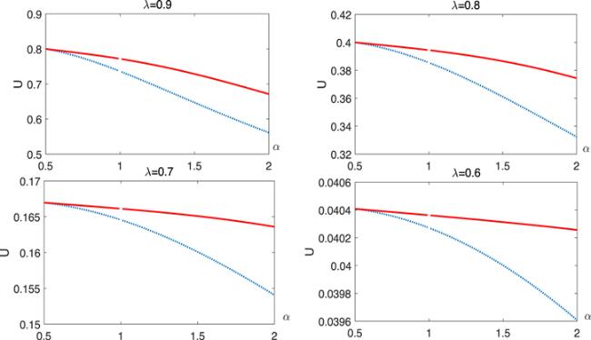
Figure 1. For $\alpha \in \left(\tfrac{1}{2},1\right)\cup (1,2]$, the comparison between lower and upper bounds, (a), (b), (c) and (d) represent, respectively, the cases of λ = 0.9, p = 0.8, p = 0.7 and p = 0.6.
In the case of $\alpha =\tfrac{1}{n+1}$, where n is a positive integer. For fixed λ = 0.9, 0.8, 0.7, 0.6, by comparing the upper and the lower bounds through figure 2, we find the following results.

We can find the differences between the upper and lower bounds increase with increase of the positive integer value n.

We can find the differences between the upper and lower bounds increase with increase of the maximum eigenvalue of the state ρ.

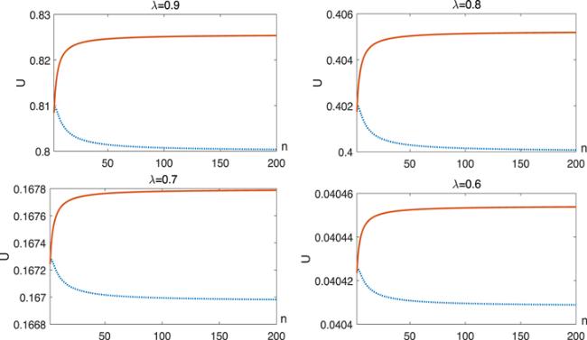
Figure 2. For $\alpha =\tfrac{1}{n+1}$, where n is a positive integer, the comparison between lower and upper bounds, (a), (b), (c) and (d) represent, respectively, the cases of λ = 0.9, λ = 0.8, λ = 0.7 and λ = 0.6.
In the following, we compare the tendency of ${ \mathcal U }(\rho )$ with respect to θ or φ for the different degree α. In figure 3, we plot ${ \mathcal U }(\rho )$ as functions of θ or φ for several values of α, one can find the tendency of ${ \mathcal U }(\rho )$ with respect to θ or φ are the same. The conclusions are opposite to uncertainty relations based on the Rényi entropy and Tsallis entropy. In fact, Alfredo Luis found that the minimum joint uncertainty states for some fluctuation measures are the maximum joint uncertainty states of other fluctuation measures, and vice versa [29].
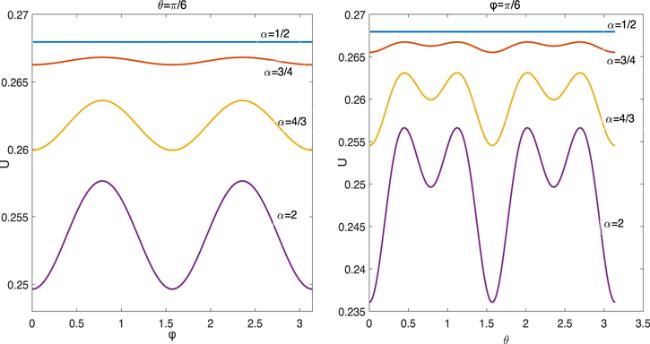
Figure 3. For the different degrees α, plots of ${ \mathcal U }(\rho )$ with respect to θ or φ.

5. Conclusion

In the paper, we researched the quantum uncertainty relations of quantum coherence based on three MUBs for the single qubit system. MUBs are eigenvector of Pauli matrices σx, σy, and σz. The coherence measure we studied is TREOC. The upper and lower bounds of sums of coherence were obtained for α ∈ [0, 1) ∪ (1, 2]. By considering the variations of upper and lower bounds with respect to α, the upper bound is equal to the lower bound for the special $\alpha =\tfrac{1}{2}$, and the differences between the upper and lower bounds will increase as α increases. We discussed the tendency of the sum of coherence, and find it is different from the uncertainty relations based on the Rényi entropy and Tsallis entropy [29].
There are many further issues need to be solved. For other coherence measures, we can discuss the quantum uncertainty relations of coherence. And for high-dimensional quantum systems, the quantum uncertainty relation of coherence is also an interesting subject for the future work.

This paper is supported by Startup Foundation for Doctors of Nanchang Hangkong University (No. EA201907210).

1
Scully M O Zubairy M S 1997 Quantum Optics Cambridge Cambridge University Press

2
Nielsen M A Chuang I L 2000 Quantum Computation and Quantum Information Cambridge Cambridge University Press

3
Berg J A 2014 Phys. Rev. Lett. 113 150402

DOI

4
Horodecki M Oppenheim J 2013 Nat. Commun. 4 2059

DOI

5
Baumgratz T Cramer M Plenio M B 2014 Phys. Rev. Lett. 113 140401

DOI

6
Streltsov A Singh U Dhar H S Bera M N Adesso G 2015 Phys. Rev. Lett. 115 020403

DOI

7
Napoli C Bromley T R Cianciaruso M Piani M Johnston N Adesso G 2016 Phys. Rev. Lett. 116 150502

DOI

8
Yu C S 2017 Phys. Rev. A 95 042337

DOI

9
Shao L H Xi Z Fan H Li Y 2015 Phys. Rev. A 91 042120

DOI

10
Rana S Parashar P Lewenstein M 2016 Phys. Rev. A 93 012110

DOI

11
Yuan X Zhou H Cao Z Ma X 2015 Phys. Rev. A 92 022124

DOI

12
Rastegin A E 2016 Phys. Rev. A 93 032136

DOI

13
Zhao H Q Yu C S 2017 Sci. Rep. 8 299

DOI

14
Winter A Yang D 2016 Phys. Rev. Lett. 116 120404

DOI

15
Zhu H Hayashi M Chen L 2018 Phys. Rev. A 97 022342

DOI

16
Chitambar E Gour G 2016 Phys. Rev. Lett. 117 030401

DOI

17
Streltsov A Adesso G M B 2017 Rev. Mod. Phys. 89 041003

DOI

18
Bu K Singh U S Fei M 2017 Phys. Rev. Lett. 119 150405

DOI

19
Xi Z Li Y Fan H 2015 Sci. Rep. 5 10922

DOI

20
Du S Bai Z Guo Y 2015 Phys. Rev. A 91 052120

DOI

21
Luo Y Li Y Hsieh M H 2019 Phys. Rev. A 99 042306

DOI

22
Hu M L Fan H 2017 Phys. Rev. A 95 052106

DOI

23
Heisenberg W 1927 Uber den anschaulichen, d. Inhalt, quantentheoretischen Kinematik und Mechanik Z. Phys. 43 172

DOI

24
Robertson H P 1929 Phys. Rev. 34 163

DOI

25
Deutsch D 1983 Phys. Rev. Lett. 50 631

DOI

26
Maassen H Uffink J B M 1988 Phys. Rev. Lett. 60 1103

DOI

27
Puchała Z Rudnicki Ł Życzkowski K 2013 J. Phys. A: Math. Theor. 46 272002

DOI

28
Rudnicki Ł Puchała Z Życzkowski K 2014 Phys. Rev. A 89 052115

DOI

29
Luis A 2011 Phys. Rev. A 84 034101

DOI

30
Rastegin A E 2013 Quantum Inf. Process. 12 2947 2963

DOI

31
Berta M Christandl M Colbeck R Renes J M Renner R 2010 Nat. Phys. 6 659 662

DOI

32
Kurzyk D Pawela Ł Puchała Z 2018 Quantum Inf. Process. 17 193

DOI

33
Yao C M 2014 Sci. China—Phys. Mech. Astron. 57 1703 1711

DOI

34
Ming F 2018 Quantum Inf. Process. 17 9

DOI

35
Ma Z H Chen Z H Fei S M 2017 Sci. China—Phys. Mech. Astron. 60 010321

DOI

36
Xiao Y 2019 Phys. Rev. A 100 032118

DOI

37
Puchała Z Rudnicki Ł Krawiec A Życzkowski K 2018 J. Phys. A: Math. Theor. 51 175306

DOI

38
Chen B Fei S M Long G L 2016 Quantum Inf. Process. 15 2639 2648

DOI

39
Singh U Pati A K Bera M N 2016 Mathematics 4 47

DOI

40
Yuan X Bai G Peng T 2017 Phys. Rev. A 96 032313

DOI

41
Cheng S Hall M J W 2015 Phys. Rev. A 92 042101

DOI

42
Zhang F G Li Y M 2018 Sci. China—Phys. Mech. Astron. 61 080312

DOI

43
Rastegin A E 2018 Frontiers Phys. 13 130304

DOI

44
Ng H Y N Berta M Wehner S 2012 Phys. Rev. A 86 042315

DOI

45
Cong S Feng X Y 2006 Proc. 2006 Academic Exchange on System Simulation Technology and its Application (in Chinese)

Outlines

/