


1. Introduction
Quantum key distribution (QKD) [1] enables two terminals Alice and Bob to establish a secure communication system in the presence of the eavesdropper Eve. Its security is based on the principles of quantum physics instead of the complexity of mathematical problems. In the past decades, many experimental QKD protocols have been proposed and implemented [2–21], which makes QKD become the most prospective implementation of quantum communication. Unfortunately, real-life single-photon sources will produce multiphoton pulses in a certain probability and suffer photon number splitting (PNS) [22] attacks inevitably. To counter PNS attacks, different protocols and methods have been proposed, and one of the most widely used methods is the decoy-state method [23–25].
In the decoy-state method, Alice will randomly prepare pulses into different intensities. Then it will select one of the produced pulses as the signal state and the others as decoy states. The multi-intensity decoy-state methods commonly make one intensity correspond to one signal state or decoy state, which inevitably introduces side-channel information leakage and modulation errors due to intensity modulation. As in [26, 27], some methods are able to change or distinguish the characters of different light intensities, such as time and waveform, which is conductive to eavesdroppers to identify the decoy states and signal states, and therefore undermine the security of a QKD system. The passive decoy state method [28, 29] can solve this problem skillfully, which usually uses a heralded single-photon source (HSPS) to generate different local detection events as decoy and signal states. Besides, HSPS is also helpful to decrease the effect of the dark count and raise the transmission distance of QKD [30, 31]. Meanwhile, in existing schemes, a novel passive decoy-state method is proposed to tightly estimate channel parameters and enhance the system performance [31]. It designs a specific local detection structure consisting of a beam splitter and two identical detectors. But in real-life implementation, it is difficult to unify the parameters of two local detectors, including detection efficiency and dark count rate. Therefore, it is necessary to estimate the performance of this passive decoy-state QKD scheme with mismatched local detectors.
In this paper, we will introduce the theoretical model of the passive decoy-state QKD scheme with mismatched local detectors. Besides, we consider the system performance in finite-size regime, calculating the key rate with statistical fluctuations. In numerical simulation, we show the effect of different transmission efficiencies and dark count rates for infinite case and finite case. Finally, we will summarize our simulation results and give conclusions.
2. Theoretical model
The passive decoy-state QKD scheme is presented as in [32], and the schematic diagram is shown in figure 1. In this system, a pump light focuses on a nonlinear crystal (NC) and generates the signal light (S) and the idler light (I) through a spontaneous parametric down-conversion (SPDC) process [33]. Then the idler light will be split into two parts by a beam splitter (BS) and sent to two different local detectors (D1, D2), respectively [34].
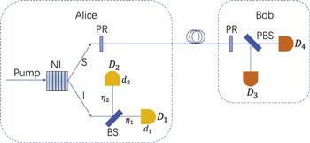
Figure 1. A schematic diagram of the passive decoy-state QKD [32]: NL, nonlinear crystal; BS, beam splitter; PR, polarization rotator; PBS, polarization beam splitter; D1 and D2, single-photon detectors. |
The clicking events of the two detectors can be divided into four events Xi(i = 1, 2, 3, 4). When an event Xi occurs, the signal state will be projected to the state ${\rho }_{l}={\sum }_{n}{a}_{n}^{l}| n\rangle \langle n| (l=x,y,z,w)$, where l is the state corresponding to the event Xi. The definitions of each event and corresponding probability are shown in table 1. As presented in [32], we can deduce the probability of each event:
$\begin{eqnarray}{a}_{n}^{l}=\sum _{m}{P}_{n,m}{P}_{{X}_{i}| {s}_{1}{s}_{2}}{P}_{{s}_{1}{s}_{2}| m}(l=x,y,z,w),\end{eqnarray}$
where Pn,m represents the joint probability that n photons in mode S and m photons in mode I. ${P}_{{X}_{i}| {s}_{1}{s}_{2}}$ is the conditional probability of the event Xi when the idler mode is projected to state ∣s1s2⟩. ${P}_{{s}_{1}{s}_{2}| m}$ denotes the conditional probability that an m-photon state is projected to state ∣s1s2⟩.Table 1. The definitions of each event and corresponding probability. |
| Event | D1 | D1 | State | Probability |
|---|---|---|---|---|
| X1 | 0 | 0 | x | axn |
| X2 | 1 | 0 | y | ayn |
| X3 | 0 | 1 | z | azn |
| X4 | 1 | 1 | w | awn |
When it is projected to the vacuum state, the local detector Di will click with a probability of di (the probability of the dark counts) or not click with a probability of (1 − di). The probabilities of the clicking event Xi in local detectors are shown in table 2.
Table 2. Conditional probability ${P}_{{X}_{i}| {s}_{1}{s}_{2}}$ that the event Xi when the idler light is projected to state ∣s1s2⟩. |
| Event | ${P}_{{X}_{1}| {s}_{1}{s}_{2}}$ | ${P}_{{X}_{2}| {s}_{1}{s}_{2}}$ | ${P}_{{X}_{3}| {s}_{1}{s}_{2}}$ | ${P}_{{X}_{4}| {s}_{1}{s}_{2}}$ |
|---|---|---|---|---|
| s1 = 0, s2 = 0 | (1 − d1)(1 − d2) | d1(1 − d2) | d2(1 − d1) | d1d2 |
| s1 ≠ 0, s2 = 0 | 0 | (1 − d2) | 0 | d2 |
| s1 = 0, s2 ≠ 0 | 0 | 0 | (1 − d1) | d1 |
| s1 ≠ 0, s2 ≠ 0 | 0 | 0 | 0 | 1 |
Considering the detection efficiency of Di (ηi) and the transmittance of local beam splitter (tv), the conditional probability ${P}_{{s}_{1}{s}_{2}| m}$ are given in table 3. Finally we can get the probability of x, y, z event (the probability of w state is negligible) in equation (1 ) with the Poisson distribution ${P}_{n}(\mu )={{\rm{e}}}^{-\mu }\tfrac{{\mu }^{n}}{n!}$:
$\begin{eqnarray}{a}_{n}^{x}={{\rm{e}}}^{-\mu }\displaystyle \frac{{\mu }^{n}}{n!}(1-{d}_{1})(1-{d}_{2}){\left[1-{\eta }_{2}+{t}_{v}({\eta }_{2}-{\eta }_{1})\right]}^{n},\end{eqnarray}$
$\begin{eqnarray}\begin{array}{l}{a}_{n}^{y}={{\rm{e}}}^{-\mu }\displaystyle \frac{{\mu }^{n}}{n!}\left\{(1-{d}_{2}){\left[1-(1-{t}_{v}){\eta }_{2}\right]}^{n}-(1-{d}_{1})\right.\\ \,\times \left.(1-{d}_{2}){\left[1-{\eta }_{2}+{t}_{v}({\eta }_{2}-{\eta }_{1})\right]}^{n}\right\},\end{array}\end{eqnarray}$
$\begin{eqnarray}\begin{array}{l}{a}_{n}^{z}={{\rm{e}}}^{-\mu }\displaystyle \frac{{\mu }^{n}}{n!}\left\{(1-{d}_{1}){\left(1-{t}_{v}{\eta }_{1}\right)}^{n}-(1-{d}_{1})\right.\\ \,\times \left.(1-{d}_{2}){\left[1-{\eta }_{2}+{t}_{v}({\eta }_{2}-{\eta }_{1})\right]}^{n}\right\}.\end{array}\end{eqnarray}$
Here ${t}_{v}\in [0,\tfrac{1}{2}]$, η1, η2 ∈ [0, 1] and d1, d2 ≪ 1. Therefore, for any n ≥ 2, $\begin{eqnarray}\begin{array}{l}\displaystyle \frac{{a}_{n}^{z}}{{a}_{n}^{x}}-\displaystyle \frac{{a}_{n-1}^{z}}{{a}_{n-1}^{x}}\\ =\,\displaystyle \frac{{\left(1-{t}_{v}{\eta }_{1}\right)}^{n}-(1-{d}_{2}){\left[1-{\eta }_{2}+{t}_{v}({\eta }_{2}-{\eta }_{1})\right]}^{n}}{(1-{d}_{2}){\left[1-{\eta }_{2}+{t}_{v}({\eta }_{2}-{\eta }_{1})\right]}^{n}}\\ -\,\displaystyle \frac{{\left(1-{t}_{v}{\eta }_{1}\right)}^{n-1}-(1-{d}_{2}){\left[1-{\eta }_{2}+{t}_{v}({\eta }_{2}-{\eta }_{1})\right]}^{n-1}}{(1-{d}_{2}){\left[1-{\eta }_{2}+{t}_{v}({\eta }_{2}-{\eta }_{1})\right]}^{n-1}}\\ =\,\displaystyle \frac{{\left(1-{t}_{v}{\eta }_{1}\right)}^{n-1}{\eta }_{2}(1-{t}_{v})}{(1-{d}_{2}){\left[1-{\eta }_{2}+{t}_{v}({\eta }_{2}-{\eta }_{1})\right]}^{n}}\geqslant 0.\end{array}\end{eqnarray}$
Similarly, we can get $\begin{eqnarray}\displaystyle \frac{{a}_{n}^{r}}{{a}_{n}^{l}}\geqslant \displaystyle \frac{{a}_{2}^{r}}{{a}_{2}^{l}}\geqslant \displaystyle \frac{{a}_{1}^{r}}{{a}_{1}^{l}},\end{eqnarray}$
where l, r ∈ {x, y, z} and l ≠ r. According to [35], given that these inequalities being respected by our passive source, the single-photon yield of our source can now be lower bounded.Table 3. Conditional probability ${P}_{{s}_{1}{s}_{2}| m}$ that an m-photon state is projected into state ∣s1s2⟩. |
| Case | ${P}_{{s}_{1}{s}_{2}| m}$ |
|---|---|
| s1 = 0, s2 = 0 | ${\left(1-{\eta }_{2}+{t}_{v}({\eta }_{2}-{\eta }_{1})\right)}^{m}$ |
| s1 ≠ 0, s2 = 0 | ${\left(1-(1-{t}_{v}){\eta }_{2}\right)}^{m}-{\left(1-{\eta }_{2}+{t}_{v}({\eta }_{2}-{\eta }_{1})\right)}^{m}$ |
| s1 = 0, s2 ≠ 0 | ${\left(1-{t}_{v}{\eta }_{1}\right)}^{m}-{\left(1-{\eta }_{2}+{t}_{v}({\eta }_{2}-{\eta }_{1})\right)}^{m}$ |
| s1 ≠ 0, s2 ≠ 0 | $1-{\left(1-{t}_{v}{\eta }_{1}\right)}^{m}-{\left(1-(1-{t}_{v}){\eta }_{2}\right)}^{m}+{\left(1-{\eta }_{2}+{t}_{v}({\eta }_{2}-{\eta }_{1})\right)}^{m}$ |
Denote Yi as the yield of the i-photon state, and Y0 as the background count rate including the dark count rate of Bob's detectors and channel background contributions. Using the linear channel model, Yi and error rate of i-photon state ei can be given by
$\begin{eqnarray}{Y}_{i}={Y}_{0}+{\eta }_{i}-{Y}_{0}{\eta }_{i},\end{eqnarray}$
$\begin{eqnarray}{e}_{i}=\displaystyle \frac{{e}_{0}{Y}_{0}+{e}_{d}{\eta }_{i}}{{Y}_{i}},\end{eqnarray}$
where ed represents the probability that a signal photon hit the erroneous detector, here ${\eta }_{i}=1-{\left(1-\eta \right)}^{i}$ is the transmittance of the i-photon state, where η = tABηBob denotes the total transmission and detection efficiency. It consists of the channel transmittance tAB = 10−αs/10 and the transmittance in Bobs side ηBob = tBobηD, where α and s represent the loss coefficient (dB km−1) and the length of the fiber (km), ηD is the detector efficiency at Bob's side.Based on the passive HSPS and channel model, the overall gain Ql and quantum bit error rate (QBER) El can be written as
$\begin{eqnarray}{Q}_{l}=\sum _{i=0}^{\infty }{Y}_{i}{a}_{i}^{l},\end{eqnarray}$
$\begin{eqnarray}{E}_{l}{Q}_{l}=\sum _{i=0}^{\infty }{e}_{i}{Y}_{i}{a}_{i}^{l}.\end{eqnarray}$
With the above formula and inequality (6 ), we can estimate the yield and error rate of single-photon pulses [35]:
$\begin{eqnarray}{Y}_{1}^{L}(l,r)=\displaystyle \frac{{a}_{2}^{r}{Q}_{l}-{a}_{2}^{l}{Q}_{r}-({a}_{2}^{r}{a}_{0}^{l}-{a}_{2}^{l}{a}_{0}^{r}){Y}_{0}^{U}}{{a}_{1}^{l}{a}_{2}^{r}-{a}_{1}^{r}{a}_{2}^{l}},\end{eqnarray}$
$\begin{eqnarray}{e}_{1}^{U}(l)=\displaystyle \frac{{E}_{l}{Q}_{l}-{e}_{0}{a}_{0}^{l}{Y}_{0}^{L}}{{a}_{1}^{l}{Y}_{1}^{L}},\end{eqnarray}$
where l, r ∈ {x, y, z} and l ≠ r. YL0 and YU0 represent the lower bound and upper bound of Y0, respectively. We can estimate them as [36] $\begin{eqnarray}{Y}_{0}^{L}=\max \left\{\displaystyle \frac{{a}_{1}^{y}{Q}_{x}-{a}_{1}^{x}{Q}_{y}}{{a}_{0}^{x}{a}_{1}^{y}-{a}_{0}^{y}{a}_{1}^{x}},\displaystyle \frac{{a}_{1}^{z}{Q}_{x}-{a}_{1}^{x}{Q}_{z}}{{a}_{0}^{x}{a}_{1}^{z}-{a}_{0}^{z}{a}_{1}^{x}},0\right\},\end{eqnarray}$
$\begin{eqnarray}{Y}_{0}^{U}=\min \left\{\displaystyle \frac{{E}_{x}{Q}_{x}}{{a}_{0}^{x}{e}_{0}},\displaystyle \frac{{E}_{y}{Q}_{y}}{{a}_{0}^{y}{e}_{0}},\displaystyle \frac{{E}_{z}{Q}_{z}}{{a}_{0}^{z}{e}_{0}}\right\}.\end{eqnarray}$
In the previous analysis, we just discussed the derivation of ${Y}_{1}^{L}(l,r)$, ${e}_{1}^{U}(l)$, YL0 and YU0 when the emitted pulses is infinite. But in real life, the number of pulses used for QKD systems is always finite. The finite pulses will inevitably lead to finite-size effect on the results when we analyze a QKD system quantitatively. Next, we will analyze the above variables with statistical fluctuations [32].
In BB84 protocol, we need to select two bases to code the signal light, namely X basis and Z basis. Denote PAX and PBX as the probability of choosing X basis in Alice's side and Bob's side, respectively. We can optimize two basis selection probability when we calculate secure key generation rate. If the total number of pulses we transmit is N0, then ${N}_{X}={N}_{0}{P}_{X}^{A}{P}_{X}^{B}$ and ${N}_{Z}={N}_{0}(1-{P}_{X}^{A})(1-{P}_{X}^{B})$ will be the number of pulses which can be successfully aligned to X and Z basis. Combined with analysis in [32], the counting rate Ql and overall error rate should satisfy11 ), (12 ) and (14 ) as
$\begin{eqnarray}N\hat{{Q}_{l}}={{NQ}}_{l}+{\delta }_{l},N\hat{{E}_{l}}\hat{{Q}_{l}}={{NE}}_{l}{Q}_{l}+{\delta }_{l}^{{\prime} },\end{eqnarray}$
where N = NX or NZ, δl ∈ [− Δl, Δl], ${{\rm{\Delta }}}_{l}=\gamma \sqrt{N\hat{{Q}_{l}}}$ and ${\delta }_{l}^{{\prime} }\in [-{{\rm{\Delta }}}_{l}^{{\prime} },{{\rm{\Delta }}}_{l}^{{\prime} }]$, ${{\rm{\Delta }}}_{l}=\gamma \sqrt{N\hat{{E}_{l}}\hat{{Q}_{l}}}$, here γ is a constant. Note that this standard Gaussian fluctuation method is based on the IID (independent and identical distribution) assumption. For the simplicity of calculation, we can change the equation as the following inequalities: $\begin{eqnarray}\hat{{Q}_{l}}(1-{{\rm{\Delta }}}_{1}^{l})\leqslant {Q}_{l}\leqslant \hat{{Q}_{l}}(1+{{\rm{\Delta }}}_{1}^{l}),\end{eqnarray}$
$\begin{eqnarray}\hat{{E}_{l}}\hat{{Q}_{l}}(1-{{\rm{\Delta }}}_{2}^{l})\leqslant {E}_{l}{Q}_{l}\leqslant \hat{{E}_{l}}\hat{{Q}_{l}}(1+{{\rm{\Delta }}}_{2}^{l}),\end{eqnarray}$
where ${{\rm{\Delta }}}_{1}^{l}=\gamma \sqrt{\tfrac{1}{\hat{{Q}_{l}}N}}$ and ${{\rm{\Delta }}}_{2}^{l}=\gamma \sqrt{\tfrac{1}{\hat{{E}_{l}}\hat{{Q}_{l}}N}}$. The above analysis can help us rewrite equations ( $\begin{eqnarray}{Y}_{1Z}^{L}(l,r)=\displaystyle \frac{{a}_{2}^{r}{Q}_{l}(1-{{\rm{\Delta }}}_{1Z}^{l})-{a}_{2}^{l}{Q}_{r}(1+{{\rm{\Delta }}}_{1Z}^{r})-({a}_{2}^{r}{a}_{0}^{l}-{a}_{2}^{l}{a}_{0}^{r}){Y}_{0}^{U}}{{a}_{1}^{l}{a}_{2}^{r}-{a}_{1}^{r}{a}_{2}^{l}},\end{eqnarray}$
$\begin{eqnarray}{e}_{1X}^{U}(l)=\displaystyle \frac{{Q}_{l}{E}_{l}(1+{{\rm{\Delta }}}_{2X}^{l})-{e}_{0}{a}_{0}^{l}{Y}_{0}^{L}}{{a}_{1}^{l}{Y}_{1X}^{L}},\end{eqnarray}$
where $\begin{eqnarray}\begin{array}{l}{Y}_{0}^{L}=\max \{\displaystyle \frac{{a}_{1}^{y}{Q}_{x}(1-{{\rm{\Delta }}}_{1Z}^{x})-{a}_{1}^{x}{Q}_{y}(1+{{\rm{\Delta }}}_{1Z}^{y})}{({a}_{0}^{x}{a}_{1}^{y}-{a}_{0}^{y}{a}_{1}^{x})},\\ \displaystyle \frac{{a}_{1}^{z}{Q}_{x}(1-{{\rm{\Delta }}}_{1Z}^{x})-{a}_{1}^{x}{Q}_{z}(1+{{\rm{\Delta }}}_{1Z}^{z})}{({a}_{0}^{x}{a}_{1}^{z}-{a}_{0}^{z}{a}_{1}^{x})},0\},\end{array}\end{eqnarray}$
$\begin{eqnarray}\begin{array}{l}{Y}_{0}^{U}=\min \left\{\displaystyle \frac{{E}_{x}{Q}_{x}(1+{{\rm{\Delta }}}_{2Z}^{x})}{{a}_{0}^{x}{e}_{0}},\displaystyle \frac{{E}_{y}{Q}_{y}(1+{{\rm{\Delta }}}_{2Z}^{y})}{{a}_{0}^{y}{e}_{0}},\right.\\ \left.\displaystyle \frac{{E}_{z}{Q}_{z}(1+{{\rm{\Delta }}}_{2Z}^{z})}{{a}_{0}^{z}{e}_{0}}\right\}.\end{array}\end{eqnarray}$
Otherwise, we can consider statistical fluctuations using other methods in [37, 38]. Consequently we can get the lower bound of ${Y}_{1Z}^{L}$ and the upper bound of ${e}_{1X}^{U}$ in finite cases: $\begin{eqnarray}{Y}_{1Z}^{L}=\max \{{Y}_{1Z}^{L}(x,y),{Y}_{1Z}^{L}(x,z),{Y}_{1Z}^{L}(y,z)\},\end{eqnarray}$
$\begin{eqnarray}{e}_{1X}^{U}=\min \{{e}_{1X}^{U}(x),{e}_{1X}^{U}(y),{e}_{1X}^{U}(z)\}.\end{eqnarray}$
With the above deduction, we can calculate the secure key generation rate Rl as
$\begin{eqnarray}\begin{array}{l}{R}_{l}\geqslant (1-{P}_{X}^{A})(1-{P}_{X}^{B})\\ \left\{{a}_{1}^{l}{Y}_{1Z}^{L}[1-H({e}_{1X}^{U})]-{{fQ}}_{l}{H}_{f}({E}_{l})\right\},\end{array}\end{eqnarray}$
where f is the error correction efficiency, $H(x)=-x{\mathrm{log}}_{2}(x)-(1-x){\mathrm{log}}_{2}(1-x)$ is the binary Shannon function. Finally we can calculate the secure key generation rate: $\begin{eqnarray}R={R}_{x}+{R}_{y}+{R}_{z}.\end{eqnarray}$
3. Numerical simulations
In this section, we will display the numerical simulations to discuss the effect of detection efficiency ηi and dark count rate di of local detector on system performance. Meanwhile, the key rate under infinite case and finite case will be discussed and compared. All simulations use the device parameters: tv = 0.25, ηD = 0.5, d0 = 6.02 × 10⁻⁶, e0 = 0.5, ed = 0.03, f = 1.16, N0 = 109 and γ = 5.3 corresponding to a failure probability 10−7 [32].
First, we fix the dark counting rate as d1 = d2 = 10−6 to discuss the effect of local detection efficiency. Figure 2 shows the trend of the key generation rate R with the increase of transmission distance under different detection efficiencies η2. Here η1 is set as 0.5. Obviously better detection efficiency will lead to higher key generation rate R at the same distance. This result is quite consistent with our objective cognition. And when considering the finite-size effect, key rate decays faster compared with the infinite case.
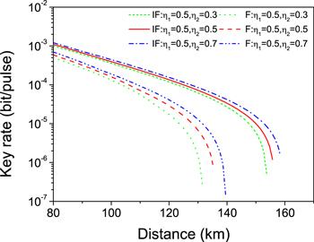
Figure 2. Relationship between security key generation rate R and transmission distance s for the infinite (IF) and finite case (F) (N0 = 109), where the detection efficiency of two local detectors ηi is divided into three groups: (1) η1 = 0.5, η2 = 0.3; (2) η1 = 0.5, η2 = 0.5; (3) η1 = 0.5, η2 = 0.7. |
Meanwhile, η1 and η2 can be jointly optimized to explore the effects on key rate in figure 3. As presented in the figure, increasing the value of η1 or η2 will improve R significantly. To be noted, if we fix the sum of η1 and η2, key rate will perform better when η2 is greater than η1 because the transmittance of local beam splitter tv is 0.25. As a result, the number of photons entering D1 will be more than entering D2. Consequently, the influence of η2 on the key generation rate R will be greater than η1.
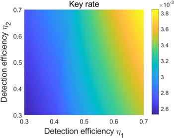
Figure 3. Joint optimization graph of η1 and η2 at a transmission distance of 50 km when the number of total pulses is finite. |
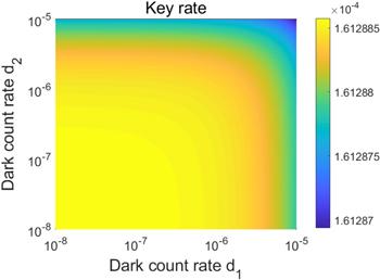
Accordingly, we can simulate the relationship between dark count rate d2 and the key generation rate R in figure 4. The curves corresponding to different cases in the figure are almost overlapped. Obviously, the dark count rate di of two detectors at Alice's side has little effect on the key generation rate R. Meanwhile, we display the joint effect of di in figure 5 as well. Increasing the values of d1 and d2 will only decrease the value of R on a small scale.
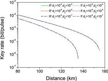
Figure 4. Relationship between security key generation rate R and transmission distance s for the infinite (IF) and finite case (F) (N0 = 109), where the dark count rate of two local detectors di is divided into three groups: (1) d1 = 106, d2 = 10−5; (2) d1 = 10−6, d2 = 10−6; (3) d1 = 10−6, d2 = 10−7. |
Figure 5. Joint effect on key rate of d1 and d2 at a transmission distance of 100 km when the number of total pulses is N0 = 109. |
4. Conclusions
In summary, we have studied the effect of local detection efficiency and dark count rate on the performance of passive decoy-state QKD when local detectors' parameters are asymmetric. Through mathematical analysis, we present the secure key generation rate R for both infinite-size and finite-size cases with the mismatched detector parameters. Based on the theoretical model, we display the relationship between key rate and two detectors' parameters. As a result, the detection efficiencies of local detectors affect the key generation rate more obviously than dark count rate. Therefore, our work will provide a reference value for a further research of passive decoy-state QKD systems with mismatched local detectors.
Otherwise, in this paper, we only discuss the case of two local mismatched detectors. But in realistic experiment, the parameters of detectors at Bob's side are often asymmetric as well, which will affect the solution of Yi and ei. Reference [39] has provided a linear channel loss model to explore the influence of detectors at Bob's side for the case of equal (or unequal) prepared basis and measurement basis. Combined with this model, we can extend our method to be more applicable to the real-life implementation.