


1. Introduction
To date, the Bohr Hamiltonian has been one of the most important phenomenological models for nuclear collective motion [1–4]. The Hamiltonian with various types of potential V(β, γ) has been adopted in describing spectra of nuclei in both transitional and well-deformed regions, of which the eigenvalue problem can either be solved numerically or analytically. Recently, there has been renewed interest in the collective model partly due to the critical point symmetries emerging at the critical point of the vibrational to γ-soft shape phase transition, called E(5) [5], and at that of the vibrational to axially deformed shape phase transition, called X(5) [6], which were derived from Bohr Hamiltonians with a β-part infinite well potential. In the E(5) case, the potential only depends on the β variable, which leads to the perfect separation of variables. In the X(5) case, nevertheless, it is unavoidable that β2 always appears in the γ-part of the eigen-equation when the intrinsic shape is assumed to be axially deformed with a non-trivial γ-part potential, for which a perfect variable separation may not be possible. In such a case, a numerical diagonalization procedure is required in order to get accurate wavefunctions of the system [7], of which the application to the X(5) case with analysis is detailed in [8, 9]. Very recently, the γ-unstable Bohr Hamiltonian with quasi-exactly solvable decatic potential and a centrifugal barrier is considered to describe nuclei near the critical point of the vibrational to γ-unstable (shape) phase transition [10], which shows that the decatic potential is better for description of even–even nuclei near the E(5) critical point.
In this work, we study the Bohr Hamiltonian with quasi-exactly solvable decatic β-part potential adopted in [10] to describe even–even nuclei in the vibrational to axially deformed transitional region.
The decatic model consists of a potential for the β-part of the Bohr Hamiltonian β collective variable from 2 up to 10. Here we consider a centrifugal term as well to obtain more accurate results. For simplicity, similar to the approximation made previously [6, 19–29], in which the $\left\langle {\beta }^{2}\right\rangle $ was treated as a free parameter, in this work, the $\left\langle {\beta }^{2}\right\rangle $ of each eigenstate is rigorously evaluated by using the corresponding β-part wavefunction. In section 2 , we present the Bohr Hamiltonian and the related analytical solutions concerned. The model is used to reproduce the energy ratios and B(E2) values of the X(5) model in the ground and beta band, of which the results are presented in section 3 . Applications of the model to describe some low-lying energy ratios and relevant B(E2) values of even–even X(5) candidates 150Nd, 156Dy, 164Yb, 168Hf, 174Yb, 176,178,180Os, 188,190Os, and even–even 154−158Gd within the X(5) critical point to the axially deformed region are shown in section 4 .
2. Bohr Hamiltonian and energy spectrum
The Bohr Hamiltonian is written in terms of the collective variables as [1–3]2.2 ) into (2.1 ), the total wavefunction can approximately be separated as $\Psi$(β, γ, ${\vartheta }_{i})\,=\xi (\beta )\eta (\gamma ){{ \mathcal D }}_{M,K}^{L}({\vartheta }_{i})$, where ϑi (i = 1, 2, 3) are the Euler angles, with which one gets two differential equations for the collective variables [6]:2.4 ) can be expressed explicitly as2.4 ) can be expressed as
$\begin{eqnarray}\begin{array}{l}H=-\displaystyle \frac{{{\hslash }}^{2}}{2B}\left[\displaystyle \frac{1}{{\beta }^{4}}\displaystyle \frac{\partial }{\partial \beta }{\beta }^{4}\displaystyle \frac{\partial }{\partial \beta }+\displaystyle \frac{1}{{\beta }^{2}\sin \left(3\gamma \right)}\displaystyle \frac{\partial }{\partial \gamma }\right.\\ \times \,\left.\sin \left(3\gamma \right)\displaystyle \frac{\partial }{\partial \gamma }-\displaystyle \frac{1}{4{\beta }^{2}}\displaystyle \sum _{k=1}^{3}\displaystyle \frac{{Q}_{k}^{2}}{{\sin }^{2}\left(\gamma -\tfrac{2}{3}\pi k\right)}\right]\\ +\,V(\beta ,\gamma ),\end{array}\end{eqnarray}$
where B is the mass parameter, β and γ are the usual collective coordinates describing the shape of the nuclear surface, and Qk (k = 1, 2, 3) stand for the operators of the total angular momentum projections in the intrinsic frame. For the axially deformed case, components of the moment of inertia involved in the rotational term can be approximately expanded in terms of γ around γ = 0 such that $\begin{eqnarray}\begin{array}{l}\sum _{k=1}^{3}\displaystyle \frac{{Q}_{k}^{2}}{{\sin }^{2}\left(\gamma -\tfrac{2\pi }{3}k\right)}\simeq \displaystyle \frac{4}{3}\left({Q}_{1}^{2}+{Q}_{2}^{2}+{Q}_{3}^{2}\right)\\ +{Q}_{3}^{2}\left(\displaystyle \frac{1}{{\sin }^{2}\gamma }-\displaystyle \frac{4}{3}\right).\end{array}\end{eqnarray}$
By substituting ( $\begin{eqnarray}\begin{array}{l}\left[-\displaystyle \frac{1}{{\beta }^{4}}\displaystyle \frac{\partial }{\partial \beta }{\beta }^{4}\displaystyle \frac{\partial }{\partial \beta }+\displaystyle \frac{1}{3{\beta }^{2}}L(L+1)+u(\beta )\right] \xi (\beta )={\varepsilon }_{\beta }\xi (\beta ),\end{array}\end{eqnarray}$
$\begin{eqnarray}\begin{array}{l}\left[-\displaystyle \frac{1}{\left\langle {\beta }^{2}\right\rangle \sin 3\gamma }\displaystyle \frac{\partial }{\partial \gamma }\sin 3\gamma \displaystyle \frac{\partial }{\partial \gamma }+\displaystyle \frac{1}{4\left\langle {\beta }^{2}\right\rangle }{K}^{2}\right.\\ \times \,\left.\left(\displaystyle \frac{1}{{\sin }^{2}\gamma }-\displaystyle \frac{4}{3}\right)+v(\gamma )\right]\eta (\gamma )={\varepsilon }_{\gamma }\eta (\gamma ),\end{array}\end{eqnarray}$
where $\tfrac{2{BE}}{{{\hslash }}^{2}}=\varepsilon ={\varepsilon }_{\beta }+{\varepsilon }_{\gamma }$ is the reduced energy, $\tfrac{2B}{{{\hslash }}^{2}}V(\beta ,\gamma )=u(\beta )+v(\gamma )$ is the reduced potential, and $\begin{eqnarray}\left\langle {\beta }^{2}\right\rangle =\int | \xi (\beta ){| }^{2}\,{\beta }^{6}\,{\rm{d}}\beta .\end{eqnarray}$
Similar to the X(5) case, small amplitude fluctuation of γ with the harmonic potential $v(\gamma )={\left(3{a}_{\gamma }/2\right)}^{2}{\gamma }^{2}$ is assumed, with which ( $\begin{eqnarray}\begin{array}{l}\frac{{{\rm{d}}}^{2}\eta (\gamma )}{{\rm{d}}{\gamma }^{2}}+\frac{1}{\gamma }\frac{{\rm{d}}\eta (\gamma )}{{\rm{d}}\gamma }+\left(-\frac{{\left(K/2\right)}^{2}}{{\gamma }^{2}}\right.\\ \left.-\left\langle {\beta }^{2}\right\rangle {\left(\frac{3{a}_{\gamma }}{2}\right)}^{2}{\gamma }^{2}+\lt{\beta }^{2}\gt{\tilde{\varepsilon }}_{\gamma }\right)\eta (\gamma )=0,\end{array}\end{eqnarray}$
where ${\tilde{\varepsilon }}_{\gamma }={\varepsilon }_{\gamma }+\tfrac{{\left(K/2\right)}^{2}}{\left\langle {\beta }^{2}\right\rangle }\tfrac{4}{3}$. Thus, the γ-part wavefunction η(γ) and ${\tilde{\varepsilon }}_{\gamma }$ should be given by $\begin{eqnarray}\begin{array}{l}{\eta }_{{n}_{\gamma },K}(\gamma )={C}_{{n}_{\gamma },K}\,{\gamma }^{| K/2| }\exp \left[-\displaystyle \frac{3{a}_{\gamma }}{2}\left\langle {\beta }^{2}\right\rangle \displaystyle \frac{{\gamma }^{2}}{2}\right]\\ \times {{\rm{L}}}_{n}^{| K/2| }\left(\displaystyle \frac{3{a}_{\gamma }}{2}\left\langle {\beta }^{2}\right\rangle {\gamma }^{2}\right),\end{array}\end{eqnarray}$
$\begin{eqnarray}{\tilde{\varepsilon }}_{\gamma }=\displaystyle \frac{3{a}_{\gamma }}{\sqrt{\left\langle {\beta }^{2}\right\rangle }}\left(1+\left|K/2\right|+2n\right),\end{eqnarray}$
where Ln stands for the Laguerre polynomial with n = 0, 1, 2... being the order of the polynomial, and the quantum number nγ is related to n by [30] $\begin{eqnarray}{n}_{\gamma }=2n+\left|K/2\right|,\end{eqnarray}$
so that the eigen-energy ϵγ in ( $\begin{eqnarray}{\varepsilon }_{\gamma }=\displaystyle \frac{3{a}_{\gamma }}{\sqrt{\left\langle {\beta }^{2}\right\rangle }}\left({n}_{\gamma }+1\right)-\displaystyle \frac{4}{3}\displaystyle \frac{{\left(K/2\right)}^{2}}{\left\langle {\beta }^{2}\right\rangle }.\end{eqnarray}$
Due to the axial symmetry of the system, the quantum number K ≥ 0 will be used to label the wavefunction in the following. Accordingly, the first band is the ground band with K = 0 and nγ = 0; the first gamma band is with K = 2 and nγ = 1; and so on.Furthermore, the β-part reduced potential u(β) is taken to be the decatic form [10, 31] with2.11 ) in (2.3 ) with $\xi (\beta )=\tfrac{{\rm{\Phi }}(\beta )}{{\beta }^{2}}$, we have2.12 ) becomes2.16 ) are given by2.17 ) that A3 < 0 is always satisfied as long as f > 0, with which the solution (2.15 ) satisfies the boundary condition ${\mathrm{lim}}_{x\to \infty }\phi (x)=0$. Since A0 ≥ 3/4, ξ(x) at x = 0 is finite if F(x) is a polynomial in x. In order to search for polynomial solutions, F(x) is initially written as the following power series form:2.16 ) leads to the following four-term recursion relation for gm:2.23 ) that finite polynomial solutions for F(x) exist if and only if the quasi-exact solvability constraints2.1 ) is given by
$\begin{eqnarray}u(\beta )=\displaystyle \frac{{\kappa }^{4}}{{\beta }^{2}}+a{\beta }^{2}+b{\beta }^{4}+c{\beta }^{6}+d{\beta }^{8}+f{\beta }^{10},\end{eqnarray}$
in which κ, a, b, c, d, f are real parameters. Using ( $\begin{eqnarray}\begin{array}{l}\frac{{{\rm{d}}}^{2}{\rm{\Phi }}(\beta )}{{\rm{d}}{\beta }^{2}}+\left({\varepsilon }_{\beta }-\frac{P}{{\beta }^{2}}-a{\beta }^{2}-b{\beta }^{4}\right.\\ \left.-c{\beta }^{6}-{d}{\beta }^{8}-f{\beta }^{10}\Space{0ex}{2.50ex}{0ex}\right){\rm{\Phi }}(\beta )=0,\end{array}\end{eqnarray}$
where $P=\tfrac{L(L+1)}{3}+{\kappa }^{4}+2$. Let $\begin{eqnarray}{\rm{\Phi }}(x)=\displaystyle \frac{\phi (x)}{\sqrt[4]{x}}\end{eqnarray}$
with x = β2. Equation ( $\begin{eqnarray}\begin{array}{l}\frac{{{\rm{d}}}^{2}\phi (x)}{{\rm{d}}{x}^{2}}+\left(\frac{\frac{\varepsilon \beta }{4}}{x}+\frac{\frac{3}{16}-\frac{P}{4}}{{x}^{2}}-\frac{a}{4}-\frac{b}{4}x\right.\\ \left.-\frac{c}{4}{x}^{2}-\frac{{d}}{4}{x}^{3}-\frac{f}{4}{x}^{4}\right)\phi (x)=0.\end{array}\end{eqnarray}$
Similar to the procedure shown in [10, 31], we use the following ansatz for φ(x): $\begin{eqnarray}\phi (x)={x}^{{A}_{0}}\exp \left[{A}_{1}x+{A}_{2}{x}^{2}+{A}_{3}{x}^{3}\right]F(x),\end{eqnarray}$
where F(x) is a polynomial in x, and Ai (i = 0, 1, 2, 3) are parameters to be determined, with which one gets the differential equation for the polynomial F(x): $\begin{eqnarray}\begin{array}{l}{xF}^{\prime\prime} (x)+\left({B}_{0}+{B}_{1}x+{B}_{2}{x}^{2}+{B}_{3}{x}^{3}\right)F^{\prime} (x)\\ +\left({C}_{0}+{C}_{1}x+{C}_{2}{x}^{2}\right)F(x)=0\end{array}\end{eqnarray}$
and solution of Ai: $\begin{eqnarray}{A}_{0}=\displaystyle \frac{1}{4}\left(2+\sqrt{1+4P}\right),\end{eqnarray}$
$\begin{eqnarray}{A}_{1}=\frac{{{d}}^{2}-4{cf}}{16{f}^{3/2}},\end{eqnarray}$
$\begin{eqnarray}{A}_{2}=\frac{-{d}}{8\sqrt{f}},\end{eqnarray}$
$\begin{eqnarray}{A}_{3}=\displaystyle \frac{-\sqrt{f}}{6},\end{eqnarray}$
while the parameters appearing in equation ( $\begin{eqnarray}\begin{array}{rcl}{B}_{0} & = & 2{A}_{0},\quad {B}_{1}=2{A}_{1},\quad {B}_{2}=4{A}_{2},\quad {B}_{3}=6{A}_{3},\\ {C}_{0} & = & \displaystyle \frac{{\varepsilon }_{\beta }}{4}+2{A}_{0}{A}_{1},\\ {C}_{1} & = & -\displaystyle \frac{a}{4}+{A}_{1}^{2}+2{A}_{2}+4{A}_{0}{A}_{2},\\ {C}_{2} & = & -\displaystyle \frac{b}{4}+4{A}_{1}{A}_{2}+6{A}_{3}+6{A}_{0}{A}_{3}.\end{array}\end{eqnarray}$
It can be observed from ( $\begin{eqnarray}F(x)=\sum _{m=0}^{\infty }{g}_{m}{x}^{m},\end{eqnarray}$
with which equation ( $\begin{eqnarray}\begin{array}{l}(m+1){B}_{0}\,{g}_{m+1}+({C}_{0}+m\,{B}_{1}){g}_{m}\\ +\left({C}_{1}+m(m+1)+(m-1){B}_{2}\right){g}_{m-1}\\ +({C}_{2}+(m-2){B}_{3}){g}_{m-2}=0.\end{array}\end{eqnarray}$
with the boundary condition gk = 0 for k ≤ −1. It can be easily proven by using ( $\begin{eqnarray}a={a}_{{m}_{\beta },L}=4\left({A}_{1}^{2}+2(2{m}_{\beta }+1){A}_{2}+4{A}_{0}{A}_{2}\right),\end{eqnarray}$
$\begin{eqnarray}b={b}_{{m}_{\beta },L}=8\left(2{A}_{1}{A}_{2}+3({m}_{\beta }+1){A}_{3}+3{A}_{0}{A}_{3}\right)\end{eqnarray}$
are satisfied, where mβ = 0, 1, 2, ⋯ , with which the polynomial $F(x)\equiv {F}_{{m}_{\beta }}(x)$ is a polynomial of order mβ with the reduced eigen-energy given by $\begin{eqnarray}{\varepsilon }_{\beta }=-8\left({m}_{\beta }+{A}_{0}\right){A}_{1}.\end{eqnarray}$
Finally, the total reduced eigen-energy of the Hamiltonian ( $\begin{eqnarray}\begin{array}{rcl}{\varepsilon }_{{m}_{\beta }\,{n}_{\gamma }\,L\,K} & = & -8\left({m}_{\beta }+{A}_{0}\right){A}_{1}\\ & & +\displaystyle \frac{3{a}_{\gamma }}{\sqrt{\left\langle {\beta }^{2}\right\rangle }}\left({n}_{\gamma }+1\right)-\displaystyle \frac{4}{3}\displaystyle \frac{{\left(K/2\right)}^{2}}{\left\langle {\beta }^{2}\right\rangle }.\end{array}\end{eqnarray}$
3. Comparison to the X(5) model
In this section, in order to show the similarity to and difference from the X(5) model, the model with quasi-exactly solvable decatic potential is used to fit the X(5) model results, aγ will be set to be zero for this case, of which the results with K = 0 are in accordance with the X(5) model results shown in [6].
The energy ratios defined by2.27 ) and (3.1 ), the energy ratio R becomes independent of the parameters c, d, and f of this model when aγ = 0 and K = 0. Hence, the only parameter κ is determined from the best fit to the X(5) model results RX(5). The fitting results of this model with those of the X(5) model are shown in table 1, in which only the K = 0 bands, namely the ground and the first beta band characterized by mβ = 0, 1 and L = 0+, 2+,..., respectively, are considered.
$\begin{eqnarray}\begin{array}{l}R({m}_{\beta },L)\\ =\displaystyle \frac{\varepsilon ({m}_{\beta },{n}_{\gamma }=0,L,K=0)-\varepsilon (0,0,0,0)}{\varepsilon (0,0,2,0)-\varepsilon (0,0,0,0).}\end{array}\end{eqnarray}$
shown in [6] are considered in our fitting. As shown in (Table 1. Low-lying level energy ratios R(mβ, L) = (ϵ(mβ, nγ = 0, L, K = 0) − ϵ(0, 0, 0, 0))/(ϵ(0, 0, 2, 0) − ϵ(0, 0, 0, 0)) related to the level energies of the ground band (mβ = 0) and the first β band (mβ = 1) near the X(5) critical point fitted by the model with the decatic model. It should be noted that only the parameter κ is involved in the energy ratios R(mβ, L) of the decatic case. |
| R(mβ, L) | X(5) | Decatic |
|---|---|---|
| 0g | 0.00 | 0.00 |
| 2g | 1.00 | 1.00 |
| 4g | 2.90 | 3.03 |
| 6g | 5.40 | 5.68 |
| 8g | 8.50 | 8.69 |
| 10g | 12.00 | 11.91 |
| 0β | 5.60 | 6.36 |
| 2β | 7.50 | 7.36 |
| 4β | 10.70 | 9.39 |
| χ2 | 0.30 | |
| κ = 1.62 | ||
| c = 159 | ||
| d = f = 1 |
The quadrupole operator can be written as3.2 ) is effective for intra-band transitions, while only the second term of (3.2 ) is effective for inter-band transitions. Accordingly, the B(E2) value, $B\left(E2;i\to f\right)$, can be expressed as
$\begin{eqnarray}\begin{array}{c}{T}_{\mu }^{(E2)}=t\,\beta \left(\Space{0ex}{2.5ex}{0ex}{{ \mathcal D }}_{\mu ,0}^{(2)}({\vartheta }_{i})\cos (\gamma )\right.\\ \left.+\frac{1}{\sqrt{2}}\left({{ \mathcal D }}_{\mu ,2}^{(2)}({\vartheta }_{i})+{{ \mathcal D }}_{\mu ,-2}^{(2)}({\vartheta }_{i})\right)\sin (\gamma )\right),\end{array}\end{eqnarray}$
where t is the effective charge. The O(3)-reduced matrix element of ${T}_{\mu }^{(E2)}$ is taken as $\begin{eqnarray}\begin{array}{c}\left\langle {L}_{f}{M}_{f}{K}_{f}\right|{T}_{\mu }^{\left({\rm{E}}2\right)}\left|{L}_{i}{M}_{i}{K}_{i}\right\rangle \\ =\ \frac{\left({L}_{i},{M}_{i};2,\mu | {L}_{f},{M}_{f}\right)}{\sqrt{2{L}_{f}+1}}\left\langle {L}_{f}{K}_{f}\right|\left|{T}^{\left({\rm{E}}2\right)}\right|\left|{L}_{i}{K}_{i}\right\rangle \end{array}\end{eqnarray}$
according to the Wigner–Eckart theorem. As mentioned in [6, 21], only the first term of ( $\begin{eqnarray}\begin{array}{ccl}B\left(E2;i\to f\right) & = & \frac{5}{16\pi }{t}^{2}\left({L}_{i},{K}_{i};2,{K}_{f}\right.\\ & & \,-\,{K}_{i}{\left|{L}_{f},{K}_{f}\right)}^{2}I{(i\to f)}^{2}G{(i\to f)}^{2},\end{array}\end{eqnarray}$
where the Clebsch–Gordan coefficient is denoted by $\left({L}_{i},{K}_{i};2,{K}_{f}-{K}_{i}\left|{L}_{f},{K}_{f}\right)\right.$ and $\begin{eqnarray}I(i\to f)=\int {\xi }_{i}(\beta )\,{\xi }_{f}(\beta )\,{\beta }^{5}\,\,{\rm{d}}\beta ,\end{eqnarray}$
$\begin{eqnarray}G(i\to f)=\int \sin (\gamma )\,{\eta }_{i}(\gamma )\,{\eta }_{f}(\gamma )\,\left|\sin (3\gamma )\right|\,\,{\rm{d}}\gamma .\end{eqnarray}$
In the fitting, the χ2 defined by $\begin{eqnarray}{\chi }^{2}=\displaystyle \frac{{\sum }_{i=1}^{N}{\left({R}_{i}^{\mathrm{Theor}}-{R}_{i}^{{\rm{X}}(5)}\right)}^{2}}{N-{N}^{* }}\end{eqnarray}$
is adopted, where ‘Theor' stands for this model or the quasi-exactly solvable sextic model, N is the number of total level energies or B(E2) values considered, and N* is the number of free parameters of the models involved in the fitting.With the fixed parameter κ determined by the energy ratios shown in table 1, the other three parameters c, d, and f of the decatic model are determined by the approximate orthogonality of the wavefunctions as described in [10] and the B(E2) values of the transitions satisfying the selection rule ΔK = 0. Specifically, the parameters d and f are fixed as d = f = 1, while c is adjusted in order to keep the approximate orthogonality of the wavefunctions, from which we get c = 159. Some related B(E2) values are shown in table 2, in which the X(5) model results are also provided.
Table 2. Some B(E2) ratios $R({\rm{E}}2;{L}_{i}\to {L}_{f})=B\left({\rm{E}}2;i\to f\right)/B\left({\rm{E}}2;{2}_{g}^{+}\to {0}_{g}^{+}\right)$ of the transitions within the ground and the first beta band and those of the inter-band transitions of the X(5) model fitted by the decatic model. For the decatic model, the best fit yields f = d = 1 and c = 159, with which the wavefunctions satisfy the orthogonality condition with respect to mβ approximately. |
| R(E2; Li → Lf) | X(5) | Decatic |
|---|---|---|
| 2g → 0g | 1.00 | 1.00 |
| 4g → 2g | 1.60 | 1.57 |
| 6g → 4g | 1.98 | 2.00 |
| 8g → 6g | 2.28 | 2.44 |
| 10g → 8g | 2.51 | 2.92 |
| 2β → 0β | 0.80 | 1.38 |
| 4β → 2β | 1.20 | 2.05 |
| 4β → 6g | 0.28 | 0.50 |
| 4β → 4g | 0.06 | 0.08 |
| 4β → 2g | 0.00 | 0.01 |
| 2β → 4g | 0.37 | 0.45 |
| 2β → 2g | 0.08 | 0.09 |
| 2β → 0g | 0.02 | 0.03 |
| 0β → 2g | 0.62 | 0.55 |
| χ2B(E2) | 0.13 |
4. Application to nuclei near the X(5) critical point
As shown in the previous section, the decatic model can provide results very close to those of the X(5) model. In this section, we intend to use the decatic model to describe both the nuclei near the X(5) critical point and those in the X(5) to rotational transition region, for which the first K = 2 gamma band is also considered. In this case, an additional free parameter related to the stiffness in the γ-part potential in all the models concerned is involved. Accordingly, the reduced energy of the X(5) model is now given by4.1 ) and (2.7 ), once $\left\langle {\beta }^{2}\right\rangle $ is evaluated, the parameter aγ should be adjusted not only to the gamma bandhead energy, but also to the B(E2) values considered, since aγ and $\left\langle {\beta }^{2}\right\rangle $ are also involved in the γ-part wavefunction as shown in (2.7 ).
$\begin{eqnarray}\begin{array}{ccl}{\varepsilon }_{X(5)} & = & {\left(\frac{{x}_{{m}_{\beta },\nu }}{{\beta }_{w}}\right)}^{2}+\frac{3{a}_{\gamma }}{\sqrt{\left\langle {\beta }^{2}\right\rangle }}\\ & & \times \ \left({n}_{\gamma }+1\right)-\frac{4}{3}\frac{{\left(K/2\right)}^{2}}{\left\langle {\beta }^{2}\right\rangle },\end{array}\end{eqnarray}$
where ${x}_{{m}_{\beta },\nu }$ denotes the (mβ + 1)-th zero of the Bessel function of order $\nu =\sqrt{\tfrac{L(L+1)}{3}+9/4}$, and two more free parameters aγ and βw, in which $\left\langle {\beta }^{2}\right\rangle $ of each eigenstate in all models concerned is rigorously evaluated. As clearly shown in (In order to show the fitting quality of the models, low-lying energy ratios and B(E2) ratios of some even–even X(5) candidate nuclei, such as 150Nd, 156Dy, 164Yb, 168Hf, 174Yb, 176,178,180Os, and 188,190Os, which, except for 164,174Yb, were considered as possible X(5) candidates studied in [29], are fitted by the decatic and the X(5) models. All experimental data are taken from [32]. Some predictions of the sextic model shown in [29] are also included for comparison. It is common in these nuclei that the bandhead energy of the first gamma band is higher than that of the first beta band. The energy ratios of these nuclei fitted by the two models considered here, the sextic model results [29], and the corresponding experimental values are shown in tables 3–5, in which the values of the corresponding model parameters after the fittings are provided in the lower part of the tables. The χ2 deviation of the fitting to the energy ratios for each nucleus by the X(5), decatic, and sextic [29] models is also provided. As shown in tables 3–5, the deviation of the energy ratios from the experimental values of these nuclei fitted in the X(5) model are larger than the other two models without exception, while the decatic model provides the best fitting results. Tables 6–8 provide B(E2) values of these even–even X(5) candidate nuclei normalized to B(E2; 2g → 0g) calculated from the X(5) and the decatic models with the corresponding model parameters shown in tables 3–5. In tables 6–8 the sextic model results provided in [29] are not included for comparison due to the fact that the higher-order term in the E2 transition operator introduced in [29] are not considered in the present calculation. In contrast to the energy ratios, it can be observed that the B(E2) values obtained from the X(5) model are better. The mean value of χ2 of both the energy ratios and the B(E2) values for all the even–even X(5) candidate nuclei fitted by the relevant models are shown in table 9. It is clearly shown that the decatic model provides better fitting results for the energy ratios, while the X(5) model is better at reproducing the B(E2) values of the even–even X(5) candidate nuclei concerned.
Table 3. Energy ratios defined in ( |
| 150Nd | 156Dy | 164Yb | 168Hf | ||||||||||||
|---|---|---|---|---|---|---|---|---|---|---|---|---|---|---|---|
| X(5) | Decatic | Sextic | Exp. | X(5) | Decatic | Sextic | Exp. | X(5) | Decatic | Exp. | X(5) | Decatic | Sextic | Exp. | |
| 0g | 0.00 | 0.00 | 0.00 | 0.00 | 0.00 | 0.00 | 0.00 | 0.00 | 0.00 | 0.00 | 0.00 | 0.00 | 0.00 | 0.00 | 0.00 |
| 2g | 1.00 | 1.00 | 1.00 | 1.00 | 1.00 | 1.00 | 1.00 | 1.00 | 1.00 | 1.00 | 1.00 | 1.00 | 1.00 | 1.00 | 1.00 |
| 4g | 3.06 | 3.08 | 3.14 | 2.93 | 3.06 | 3.01 | 2.98 | 2.93 | 3.14 | 3.18 | 3.13 | 3.14 | 3.16 | 3.25 | 3.11 |
| 6g | 5.92 | 5.85 | 6.15 | 5.53 | 5.92 | 5.61 | 5.69 | 5.59 | 6.18 | 6.28 | 6.16 | 6.18 | 6.20 | 6.57 | 6.10 |
| 8g | 9.47 | 9.02 | 9.89 | 8.68 | 9.47 | 8.55 | 8.97 | 8.82 | 9.98 | 10.04 | 9.92 | 9.98 | 9.84 | 10.85 | 9.78 |
| 10g | 13.63 | 12.45 | 14.23 | 12.28 | 13.63 | 11.68 | 12.73 | 12.52 | 14.46 | 14.26 | 14.22 | 14.46 | 13.90 | 15.95 | 13.99 |
| 12g | 18.37 | 16.04 | 19.08 | 16.27 | 19.59 | 18.81 | 18.89 | 19.59 | 18.24 | 21.80 | 18.58 | ||||
| 14g | 23.68 | 19.75 | 24.39 | 20.59 | 25.34 | 23.60 | 23.51 | 25.34 | 22.80 | 23.03 | |||||
| 2γ | 4.45 | 8.93 | 9.83 | 8.16 | 4.45 | 7.18 | 3.52 | 6.46 | 6.50 | 7.23 | 7.01 | 6.50 | 7.10 | 8.59 | 7.06 |
| 3γ | 5.28 | 9.49 | 10.78 | 9.22 | 5.28 | 7.78 | 5.37 | 7.42 | 7.30 | 8.10 | 8.14 | 7.30 | 7.93 | 9.65 | 8.31 |
| 4γ | 6.35 | 10.28 | 11.96 | 10.39 | 6.35 | 8.58 | 8.15 | 8.48 | 8.36 | 9.20 | 9.28 | 8.36 | 9.00 | 10.84 | 9.35 |
| 5γ | 7.62 | 9.55 | 11.56 | 9.69 | 9.67 | 10.53 | 10.93 | 9.67 | 10.27 | 12.35 | 11.17 | ||||
| 6γ | 9.09 | 10.66 | 11.07 | 11.19 | 11.72 | 14.17 | 12.50 | ||||||||
| 7γ | 10.73 | 11.88 | 12.55 | ||||||||||||
| 8γ | |||||||||||||||
| 0β | 6.94 | 5.19 | 5.68 | 5.19 | 6.94 | 4.71 | 7.08 | 4.90 | 7.62 | 8.30 | 8.13 | 7.59 | |||
| 2β | 9.01 | 6.51 | 7.41 | 6.53 | 9.01 | 6.02 | 7.95 | 6.01 | 9.82 | 9.37 | 9.62 | 8.53 | |||
| 4β | 12.76 | 9.01 | 10.43 | 8.74 | 12.76 | 8.40 | 9.07 | 7.90 | |||||||
| 6β | 17.50 | 12.10 | 14.32 | 11.83 | 17.50 | 11.27 | 10.22 | 10.43 | |||||||
| aγ | 1.00 | 13.00 | 1.00 | 11.00 | 1.00 | 6.00 | 1.00 | 9.00 | |||||||
| bw | 5.00 | 5.00 | 7.00 | 7.00 | |||||||||||
| κ | 1.15 | 0.99 | 1.99 | 1.88 | |||||||||||
| c | 39.00 | 37.00 | 17.00 | 35.00 | |||||||||||
| χ2 | 9.20 | 0.15 | 4.48 | 8.08 | 0.24 | 10.10 | 0.73 | 0.03 | 1.12 | 0.26 | 3.03 | ||||
Table 4. Same as table 3, but for 174Yb and 176,178Os. |
| 174Yb | 176Os | 178Os | |||||||||
|---|---|---|---|---|---|---|---|---|---|---|---|
| X(5) | Decatic | Exp. | X(5) | Decatic | Sextic | Exp. | X(5) | Decatic | Sextic | Exp. | |
| 0g | 0.00 | 0.00 | 0.00 | 0.00 | 0.00 | 0 | 0.00 | 0.00 | 0.00 | 0.00 | 0.00 |
| 2g | 1.00 | 1.00 | 1.00 | 1.00 | 1.00 | 1 | 1.00 | 1.00 | 1.00 | 1.00 | 1.00 |
| 4g | 3.80 | 3.30 | 3.31 | 3.10 | 3.02 | 3.02 | 2.93 | 3.10 | 3.02 | 2.98 | 3.02 |
| 6g | 8.26 | 6.80 | 6.88 | 6.05 | 5.65 | 5.78 | 5.50 | 6.05 | 5.65 | 5.68 | 5.76 |
| 8g | 14.11 | 11.40 | 11.64 | 9.71 | 8.62 | 9.14 | 8.57 | 9.71 | 8.62 | 8.95 | 9.03 |
| 10g | 21.19 | 16.97 | 17.47 | 14.03 | 11.79 | 12.99 | 12.10 | 14.03 | 11.81 | 12.67 | 12.72 |
| 12g | 29.39 | 23.38 | 24.34 | 18.96 | 15.10 | 17.26 | 16.05 | ||||
| 2γ | 22.97 | 21.54 | 21.37 | 5.43 | 7.48 | 7.54 | 6.39 | 5.43 | 7.48 | 7.20 | 6.54 |
| 3γ | 23.52 | 22.43 | 22.35 | 6.25 | 8.07 | 8.42 | 7.68 | 6.25 | 8.07 | 8.06 | 7.81 |
| 4γ | 24.59 | 23.61 | 23.61 | 7.31 | 8.86 | 9.56 | 9.06 | 7.31 | 8.87 | 9.19 | 9.18 |
| 5γ | 26.15 | 25.06 | 25.19 | 8.60 | 9.83 | 10.76 | 10.43 | 8.60 | 9.84 | 10.35 | 10.71 |
| 0β | 13.07 | 19.29 | 19.45 | 7.27 | 4.74 | 3.98 | 4.45 | 7.27 | 4.76 | 3.97 | 4.92 |
| 2β | 16.38 | 20.33 | 20.41 | 9.40 | 6.07 | 5.78 | 5.50 | 9.40 | 6.08 | 5.62 | 5.83 |
| 4β | 22.52 | 22.70 | 22.43 | 13.27 | 8.49 | 8.40 | 7.74 | ||||
| aγ | 1.00 | 19.00 | 1.00 | 11.00 | 1.00 | 11.00 | |||||
| bw | 16.00 | 6.00 | 6.00 | ||||||||
| κ | 3.00 | 0.99 | 1.00 | ||||||||
| c | 38.00 | 35.00 | 35.00 | ||||||||
| χ2 | 9.20 | 0.13 | 4.22 | 0.32 | 0.64 | 5.70 | 0.35 | 0.30 | |||
Table 5. Same as table 3, but for 180,188,190Os. |
| 180Os | 188Os | 190Os | ||||||||||
|---|---|---|---|---|---|---|---|---|---|---|---|---|
| X(5) | Decatic | Sextic | Exp. | X(5) | Decatic | Sextic | Exp. | X(5) | Decatic | Sextic | Exp. | |
| 0g | 0.00 | 0.00 | 0.00 | 0.00 | 0.00 | 0.00 | 0.00 | 0.00 | 0.00 | 0.00 | 0.00 | 0.00 |
| 2g | 1.00 | 1.00 | 1.00 | 1.00 | 1.00 | 1.00 | 1.00 | 1.00 | 1.00 | 1.00 | 1.00 | 1.00 |
| 4g | 3.14 | 3.05 | 3.07 | 3.09 | 3.06 | 3.15 | 3.13 | 3.08 | 2.99 | 2.94 | 3.09 | 2.93 |
| 6g | 6.18 | 5.76 | 5.98 | 6.02 | 5.92 | 6.14 | 6.15 | 6.07 | 5.70 | 5.41 | 6.01 | 5.63 |
| 8g | 9.98 | 8.85 | 9.57 | 9.52 | 9.47 | 9.70 | 9.88 | 9.77 | 9.03 | 8.15 | 9.61 | 8.93 |
| 10g | 14.46 | 12.18 | 13.73 | 13.38 | 13.63 | 13.65 | 14.17 | 14.00 | 12.92 | 11.05 | 13.76 | 12.62 |
| 12g | 18.37 | 17.86 | 18.93 | 18.42 | ||||||||
| 14g | 23.68 | 22.26 | 22.98 | |||||||||
| 2γ | 6.50 | 7.94 | 7.88 | 6.59 | 4.45 | 3.98 | 4.22 | 4.08 | 2.71 | 4.05 | 3.45 | 2.99 |
| 3γ | 7.30 | 8.55 | 8.80 | 7.74 | 5.28 | 4.88 | 5.20 | 5.10 | 3.57 | 4.83 | 4.38 | 4.05 |
| 4γ | 8.36 | 9.38 | 9.96 | 9.06 | 6.35 | 6.02 | 6.38 | 6.23 | 4.63 | 5.78 | 5.55 | 5.12 |
| 5γ | 9.67 | 10.38 | 11.22 | 10.64 | 7.62 | 7.36 | 7.71 | 7.62 | 5.88 | 6.86 | 6.81 | 6.45 |
| 6γ | 11.19 | 11.53 | 12.87 | 12.32 | 9.09 | 8.87 | 9.43 | 9.19 | 7.29 | 8.04 | 8.48 | 7.90 |
| 7γ | 10.73 | 10.53 | 11.01 | 10.87 | ||||||||
| 8γ | 12.53 | 12.30 | 12.87 | |||||||||
| 0β | 7.62 | 5.22 | 4.44 | 5.57 | 6.94 | 8.26 | 6.99 | 7.00 | 6.37 | 5.23 | 5.00 | 4.88 |
| 2β | 9.82 | 6.50 | 6.19 | 6.29 | 9.01 | 9.30 | 8.75 | 8.42 | 8.32 | 6.38 | 6.79 | 5.97 |
| 4β | 13.83 | 8.91 | 9.10 | 7.97 | ||||||||
| aγ | 1.00 | 11.00 | 1.00 | 5.00 | 1.00 | 4.00 | ||||||
| bw | 7.00 | 5.00 | 3.00 | |||||||||
| κ | 1.19 | 1.90 | 1.23 | |||||||||
| c | 33.00 | 34.00 | 14.00 | |||||||||
| χ2 | 4.62 | 0.57 | 0.76 | 0.10 | 0.29 | 0.05 | 0.82 | 0.58 | 0.47 | |||
Table 6. B(E2) values of the even–even X(5) candidate nuclei normalized to B(E2; 2g → 0g) calculated from the X(5), the decatic models with parameters the same as those shown in tables 3–5. The corresponding ${\chi }_{B(E2)}^{2}$ value is also provided according to the experimentally measured values. |
| 150Nd | 156Dy | 164Yb | |||||||
|---|---|---|---|---|---|---|---|---|---|
| X(5) | Decatic | Exp. | X(5) | Decatic | Exp. | X(5) | Decatic | Exp. | |
| 2g → 0g | 1.00 | 1.00 | 1.00 | 1.00 | 1.00 | 1.00 | 1.00 | 1.00 | 1.00 |
| 4g → 2g | 1.55 | 1.56 | 1.56 | 1.55 | 1.59 | 1.63 | 1.54 | 1.48 | 1.60 |
| 6g → 4g | 1.86 | 1.96 | 1.80 | 1.86 | 2.03 | 1.76 | 1.84 | 1.71 | 1.70 |
| 8g → 6g | 2.08 | 2.33 | 1.86 | 2.08 | 2.44 | 1.87 | 2.05 | 1.91 | 1.98 |
| 10g → 8g | 2.24 | 2.68 | 1.83 | 2.24 | 2.82 | 2.07 | 2.20 | 2.09 | 1.85 |
| 2β → 0β | 0.82 | 1.21 | 1.38 | 0.82 | 1.23 | 0.82 | 0.97 | ||
| 4β → 2β | 1.22 | 1.74 | 1.86 | 1.22 | 1.77 | 1.22 | 1.37 | ||
| 4β → 6g | 0.27 | 0.54 | 0.08 | 0.27 | 0.59 | 0.08 | 0.27 | 0.00 | |
| 4β → 4g | 0.06 | 0.07 | 0.06 | 0.07 | 0.09 | 0.06 | 0.02 | ||
| 4β → 2g | 0.00 | 0.00 | 0.00 | 0.00 | 0.00 | 0.00 | 0.00 | 0.06 | |
| 2β → 4g | 0.36 | 0.57 | 0.16 | 0.36 | 0.64 | 0.36 | 0.00 | ||
| 2β → 2g | 0.08 | 0.09 | 0.09 | 0.08 | 0.09 | 0.08 | 0.00 | ||
| 2β → 0g | 0.02 | 0.02 | 0.00 | 0.02 | 0.01 | 0.02 | 0.01 | ||
| 0β → 2g | 0.63 | 0.73 | 0.37 | 0.63 | 0.83 | 0.63 | 0.00 | ||
| 4γ → 2γ | 1.33 | 1.40 | 1.20 | 1.33 | 1.41 | 1.36 | 1.31 | ||
| 4γ → 2g | 0.81 | 0.85 | 0.00 | 0.81 | 0.86 | 0.81 | 0.78 | ||
| 3γ → 4g | 0.98 | 1.02 | 0.98 | 1.05 | 0.98 | 0.93 | |||
| 3γ → 2g | 2.39 | 2.49 | 2.39 | 2.53 | 2.40 | 2.29 | |||
| 2γ → 4g | 0.09 | 0.09 | 0.01 | 0.09 | 0.09 | 0.08 | 0.09 | 0.09 | |
| 2γ → 2g | 1.85 | 1.90 | 1.85 | 1.92 | 0.06 | 1.86 | 1.80 | ||
| 2γ → 0g | 1.25 | 1.28 | 0.03 | 1.25 | 1.28 | 0.05 | 1.26 | 1.25 | |
| ${\chi }_{{\rm{B}}({\rm{E}}2)}^{2}$ | 0.22 | 0.28 | 0.53 | 0.77 | 0.05 | 0.04 | |||
Table 7. Same as table 6, but for 168Hf, 174Hf, and 176Os. |
| 168Hf | 174Yb | 176Os | |||||||
|---|---|---|---|---|---|---|---|---|---|
| X(5) | Decatic | Exp. | X(5) | Decatic | Exp. | X(5) | Decatic | Exp. | |
| 2g → 0g | 1.00 | 1.00 | 1.00 | 1.00 | 1.00 | 1.00 | 1.00 | 1.00 | |
| 4g → 2g | 1.54 | 1.49 | 1.58 | 1.53 | 1.44 | 1.39 | 1.54 | 1.59 | |
| 6g → 4g | 1.84 | 1.75 | 1.85 | 1.81 | 1.61 | 1.84 | 1.84 | 2.03 | |
| 8g → 6g | 2.05 | 1.97 | 2.27 | 2.00 | 1.72 | 1.93 | 2.06 | 2.43 | |
| 10g → 8g | 2.20 | 2.19 | 2.40 | 2.15 | 1.81 | 1.67 | 2.22 | 2.81 | |
| 2β → 0β | 0.82 | 1.13 | 0.83 | 1.01 | 0.82 | 1.23 | |||
| 4β → 2β | 1.22 | 1.62 | 1.22 | 1.45 | 1.22 | 1.76 | |||
| 2β → 2g | 0.08 | 0.04 | 0.08 | 0.00 | 0.08 | 0.09 | |||
| 2β → 0g | 0.02 | 0.01 | 0.02 | 0.00 | 0.02 | 0.01 | |||
| 0β → 2g | 0.63 | 0.28 | 0.63 | 0.02 | 0.63 | 0.83 | |||
| 4γ → 4g | 2.50 | 2.38 | 2.50 | 2.25 | 2.50 | 2.78 | |||
| 4γ → 2g | 0.81 | 0.79 | 0.82 | 0.76 | 0.81 | 0.86 | |||
| 3γ → 4g | 0.98 | 0.94 | 0.98 | 0.91 | 0.98 | 1.05 | |||
| 3γ → 2g | 2.40 | 2.32 | 2.42 | 2.27 | 2.40 | 2.53 | |||
| 2γ → 4g | 0.09 | 0.09 | 0.09 | 0.09 | 0.09 | 0.09 | |||
| 2γ → 2g | 1.86 | 1.81 | 1.88 | 1.81 | 0.01 | 1.86 | 1.92 | ||
| 2γ → 0g | 1.26 | 1.26 | 1.29 | 1.27 | 1.26 | 1.28 | |||
| 4γ → 4β | 0.10 | 0.06 | 0.10 | 0.00 | 0.10 | 0.11 | |||
| 4γ → 2β | 0.11 | 0.06 | 0.11 | 0.00 | 0.11 | 0.17 | |||
| 3γ → 4β | 0.02 | 0.00 | 0.02 | 0.00 | 0.02 | 0.00 | |||
| 3γ → 2β | 0.22 | 0.11 | 0.22 | 0.00 | 0.22 | 0.28 | |||
| 2γ → 4β | 0.00 | 0.00 | 0.00 | 0.00 | 0.00 | 0.00 | |||
| 2γ → 2β | 0.11 | 0.05 | 0.11 | 0.00 | 0.10 | 0.10 | |||
| 2γ → 0β | 0.16 | 0.07 | 0.17 | 0.00 | 0.16 | 0.19 | |||
| ${\chi }_{{\rm{B}}({\rm{E}}2)}^{2}$ | 0.03 | 0.08 | 0.94 | 1.12 | |||||
Table 8. Same as table 6, but for 178,180,188,190Os. |
| 178Os | 180Os | 188Os | 190Os | |||||||||
|---|---|---|---|---|---|---|---|---|---|---|---|---|
| X(5) | Decatic | Exp. | X(5) | Decatic | Exp. | X(5) | Decatic | Exp. | X(5) | Decatic | Exp. | |
| 2g → 0g | 1.00 | 1.00 | 1.00 | 1.00 | 1.00 | 1.00 | 1.00 | 1.00 | 1.00 | 1.00 | 1.00 | 1.00 |
| 4g → 2g | 1.54 | 1.59 | 1.54 | 1.56 | 1.36 | 1.55 | 1.49 | 1.72 | 1.56 | 1.57 | 1.46 | |
| 6g → 4g | 1.84 | 2.03 | 1.84 | 1.96 | 1.13 | 1.86 | 1.77 | 1.78 | 1.89 | 1.97 | 1.57 | |
| 8g → 6g | 2.06 | 2.43 | 2.05 | 2.32 | 0.45 | 2.08 | 2.01 | 1.87 | 2.13 | 2.33 | 1.91 | |
| 10g → 8g | 2.22 | 2.80 | 2.20 | 2.66 | 2.24 | 2.25 | 2.31 | 2.66 | 1.67 | |||
| 0β → 2g | 0.63 | 0.82 | 0.63 | 0.68 | 0.63 | 0.27 | 0.01 | 0.63 | 0.22 | 0.03 | ||
| 6γ → 4γ | 2.90 | 3.24 | 2.50 | 3.14 | 2.87 | 2.69 | 0.94 | 2.78 | 3.01 | 0.90 | ||
| 5γ → 4γ | 2.35 | 2.65 | 0.81 | 2.56 | 2.32 | 2.17 | 2.24 | 2.45 | ||||
| 5γ → 3γ | 2.26 | 2.44 | 0.98 | 2.38 | 2.24 | 2.10 | 2.15 | 2.28 | ||||
| 4γ → 3γ | 3.14 | 3.42 | 2.40 | 3.33 | 3.10 | 2.91 | 2.98 | 3.17 | 0.90 | |||
| 4γ → 2γ | 1.35 | 1.41 | 0.09 | 1.39 | 1.33 | 1.26 | 0.61 | 1.27 | 1.33 | 0.74 | ||
| 6γ → 6g | 2.78 | 3.32 | 2.78 | 3.17 | 2.79 | 2.68 | 2.81 | 3.12 | 0.43 | |||
| 6γ → 4g | 0.72 | 0.82 | 0.72 | 0.79 | 0.72 | 0.69 | 0.00 | 0.72 | 0.77 | |||
| 5γ → 6g | 1.35 | 1.55 | 1.35 | 1.49 | 1.36 | 1.29 | 1.37 | 1.47 | ||||
| 5γ → 4g | 2.32 | 2.63 | 2.33 | 2.53 | 2.32 | 2.20 | 2.32 | 2.48 | ||||
| 4γ → 6g | 0.22 | 0.23 | 0.22 | 0.23 | 0.22 | 0.21 | 0.19 | 0.22 | 0.23 | |||
| 4γ → 4g | 2.50 | 2.77 | 2.50 | 2.68 | 2.50 | 2.37 | 2.50 | 2.63 | 0.42 | |||
| 4γ → 2g | 0.81 | 0.86 | 0.81 | 0.84 | 0.81 | 0.77 | 0.02 | 0.80 | 0.82 | 0.00 | ||
| 3γ → 4g | 0.98 | 1.05 | 0.98 | 1.02 | 0.98 | 0.93 | 0.98 | 1.01 | ||||
| 3γ → 2g | 2.40 | 2.53 | 2.40 | 2.48 | 2.39 | 2.28 | 2.36 | 2.42 | ||||
| 2γ → 4g | 0.09 | 0.09 | 0.09 | 0.09 | 0.09 | 0.09 | 0.09 | 0.09 | ||||
| 2γ → 2g | 1.86 | 1.92 | 1.86 | 1.89 | 1.85 | 1.79 | 0.21 | 1.83 | 1.86 | 0.46 | ||
| 2γ → 0g | 1.26 | 1.28 | 1.26 | 1.28 | 1.25 | 1.23 | 0.06 | 1.23 | 1.25 | 0.08 | ||
| ${\chi }_{{\rm{B}}({\rm{E}}2)}^{2}$ | 1.55 | 4.23 | 1.00 | 0.95 | 1.91 | 2.49 | ||||||
Table 9. Mean value of χ2 of the energy ratios and that of B(E2) values, ${\overline{{\chi }^{2}}}_{{\rm{B}}({\rm{E}}2)}$, of each model. |
| X(5) | Decatic | Sextic | |
|---|---|---|---|
| $\overline{{\chi }^{2}}\,\,\,\,\,$ | 4.38 | 0.29 | 2.48 |
| ${\overline{{\chi }^{2}}}_{{\rm{B}}({\rm{E}}2)}$ | 0.78 | 1.24 | — |
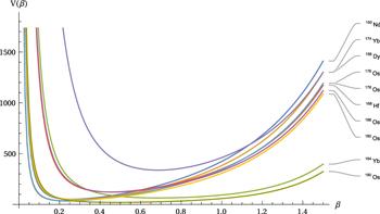
It would be interesting to depict the ground state potential of isotopes discussed here, after the determination of appropriate numerical values of potential constants. In figure 1, the decatic potential is depicted using the parameters mentioned in tables 3–5 for each isotope. The potential of each isotope is distinguished by color and its name. It is seen that there is a minimum for each isotope after which it increases rapidly.
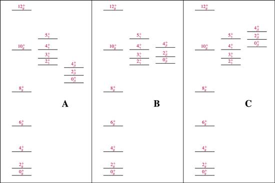
In fact, there are three different level patterns of nuclei near the X(5) critical point and those in between the X(5) critical point and the axially deformed shape as illustrated in figure 2, in which the relative positions of the beta and qgamma bandhead are different. Specifically, the beta-bandhead energy is lower than that of the gamma band in pattern A. The level pattern of the even–even X(5) candidate nuclei fitted above are of the A type, of which the B(E2) values can be well reproduced by the X(5) model, though the fitting quality of the X(5) model to the level energies is not good. The bandhead energies of the beta and gamma band are somehow (more or less) equal in pattern B, while the beta-bandhead energy is higher than that of the gamma band in pattern C. As shown in table 1 of [21], many deformed nuclei with level pattern C can be well described by the exactly separable reduced potential with $\tfrac{2B}{{{\hslash }}^{2}}V(\beta ,\gamma )=u(\beta )+v(\gamma )/{\beta }^{2}$, which, however, is not considered here. Most importantly, it is observed that the decatic model is the better at describing both the low-lying level energies and related B(E2) values of nuclei with level pattern B, which are also within the X(5) critical point to the axially deformed region.
Figure 2. Three possible level patterns classified according to the relative position of the beta- and gamma-bandhead energy of nuclei within the X(5) critical point to the axially deformed region. |
There are many deformed nuclei with level pattern B. Here we select even–even 154−158Gd as typical examples. Some low-lying energy ratios and relevant B(E2) values fitted by the X(5) and the decatic models described above are shown in tables 10 and 11, respectively, in which the experimental data are also taken from [32]. It can be observed from tables 10 and 11 and the mean value of χ2 of the energy ratios and B(E2) values for even–even 154−158Gd shown in table 12 that the decatic model in this case provides a better fitting quality to these nuclei with level pattern B.
Table 10. Energy ratios defined in ( |
| 154Gd | 156Gd | 158Gd | |||||||
|---|---|---|---|---|---|---|---|---|---|
| X(5) | Decatic | Exp. | X(5) | Decatic | Exp. | X(5) | Decatic | Exp. | |
| 0g | 0.00 | 0.00 | 0.00 | 0.00 | 0.00 | 0.00 | 0.00 | 0.00 | 0.00 |
| 2g | 1.00 | 1.00 | 1.00 | 1.00 | 1.00 | 1.00 | 1.00 | 1.00 | 1.00 |
| 4g | 3.17 | 3.10 | 3.01 | 3.40 | 3.25 | 3.24 | 3.50 | 3.28 | 3.29 |
| 6g | 6.27 | 5.94 | 5.83 | 7.01 | 6.58 | 6.57 | 7.32 | 6.71 | 6.78 |
| 8g | 10.15 | 9.24 | 9.30 | 11.63 | 10.79 | 10.85 | 12.24 | 11.15 | 11.37 |
| 10g | 14.74 | 12.85 | 13.30 | 17.14 | 15.70 | 15.92 | 18.15 | 16.43 | 16.97 |
| 12g | 20.00 | 16.65 | 17.75 | 23.50 | 21.15 | 21.63 | 24.97 | 22.41 | 23.45 |
| 2γ | 7.18 | 8.89 | 8.09 | 13.07 | 13.45 | 12.97 | 15.53 | 15.05 | 14.93 |
| 3γ | 7.97 | 9.56 | 9.16 | 13.77 | 14.31 | 14.03 | 16.19 | 15.95 | 15.92 |
| 4γ | 9.04 | 10.44 | 10.27 | 14.84 | 15.44 | 15.23 | 17.26 | 17.13 | 17.08 |
| 5γ | 10.35 | 11.51 | 11.64 | 16.24 | 16.82 | 16.94 | 18.71 | 18.58 | 18.63 |
| 6γ | 11.90 | 12.74 | 13.05 | 17.96 | 18.43 | 18.47 | 20.49 | 20.29 | 20.42 |
| 7γ | 13.65 | 14.11 | 14.71 | 19.96 | 20.26 | 20.79 | |||
| 8γ | 22.22 | 22.27 | 22.61 | ||||||
| 0β | 7.85 | 5.65 | 5.53 | 9.79 | 11.68 | 11.80 | 10.61 | 14.85 | 15.04 |
| 2β | 10.10 | 6.87 | 6.63 | 12.44 | 12.73 | 12.69 | 13.42 | 15.88 | 15.84 |
| 4β | 14.20 | 9.29 | 8.51 | 17.30 | 15.09 | 14.59 | 18.60 | 18.24 | 17.69 |
| aγ | 0.40 | 9.00 | 0.90 | 9.00 | 1.00 | 10.00 | |||
| βw | 19.00 | 13.00 | 13.00 | ||||||
| κ | 1.44 | 2.38 | 2.71 | ||||||
| c | 20.00 | 16.00 | 19.00 | ||||||
| χ2 | 4.69 | 0.26 | 1.27 | 0.09 | 2.43 | 0.15 | |||
Table 11. B(E2) values of even–even 154−158 Gd nuclei normalized to B(E2; 2g → 0g) calculated from the X(5), the decatic, and the sextic models with parameters the same as those shown in table 10. The corresponding ${\chi }_{B({\rm{E}}2)}^{2}$ value is also provided according to the experimentally measured values. |
| 154Gd | 156Gd | 158Gd | |||||||
|---|---|---|---|---|---|---|---|---|---|
| X(5) | Decatic | Exp. | X(5) | Decatic | Exp. | X(5) | Decatic | Exp. | |
| 2g → 0g | 1.00 | 1.00 | 1.00 | 1.00 | 1.00 | 1.00 | 1.00 | 1.00 | 1.00 |
| 4g → 2g | 1.57 | 1.52 | 1.56 | 1.55 | 1.45 | 1.40 | 1.55 | 1.44 | 1.46 |
| 6g → 4g | 1.91 | 1.85 | 1.82 | 1.86 | 1.65 | 1.56 | 1.86 | 1.62 | |
| 8g → 6g | 2.17 | 2.15 | 1.99 | 2.09 | 1.78 | 1.69 | 2.08 | 1.74 | 1.67 |
| 10g → 8g | 2.36 | 2.42 | 2.29 | 2.25 | 1.91 | 1.66 | 2.24 | 1.84 | 1.72 |
| 2β → 0β | 0.81 | 1.10 | 0.62 | 0.82 | 0.89 | 0.28 | 0.82 | 0.90 | |
| 2β → 4g | 0.36 | 0.26 | 0.12 | 0.36 | 0.11 | 0.02 | 0.36 | 0.13 | 0.00 |
| 2β → 2g | 0.08 | 0.03 | 0.04 | 0.08 | 0.10 | 0.02 | 0.08 | 0.10 | |
| 2β → 0g | 0.02 | 0.00 | 0.00 | 0.02 | 0.08 | 0.02 | 0.08 | 0.00 | |
| 0β → 2g | 0.63 | 0.32 | 0.33 | 0.63 | 0.24 | 0.00 | 0.63 | 0.27 | 0.00 |
| 5γ → 3γ | 2.08 | 2.30 | 2.22 | 2.14 | 0.69 | 2.24 | 2.13 | ||
| 4γ → 2γ | 1.23 | 1.36 | 1.32 | 1.32 | 1.33 | 1.32 | 0.57 | ||
| 5γ → 6g | 1.37 | 1.39 | 1.36 | 1.20 | 0.06 | 1.36 | 1.18 | ||
| 5γ → 4g | 2.32 | 2.39 | 2.32 | 2.10 | 0.04 | 2.32 | 2.06 | ||
| 4γ → 6g | 0.22 | 0.22 | 0.22 | 0.20 | 0.22 | 0.19 | 0.02 | ||
| 4γ → 4g | 2.49 | 2.54 | 2.50 | 2.28 | 0.05 | 2.50 | 2.25 | 0.04 | |
| 4γ → 2g | 0.79 | 0.82 | 0.81 | 0.77 | 0.81 | 0.76 | 0.00 | ||
| 3γ → 4g | 0.98 | 0.98 | 0.98 | 0.92 | 0.98 | 0.91 | 0.00 | ||
| 3γ → 2g | 2.34 | 2.40 | 2.38 | 2.28 | 2.39 | 2.27 | 0.02 | ||
| 2γ → 4g | 0.09 | 0.09 | 0.01 | 0.09 | 0.09 | 0.00 | 0.09 | 0.09 | 0.00 |
| 2γ → 2g | 1.81 | 1.86 | 1.85 | 1.81 | 0.04 | 1.85 | 1.80 | ||
| 2γ → 0g | 1.21 | 1.27 | 0.04 | 1.25 | 1.26 | 0.02 | 1.25 | 1.26 | 0.02 |
| 4γ → 2β | 0.10 | 0.07 | 0.11 | 0.03 | 0.02 | 0.11 | 0.04 | ||
| 2γ → 0β | 0.15 | 0.08 | 0.00 | 0.16 | 0.06 | 0.16 | 0.07 | ||
| ${\chi }_{B(E2)}^{2}$ | 0.15 | 0.18 | 1.43 | 1.27 | 1.26 | 1.13 | |||
Table 12. Mean value of χ2 of the energy ratios and that of B(E2) values, ${\bar{{\chi }^{2}}}_{B({\rm{E}}2)}$, of each model for even–even 154−158 Gd. |
| X(5) | Decatic | |
|---|---|---|
| $\overline{{\chi }^{2}}$ | 2.80 | 0.17 |
| ${\overline{{\chi }^{2}}}_{B(E2)}$ | 0.95 | 0.86 |
5. Conclusions
In this work, the Bohr Hamiltonian in description of even–even nuclei with axially deformed shape confined in a quasi-exactly solvable decatic β-part potential is studied. When only the ground and beta band are considered, it is shown that the decatic model results are very close to those of the X(5) model. Further fitting results to the low-lying energy ratios and relevant B(E2) values of even–even X(5) candidates 150Nd, 156Dy, 164Yb, 168Hf, 174Yb, 176,178,180Os, and 188,190Os show that the decatic model provides the best fitting results for the energy ratios, while the X(5) model is the best at reproducing the B(E2) values of these nuclei, in which the beta-bandhead energy is lower than that of the gamma band. In comparison to the X(5) model, our numerical analysis indicates that the decatic model is better at describing both the low-lying level energies and related B(E2) values of nuclei with bandhead energies of the beta and gamma band more or less equal within the X(5) critical point to the axially deformed region as shown from the fitting results to even–even 154−158Gd. Therefore, the decatic model can be used to describe even–even nuclei within the X(5) critical point to the axially deformed region with level pattern B more accurately.