


1. Introduction
2. Two-band model
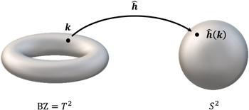
Figure 1. Topological map from the base manifold (k-space, Brillouin zone) to the group space, $\hat{{\boldsymbol{h}}}:{T}^{2}\to {S}^{2}$. |
| • | hx = hy = hz = 0, yielding $\begin{eqnarray}\begin{array}{l}E=\parallel {\boldsymbol{h}}\parallel =0\qquad \mathrm{and}\\ \parallel {\boldsymbol{h}}\parallel \mp {h}_{z}=0,\end{array}\end{eqnarray}$ corresponding to the center O of the sphere S2 in the group space, as shown in figure 2. In the forthcoming sections it will be pointed out that equation ( |
| • | hx = hy = 0 and hz ≠ 0, yielding $\parallel {\boldsymbol{h}}\parallel \ne 0$ and $\begin{eqnarray}\begin{array}{l}\mathrm{when}\ E=+\parallel {\boldsymbol{h}}\parallel :\parallel {\boldsymbol{h}}\parallel -{h}_{z}=0,\\ {\rm{i}}.{\rm{e}}.\quad {\hat{h}}_{z}=+1;\end{array}\end{eqnarray}$ $\begin{eqnarray}\begin{array}{l}\mathrm{when}\ E=-\parallel {\boldsymbol{h}}\parallel :\parallel {\boldsymbol{h}}\parallel +{h}_{z}=0,\\ {\rm{i}}.{\rm{e}}.\quad {\hat{h}}_{z}=-1,\end{array}\end{eqnarray}$ where an ${\hat{h}}_{z}$ is introduced for convenience, ${\hat{h}}_{z}=\tfrac{{h}_{z}}{\parallel {\boldsymbol{h}}\parallel }$. Equations ( |

Figure 2. Sphere S2 in the group space formed by the three-dimensional unit vector $\hat{{\boldsymbol{h}}}$. $\left\{{\hat{{\boldsymbol{e}}}}_{1},{\hat{{\boldsymbol{e}}}}_{2},{\hat{{\boldsymbol{e}}}}_{3}\right\}$ is an orthonormal frame. The center is O, where monopole defects take place. The north-pole is N, where $E={h}_{z}=\parallel {\boldsymbol{h}}\parallel \ne 0;$ the south-pole is S, where $E={h}_{z}=-\parallel {\boldsymbol{h}}\parallel \ne 0$. At N and S there is hx = hy = 0, hence meron defects take place, with the topological charges given by the winding numbers of the vector fields in the local Euclidean charts. See section |
3. Gauge theory
4. Monopoles and merons: with typical example
4.1. Monopoles and merons
| • | In the group space, the double integral on the closed surface S2, ${\int }_{{S}^{2}}K$, could be turned into a triple integral over a body B3 via the Stokes theorem: $\begin{eqnarray}\begin{array}{l}\displaystyle \frac{1}{4\pi }{\displaystyle \int }_{{S}^{2}}K=\displaystyle \frac{1}{4\pi }{\displaystyle \int }_{{S}^{2}}\hat{{\boldsymbol{h}}}\cdot \left({\rm{d}}\hat{{\boldsymbol{h}}}\times {\rm{d}}\hat{{\boldsymbol{h}}}\right)\\ =\displaystyle \frac{1}{4\pi }{\displaystyle \int }_{{B}^{3}}{\rm{d}}\hat{{\boldsymbol{h}}}\cdot \left({\rm{d}}\hat{{\boldsymbol{h}}}\times {\rm{d}}\hat{{\boldsymbol{h}}}\right)\\ =\displaystyle \frac{1}{4\pi }{\displaystyle \int }_{{B}^{3}}\left(-\displaystyle \frac{2}{{\parallel {\boldsymbol{h}}\parallel }^{3}}\right){\rm{d}}{\boldsymbol{h}}\cdot \left({\rm{d}}{\boldsymbol{h}}\times {\rm{d}}{\boldsymbol{h}}\right)\\ =\displaystyle \frac{1}{4\pi }{\displaystyle \int }_{{B}^{3}}{{\rm{\nabla }}}^{2}\displaystyle \frac{1}{\parallel {\boldsymbol{h}}\parallel }{\rm{d}}V,\end{array}\end{eqnarray}$ where B3 is the unit ball in three dimensions, with boundary ∂B3 = S2. The volume element reads ${\rm{d}}V={\rm{d}}{\boldsymbol{h}}\cdot \left({\rm{d}}{\boldsymbol{h}}\times {\rm{d}}{\boldsymbol{h}}\right)=\tfrac{1}{3!}{\epsilon }_{{abc}}{\rm{d}}{h}_{a}\wedge {\rm{d}}{h}_{b}\wedge {\rm{d}}{h}_{c}$. The integrand ${{\rm{\nabla }}}^{2}\tfrac{1}{\parallel {\boldsymbol{h}}\parallel }$ is the Laplacian of a point-source potential, ${{\rm{\nabla }}}^{2}\tfrac{1}{\parallel {\boldsymbol{h}}\parallel }=4\pi {\delta }^{3}\left({\boldsymbol{h}}\right)$. Thus, $\begin{eqnarray}\displaystyle \frac{1}{4\pi }{\int }_{{S}^{2}}K={\int }_{{B}^{3}}{\delta }^{3}\left({\boldsymbol{h}}\right){\rm{d}}V=1.\end{eqnarray}$ In equation ( |
| • | However, from the angle of view of the base manifold T2, the 3-form ${\rm{d}}\hat{{\boldsymbol{h}}}\cdot \left({\rm{d}}\hat{{\boldsymbol{h}}}\times {\rm{d}}\hat{{\boldsymbol{h}}}\right)$ cannot be pulled back to a triple integral, because T2 lacks the third coordinate beyond kx and ky. This corresponds to an indeterminate evaluation for the Chern number C. That is, when the monopole excitations occur at h = 0, the insulator experiences a topological transition with the Chern number C taking an indeterminate value. |

Figure 3. Orthonormal frame $\left\{\hat{{\boldsymbol{h}}},\hat{{\boldsymbol{e}}},\hat{{\boldsymbol{f}}}\right\}$: the unit vector $\hat{{\boldsymbol{h}}}$ forms a 2-sphere S2 in the ${SU}\left(2\right)$ group space, while $\hat{{\boldsymbol{e}}}$ and $\hat{{\boldsymbol{f}}}$ are two perpendicular unit vectors on the S2. The base manifold chosen to perform this technique of Wu–Yang potential is a hemisphere, identical to a local Euclidean chart. |
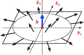
Figure 4. Neighborhood of the pole N, where the vector h is parallel to the ${\hat{{\boldsymbol{e}}}}_{3}$-axis, with hx = hy = 0. The winding number of the vector $\left({h}_{x},{h}_{y}\right)$ in the two-dimensional vicinity of N gives the topological charge of the meron. |
4.2. Typical example
| i | (i)Monopoles: They occur at the Dirac points with $E=\parallel {\boldsymbol{h}}\parallel =0$. The solutions of the zero point equations $\begin{eqnarray}{h}_{x}={h}_{y}={h}_{z}=0\end{eqnarray}$ give the locations of the monopole defects: $\left({k}_{x},{k}_{y}\right)=\left(0,0\right)$, with m = −2, due to equation ( $\left({k}_{x},{k}_{y}\right)=\left(0,\pi \right)$ and $\left(\pi ,0\right)$, with m = 0; $\left({k}_{x},{k}_{y}\right)=\left(\pi ,\pi \right)$, with m = 2. |
| ii | (ii)Merons: They occur at the two-dimensional singular points where $\begin{eqnarray}{h}_{x}={h}_{y}=0,\qquad E={h}_{z}=\pm \parallel {\boldsymbol{h}}\parallel \ne 0.\end{eqnarray}$ |
Table 1. Locations of the meron defects of the ∣C∣ = 1 model, and the corresponding m values, where hx = hy = 0 and $E={h}_{z}=\pm \sqrt{\parallel {\boldsymbol{h}}\parallel }\ne 0$. |
| Moment kx | Moment ky | On-site energy m | hz i.e. E |
|---|---|---|---|
| 0 | 0 | m ≠ −2 | m + 2 |
| 0 | π | m ≠ 0 | m |
| π | 0 | m ≠ 0 | m |
| π | π | m ≠ 2 | m − 2 |
| • | Near kx = 0: ${h}_{x}=\sin {k}_{x}\approx {\rm{\Delta }}{k}_{x}$, where Δkx = kx − 0. Similarly, near ky = 0: hy ≈ Δky, where Δky = ky − 0. |
| • | Near kx = π: ${h}_{x}=\sin {k}_{x}\approx \pi -{\rm{\Delta }}{k}_{x}$, where Δkx = kx − π. Similarly, near ky = π: hy ≈ π − Δky, where Δky = ky − π. |
| • | Near $\left({k}_{x},{k}_{y}\right)=(0,0)$, the asymptotic behavior of $\left({h}_{x},{h}_{y}\right)$ is $\left({\rm{\Delta }}{k}_{x},{\rm{\Delta }}{k}_{y}\right)$. Such a vector field distribution represents a source-point, so the winding number is +1. |
| • | Near $\left({k}_{x},{k}_{y}\right)=(0,\pi )$, that of $\left({h}_{x},{h}_{y}\right)$ is $\left({\rm{\Delta }}{k}_{x},-{\rm{\Delta }}{k}_{y}\right)$. This is a saddle-point, with winding number −1. |
| • | Near $\left({k}_{x},{k}_{y}\right)=(\pi ,0)$, that of $\left({h}_{x},{h}_{y}\right)$ is $\left(-{\rm{\Delta }}{k}_{x},{\rm{\Delta }}{k}_{y}\right)$. This is a saddle-point, with winding number −1. |
| • | Near $\left({k}_{x},{k}_{y}\right)=(\pi ,\pi )$, that of $\left({h}_{x},{h}_{y}\right)$ is $\left(-{\rm{\Delta }}{k}_{x},-{\rm{\Delta }}{k}_{y}\right)$. This is a congruence-point, with winding number +1. |
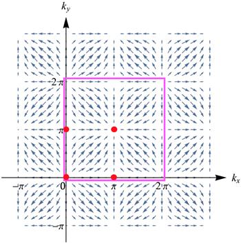
Figure 5. Merons, i.e. two dimensional point defects, of the ∣C∣ = 1 model, marked as red spots: (0, 0) and (π, π) are source/congruence points, so they have a winding number +1; (0, π) and (π, 0) are saddle points, so they have a winding number −1. The pink-boxed region indicates the first Brillouin zone. |
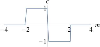
Figure 6. The different evaluations of the Chern number C of the ∣C∣ = 1 model due to varying on-site energy m, as described by [9]. This figure is produced by directly substituting equation ( |
Table 2. Winding numbers at the meron defects of the ∣C∣ = 1 model, and their total contribution to the north pole N (${\hat{h}}_{z}$ = +1). |
| On-site energy m | $\left(0,0\right)$ | $\left(0,\pi \right)$ | $\left(\pi ,0\right)$ | $\left(\pi ,\pi \right)$ | Total contribution to N, i.e. CN |
|---|---|---|---|---|---|
| m > 2 | +1 | −1 | −1 | +1 | 0 |
| 0 < m < 2 | +1 | −1 | −1 | / | −1 |
| −2 < m < 0 | +1 | / | / | / | +1 |
| m < −2 | / | / | / | / | 0 |
Table 3. Winding numbers at the meron defects of the ∣C∣ = 1 model, and their total contribution to the south pole S (${\hat{h}}_{z}$ = −1). |
| On-site energy m | $\left(0,0\right)$ | $\left(0,\pi \right)$ | $\left(\pi ,0\right)$ | $\left(\pi ,\pi \right)$ | Total contribution to S, i.e. CS |
|---|---|---|---|---|---|
| m > 2 | / | / | / | / | 0 |
| 0 < m < 2 | / | / | / | +1 | +1 |
| −2 < m < 0 | / | −1 | −1 | +1 | −1 |
| m < −2 | +1 | −1 | −1 | +1 | 0 |
| • | When m > 2: |
| 1. At (kx, ky) = (0, 0): according to equation ( | |
| 2. At (kx, ky) = (0, π) and (π, 0): according to equation ( | |
| 3. At (kx, ky) = (π, π): hz = m − 2 > 0, hence hz = +∥h∥ and ${\hat{h}}_{z}=\tfrac{{h}_{z}}{\parallel {\boldsymbol{h}}\parallel }$ = +1, the north-pole. This means the topological charge +1 of (kx, ky) = (π, π) has contribution to N. |
| • | When 0 < m < 2: |
| 1. At (kx, ky) = (0, 0): hz = m + 2 > 0, hence ${\hat{h}}_{z}$ = +1, the north-pole. This means the topological charge +1 of (kx, ky) = (0, 0) has contribution to N. | |
| 2. At (kx, ky) = (0, π) and (π, 0): hz = m > 0, hence ${\hat{h}}_{z}$ = +1, the north-pole. This means both the topological charges of (0, π) and (π, 0), −1 − 1 = −2, have contributions to N. | |
| 3. At (kx, ky) = (π, π): hz = m − 2 < 0, hence hz = − ∥h∥ and ${\hat{h}}_{z}=\tfrac{{h}_{z}}{\parallel {\boldsymbol{h}}\parallel }$ = −1, the south-pole. This means the topological charge +1 of (kx, ky) = (π, π) has contribution to the south-pole S. |
| • | When −2 < m < 0: |
| 1. At (kx, ky) = (0, 0): hz = m + 2 > 0, hence ${\hat{h}}_{z}$ = +1, the north-pole. This means the topological +1 charge of (kx, ky) = (0, 0) has contribution to N. | |
| 2. At (kx, ky) = (0, π) and (π, 0): hz = m < 0, hence ${\hat{h}}_{z}$ = −1, the south-pole. This means both the topological charges of (0, π) and (π, 0), −1 − 1 = −2, have contributions to S. | |
| 3. At (kx, ky) = (π, π): hz = m − 2 < 0, hence ${\hat{h}}_{z}$ = −1, the south-pole. This means the topological charge +1 of (kx, ky) = (π, π) has contribution to S. |
| • | When m < −2: |
| 1. At (kx, ky) = (0, 0): hz = m + 2 < 0, hence ${\hat{h}}_{z}$ = −1, the south-pole. This means the topological charge +1 of (kx, ky) = (0, 0) has contribution to S. | |
| 2. At (kx, ky) = (0, π) and (π, 0): hz = m < 0, hence ${\hat{h}}_{z}$ = −1, the south-pole. This means both the topological charges of (0, π) and (π, 0), −1 − 1 = −2, have contributions to S. | |
| 3. At (kx, ky) = (π, π): hz = m − 2 < 0, hence ${\hat{h}}_{z}$ = −1, the south-pole. This means the topological charge +1 of (kx, ky) = (π, π) has contribution to S. |
5. Berry connection and Chern number of merons: with example
6. Higher Chern number insulator and corresponding topological defects
| i | (i)Monopoles: Monopole defects occur at the Dirac points with E = ∥h∥ = 0. The solutions of the zero point equations $\begin{eqnarray}{h}_{x}={h}_{y}={h}_{z}=0\end{eqnarray}$ |
Table 4. Locations of the monopole defects of the high-C model, and the corresponding m values, where hx = hy = hz = 0. |
 |
| i | (ii)Merons: Meron defects occur at the two-dimensional singular points where $\begin{eqnarray}{h}_{x}={h}_{y}=0,\qquad E={h}_{z}=\pm \parallel {\boldsymbol{h}}\parallel \ne 0.\end{eqnarray}$ |
Table 5. Locations of the meron defects of the high-C model, and the corresponding m values, where hx = hy = 0 and $E={h}_{z}=\pm \sqrt{\parallel {\boldsymbol{h}}\parallel }\ne 0$. |
 |
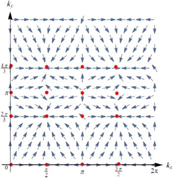
Figure 7. Merons in the high-C model, marked as red spots: (0, 0), (0, π), (π, 0) and (π, π) are the source points, each having a winding number +1; (π/2, 2π/3), (π/2, 4π/3), (3π/2, 2π/3) and (3π/2, 4π/3) are the congruence points, each having a winding number +1; (0, 2π/3), (0, 4π/3), (π/2, 0), (π/2, π), (π, 2π/3), (π, 4π/3), (3π/2, 0) and (3π/2, π) are the saddle points, each having a winding number −1. |
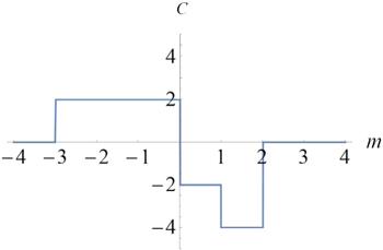
Figure 8. The different evaluations of the Chern number C of the high-C model due to varying on-site energy m. This figure is produced by directly substituting equation ( |
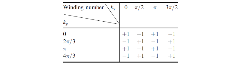
Table 6. The winding numbers at the meron defects in the high-C model. |
 |
| • | When m > 2: all topological charges have contributions to the north-pole N, but no contributions to the south-pole S. Thus, CN = CS = 0. |
| • | When 1 < m < 2: the topological charges of (0, 0), (0, 2π/3), (0, π), (0, 4π/3), (π/2, 0), (π/2, π), (π, 0), (π, 2π/3), (π, π), (π, 4π/3), (3π/2, 0), (3π/2, π) have contributions to the north-pole N, while the others have contributions to the south-pole S. Thus, CN = −4, CS = +4. |
| • | When 0 < m < 1: the topological charges of (0, 0), (0, 2π/3), (0, π), (0, 4π/3), (π/2, 0), (π, 0), (π, 2π/3), (π, π), (π, 4π/3), (3π/2, 0) have contribution to the north-pole N, while the others have contribution to the south-pole S. Thus, CN = −2, CS = + 2. |
| • | When −1 < m < 0: the topological charges of (0, 0), (0, π), (π/2, 0), (π, 0), (π, π), (3π/2, 0) have contributions to the north-pole N, while the others have contributions to the south-pole S. Thus, CN = +2, CS = −2. |
| • | When −3 < m < −1: the topological charges of (0, 0), (π, 0) have contributions to the north-pole N, while the others have contributions to the south-pole S. Thus, CN = +2, CS = −2. |
| • | When m < −3: all the topological charges have contributions to the south-pole S, but no contributions to the north-pole N. Thus CN = CS = 0. |