Welcome to visit Communications in Theoretical Physics,
Mathematical Physics

The Sharma-Tasso-Olver-Burgers equation: its conservation laws and kink solitons

  • K Hosseini , 1 ,
  • A Akbulut 2 ,
  • D Baleanu 3, 4 ,
  • S Salahshour 5
Expand
  • 1Department of Mathematics, Near East University TRNC, Mersin 10, Turkey
  • 2Department of Mathematics-Computer, Art-Science Faculty, Eskisehir Osmangazi University, Eskisehir, Turkey
  • 3Department of Mathematics, Faculty of Arts and Sciences, Cankaya University, Ankara 06530, Turkey
  • 4Institute of Space Sciences, Magurele-Bucharest, Romania
  • 5Faculty of Engineering and Natural Sciences, Bahcesehir University, Istanbul, Turkey

Received date: 2021-09-17

  Revised date: 2021-12-16

  Accepted date: 2021-12-17

  Online published: 2022-03-10

Copyright

© 2022 Institute of Theoretical Physics CAS, Chinese Physical Society and IOP Publishing

Abstract

The present paper deals with the Sharma–Tasso–Olver–Burgers equation (STOBE) and its conservation laws and kink solitons. More precisely, the formal Lagrangian, Lie symmetries, and adjoint equations of the STOBE are firstly constructed to retrieve its conservation laws. Kink solitons of the STOBE are then extracted through adopting a series of newly well-designed approaches such as Kudryashov and exponential methods. Diverse graphs in 2 and 3D postures are formally portrayed to reveal the dynamical features of kink solitons. According to the authors’ knowledge, the outcomes of the current investigation are new and have been listed for the first time.

Cite this article

K Hosseini , A Akbulut , D Baleanu , S Salahshour . The Sharma-Tasso-Olver-Burgers equation: its conservation laws and kink solitons[J]. Communications in Theoretical Physics, 2022 , 74(2) : 025001 . DOI: 10.1088/1572-9494/ac4411

1. Introduction

Partial differential equations (PDEs) particularly their nonlinear regimes are applied to model a wide variety of phenomena in the extensive areas of science and engineering. As useful tools for simulating many nonlinear phenomena, such models play a pivotal role in progressing the real world. During the past few decades, one of the major goals has been the construction of novel approaches to extract solitons for PDEs. In the last years, several well-organized methods have been proposed to derive solitons of PDEs, the hyperbolic function method [14], the modified Jacobi methods [58], the Kudryashov method [914], and the exponential method [1520], are samples to point out.
It is noteworthy that all conservation laws of PDEs do not include physical meanings, however, such laws are essential to explore the integrability and reduction of PDEs [21, 22]. Conservation laws of PDEs can be found by using a wide range of methods such as the multiplier approach, the Noether approach, the new conservation theorem, and so on. Of these, the new conservation theorem was first established by Ibragimov and is associated with the formal Lagrangian, Lie symmetries, and adjoint equations of PDEs. Conservation laws can be derived for every symmetry of PDEs and the obtained conservation laws are referred to as trivial or non-trivial [2329].
In the present study, the authors deal with the following Sharma–Tasso–Olver–Burgers equation [30]
$\begin{eqnarray}\begin{array}{l}{u}_{t}+{c}_{1}\left(3{u}_{x}^{2}+3{u}^{2}{u}_{x}+3u{u}_{xx}+{u}_{xxx}\right)+{c}_{2}\left(2u{u}_{x}+{u}_{xx}\right)\,=\,0,\end{array}\end{eqnarray}$
and derive its conservation laws and kink solitons. As is clear from the name of equation (1), such a model consists of the Sharma–Tasso–Olver and Burgers equations. These equations have been the main concern of a lot of research works. Or-Roshid and Rashidi [31] employed an exponential method to derive the solitons of these equations. In another investigation, multiple solitons of these equations were obtained by Wazwaz in [32] through the simplified Hirota’s method. Very recently, Hu et al [33] constructed soliton, lump, and interaction solutions of a 2D-STOBE using a series of systematic ansatzes.
Kudryashov and exponential methods, as privileged approaches, have been applied by many scholars to retrieve solitons of PDEs. Particularly, the effectiveness of these methods has been demonstrated by Hosseini et al in several papers. Hosseini et al [34] derived solitons of the cubic-quartic nonlinear Schrödinger equation using the Kudryashov method. The exponential method was utilized in [35] by Hosseini et al to acquire solitons of the unstable nonlinear Schrödinger equation.
The rest of the current study is as follows: In section 2, the conservation theorem and the foundation of Kudryashov and exponential methods are given. In section 3, the formal Lagrangian, Lie symmetries, and adjoint equations of the STOBE are established to derive its conservation laws. In section 4, Kudryashov and exponential methods are adopted to seek solitons of the STOBE. Section 4 further gives diverse graphs in 2 and 3D postures to demonstrate the dynamical features of kink solitons. The achievements of the present paper are provided in section 5.

2. The conservation theorem and methods

In the current section, the conservation theorem and the foundation of Kudryashov and exponential methods are formally given.

2.1. The conservation theorem

To start, suppose that a PDE can be expressed as
$\begin{eqnarray}P(u,{u}_{x},{u}_{t},\mathrm{...})=0,\end{eqnarray}$
where $P$ is a polynomial. The Lie point symmetry generator of equation (2) is given by
$\begin{eqnarray}\begin{array}{l}X={\xi }^{x}\left(x,t,u\right)\displaystyle \frac{\partial }{\partial x}+{\xi }^{t}\left(x,t,u\right)\displaystyle \frac{\partial }{\partial t}\\ \,\,+\,\eta \left(x,t,u\right)\displaystyle \frac{\partial }{\partial u},\end{array}\end{eqnarray}$
where ${\xi }^{x}\left(x,t,u\right),$ ${\xi }^{t}\left(x,t,u\right),$ and $\eta \left(x,t,u\right)$ are known as the infinitesimals. The kth prolongation of equation (3) is retrieved by
$\begin{eqnarray*}{X}^{\left(k\right)}=X+{\eta }_{i}^{\left(1\right)}\displaystyle \frac{\partial }{\partial {u}_{i}^{\alpha }}+\mathrm{...}+{\eta }_{{i}_{1}{i}_{2}\mathrm{...}{i}_{k}}^{\left(k\right)}\displaystyle \frac{\partial }{\partial {u}_{{i}_{1}{i}_{2}\mathrm{...}{i}_{k}}},k\geqslant 1,\end{eqnarray*}$
where
$\begin{eqnarray*}{\eta }_{i}^{\left(1\right)}={D}_{i}\eta -\left({D}_{i}{\xi }^{j}\right){u}_{j},\end{eqnarray*}$
$\begin{eqnarray*}{\eta }_{{i}_{1}{i}_{2}\mathrm{...}{i}_{k}}^{\left(k\right)}={D}_{{i}_{k}}{\eta }_{{i}_{1}{i}_{2}\mathrm{...}{i}_{k-1}}^{\left(k-1\right)}-\left({D}_{{i}_{k}}{\xi }^{j}\right){u}_{{i}_{1}{i}_{2}\mathrm{...}{i}_{k-1}j}.\end{eqnarray*}$
Above $i,j=1,2$ and ${i}_{l}=1$ for $l=1,2,\mathrm{...},k.$ The total derivative operator is indicated by ${D}_{i}.$
The formal Lagrangian is given by multiplying equation (2) by $w$ as follows
$\begin{eqnarray*}L=wP,\end{eqnarray*}$
where $w$ is the adjoint variable. It is noteworthy that the adjoint equation is retrieved by
$\begin{eqnarray}P* \,=\,\displaystyle \frac{\delta L}{\delta u},\end{eqnarray}$
where $\tfrac{\delta }{\delta u}$ is the variational derivative.
If the solution of equation (4) is found, then, a finite number of conservation laws for equation (2) are derived.

Every Lie point, Lie-Bäcklund, and nonlocal symmetry of equation (2) results in a conservation law. The components of the conserved vector are given by [29]

$\begin{eqnarray}{T}^{i}={\xi }^{i}L+W\,\frac{\delta L}{\delta {u}_{i}}+\displaystyle \sum _{s\geqslant 1}{D}_{{i}_{1}}\ldots {D}_{{i}_{s}}(W)\frac{\delta L}{\delta {u}_{i{i}_{1}{i}_{2}\mathrm{...}{i}_{s}}},\end{eqnarray}$
where $W=\eta -{\xi }^{j}{u}_{j},$ and ${\xi }^{i}\,$ and $\eta $ are the infinitesimal functions. The conserved vectors generated by equation (5) consist of the arbitrary solutions of the adjoint equation. Consequently, one derives a finite number of conservation laws for equation (2) by $w$ [36].

Derived conserved vectors using (5) are conservation laws of equation (2) if

$\begin{eqnarray*}{D}_{i}\left({T}^{i}\right)=0.\end{eqnarray*}$
Here, ${D}_{i}$ is referred to as the total derivative [37].

2.2. Foundation of methods

The Kudryashov method applies the following series [9, 10]
$\begin{eqnarray}\begin{array}{l}U\left({\epsilon }\right)={a}_{0}+{a}_{1}K\left({\epsilon }\right)+{a}_{2}{K}^{2}\left({\epsilon }\right)+\ldots \\ \,\,\,+\,{a}_{N}{K}^{N}\left({\epsilon }\right),\,{a}_{N}\ne 0,\end{array}\end{eqnarray}$
as the nontrivial solution of
$\begin{eqnarray}O\left(U\left({\epsilon }\right),U^{\prime} \left({\epsilon }\right),U^{\prime\prime} \left({\epsilon }\right),\ldots \right)=0.\end{eqnarray}$
Above, ${a}_{i},i=0,1,\mathrm{...},N$ are unknowns, $N$ is retrieved by the balance approach, and
$\begin{eqnarray*}K\left({\epsilon }\right)=\displaystyle \frac{1}{1+d{a}^{{\epsilon }}}\end{eqnarray*}$
is the solution of
$\begin{eqnarray*}K^{\prime} \left({\epsilon }\right)=K\left({\epsilon }\right)\left(K\left({\epsilon }\right)-1\right)\mathrm{ln}\left(a\right).\end{eqnarray*}$
Equations (6) and (7) together result in a nonlinear system which by solving it, solitons of equation (7) are derived.
The exponential method investigates a solution for equation (7) as [15, 16]
$\begin{eqnarray}\begin{array}{l}U\left({\epsilon }\right)=\displaystyle \frac{{a}_{0}+{a}_{1}{a}^{{\epsilon }}+{a}_{2}{a}^{2{\epsilon }}+\ldots +{a}_{N}{a}^{N{\epsilon }}}{{b}_{0}+{b}_{1}{a}^{{\epsilon }}+{b}_{2}{a}^{2{\epsilon }}+\ldots +{b}_{N}{a}^{N{\epsilon }}},\\ {a}_{N}\ne 0,\,{b}_{N}\ne 0,\end{array}\end{eqnarray}$
where the unknowns are acquired later and $N\in {{\mathbb{Z}}}^{+}.$
Again, equations (7) and (8) together yield a nonlinear system which by solving it, solitons of equation (7) are obtained.

3. The STOBE and its conservation laws

In the present section, the conservation theorem is applied to the STOBE to derive its conservation laws. First, the formal Lagrangian is derived in the following form
$\begin{eqnarray}\begin{array}{l}L=w\left({u}_{t}+{c}_{1}\left(3{u}_{x}^{2}+3{u}^{2}{u}_{x}+3u{u}_{xx}+{u}_{xxx}\right)\right.\\ \,\,+\,\left.{c}_{2}\left(2u{u}_{x}+{u}_{xx}\right)\right),\end{array}\end{eqnarray}$
where $w$ is the adjoint variable.
The adjoint equation is acquired with the aid of the variational derivative as
$\begin{eqnarray}\begin{array}{l}F* \,=\,-{w}_{t}+{c}_{1}\left(-3{u}^{2}{w}_{x}+3u{w}_{xx}-{w}_{xxx}\right)\\ \,\,+\,{c}_{2}\left({w}_{xx}-2u{w}_{x}\right).\end{array}\end{eqnarray}$
If $u$ is replaced by $w$ in equation (10), then, equation (1) is not obtained. Thus, equation (1) is not self-adjoint. In such a case, one can say that $w=1$ is a solution of equation (10).
A one-parameter Lie group for equation (1) is given by
$\begin{eqnarray*}x\to x+\varepsilon {\xi }^{x}\left(x,t,u\right),\end{eqnarray*}$
$\begin{eqnarray*}t\to t+\varepsilon {\xi }^{t}\left(x,t,u\right),\end{eqnarray*}$
$\begin{eqnarray*}u\to u+\varepsilon \eta \left(x,t,u\right),\end{eqnarray*}$
where $\varepsilon $ is the group parameter, and consequently equation (1) admits following Lie point symmetry generator
$\begin{eqnarray*}X={\xi }^{x}\displaystyle \frac{\partial }{\partial x}+{\xi }^{t}\displaystyle \frac{\partial }{\partial t}+\eta \displaystyle \frac{\partial }{\partial u}.\end{eqnarray*}$
Obviously, $X$ must be satisfied the Lie symmetry condition as follow
$\begin{eqnarray*}\begin{array}{l}{X}^{\left(3\right)}\left({u}_{t}+{c}_{1}\left(3{u}_{x}^{2}+3{u}^{2}{u}_{x}+3u{u}_{xx}+{u}_{xxx}\right)\right.\\ \,+\left.{c}_{2}\left(2u{u}_{x}+{u}_{xx}\right)\right)=0.\end{array}\end{eqnarray*}$
The third prolongation of the Lie point symmetry generator is given by
$\begin{eqnarray*}\begin{array}{l}{X}^{\left(3\right)}={\xi }^{x}\displaystyle \frac{\partial }{\partial x}+{\xi }^{t}\displaystyle \frac{\partial }{\partial t}+\eta \displaystyle \frac{\partial }{\partial u}+{\eta }^{x}\displaystyle \frac{\partial }{\partial {u}_{x}}\\ \,\,+\,{\eta }^{t}\displaystyle \frac{\partial }{\partial {u}_{t}}+{\eta }^{xx}\displaystyle \frac{\partial }{\partial {u}_{xx}}+{\eta }^{xxx}\displaystyle \frac{\partial }{\partial {u}_{xxx}},\end{array}\end{eqnarray*}$
where
$\begin{eqnarray*}{\eta }^{x}={D}_{x}\left(\eta \right)-{u}_{x}{D}_{x}\left({\xi }^{x}\right)-{u}_{t}{D}_{x}\left({\xi }^{t}\right),\end{eqnarray*}$
$\begin{eqnarray*}{\eta }^{t}={D}_{t}\left(\eta \right)-{u}_{x}{D}_{t}\left({\xi }^{x}\right)-{u}_{t}{D}_{t}\left({\xi }^{t}\right),\end{eqnarray*}$
$\begin{eqnarray*}{\eta }^{xx}={D}_{x}\left({\eta }^{x}\right)-{u}_{xx}{D}_{x}\left({\xi }^{x}\right)-{u}_{xt}{D}_{x}\left({\xi }^{t}\right),\end{eqnarray*}$
$\begin{eqnarray*}{\eta }^{xxx}={D}_{x}\left({\eta }^{xx}\right)-{u}_{xxx}{D}_{x}\left({\xi }^{x}\right)-{u}_{xxt}{D}_{x}\left({\xi }^{t}\right).\end{eqnarray*}$
If we apply ${X}^{\left(3\right)}$ to equation (1), an equivalent condition is obtained as
$\begin{eqnarray*}\begin{array}{l}{\eta }^{t}+{c}_{1}\left(6{u}_{x}{\eta }^{x}+6u\eta {u}_{x}+3{u}^{2}{\eta }^{x}+3\eta {u}_{xx}+3u{\eta }^{xx}+{\eta }^{xxx}\right)\\ \,+{c}_{2}\left(2\eta {u}_{x}+2u{\eta }^{x}+{\eta }^{xx}\right)=0.\end{array}\end{eqnarray*}$
Now, after some operations, we find the infinitesimal functions as follows
$\begin{eqnarray*}\begin{array}{l}{\xi }^{t}={k}_{1}+{k}_{3}t,\,{\xi }^{x}={k}_{2}+{k}_{3}\left(\displaystyle \frac{3{c}_{1}x-2{c}_{2}^{2}t}{9{c}_{1}}\right),\\ \eta ={k}_{3}\left(\displaystyle \frac{-3{c}_{1}u-{c}_{2}}{9{c}_{1}}\right),\end{array}\end{eqnarray*}$
where ${k}_{1},$ ${k}_{2},$ and ${k}_{3}$ are arbitrary constants. Finally, the Lie point symmetry generators of equation (1) are given by
$\begin{eqnarray}\begin{array}{l}{X}_{1}=\displaystyle \frac{\partial }{\partial t},\,{X}_{2}=\displaystyle \frac{\partial }{\partial x},\,{X}_{3}=\left(\displaystyle \frac{3{c}_{1}x-2{c}_{2}^{2}t}{9{c}_{1}}\right)\displaystyle \frac{\partial }{\partial x}\\ \,\,+\,t\displaystyle \frac{\partial }{\partial t}+\left(\displaystyle \frac{-3{c}_{1}u-{c}_{2}}{9{c}_{1}}\right)\displaystyle \frac{\partial }{\partial u}.\end{array}\end{eqnarray}$
The commutator table for the above symmetries (see equation (11)) has been given in table 1.
Table 1. The commutator table for the above symmetries.
$[{X}_{i},{X}_{j}]$ ${X}_{1}$ ${X}_{2}$ ${X}_{3}$
${X}_{1}$ $0$ $0$ ${X}_{1}-\tfrac{2{c}_{2}^{2}}{9{c}_{1}}{X}_{2}$
${X}_{2}$ $0$ $0$ $\tfrac{{X}_{2}}{3}$
${X}_{3}$ $-{X}_{1}+\tfrac{2{c}_{2}^{2}}{9{c}_{1}}{X}_{2}$ $-\tfrac{{X}_{2}}{3}$ $0$
Now, conservation laws of the STOBE for all founded Lie point symmetry generators are derived. Conservation laws formulae for equation (1) are as follows
$\begin{eqnarray}\begin{array}{l}{T}^{x}={\xi }^{x}L+W\left[\displaystyle \frac{\partial L}{\partial {u}_{x}}-{D}_{x}\left(\displaystyle \frac{\partial L}{\partial {u}_{xx}}\right)+{D}_{x}^{2}\left(\displaystyle \frac{\partial L}{\partial {u}_{xxx}}\right)\right]\\ \,+{D}_{x}\left(W\right)\left[\displaystyle \frac{\partial L}{\partial {u}_{xx}}-{D}_{x}\left(\displaystyle \frac{\partial L}{\partial {u}_{xxx}}\right)\right]+{D}_{x}^{2}\left(W\right)\left[\displaystyle \frac{\partial L}{\partial {u}_{xxx}}\right],\end{array}\end{eqnarray}$
$\begin{eqnarray}{T}^{t}={\xi }^{t}L+W\left(\displaystyle \frac{\partial L}{\partial {u}_{t}}\right).\end{eqnarray}$

If we employ (12) and (13) to equation (9) with the use of ${X}_{1},$ we acquire the following conservation laws

$\begin{eqnarray*}\begin{array}{l}{T}_{1}^{x}=-3{c}_{1}\left({u}_{t}w{u}_{x}+{u}_{t}w{u}^{2}+{u}_{xt}uw\right)-2{c}_{2}{u}_{t}wu\\ \,-{c}_{2}{u}_{xt}w+{c}_{1}\left(3{u}_{t}u{w}_{x}-{u}_{t}{w}_{xx}+{u}_{xt}{w}_{x}-{u}_{xxt}w\right)\\ \,+{c}_{2}{u}_{t}{w}_{x},\\ {T}_{1}^{t}=3{c}_{1}\left({u}^{2}{u}_{x}w+wu{u}_{xx}+w{u}_{x}^{2}\right)+{c}_{2}w\left(2u{u}_{x}+{u}_{xx}\right)\\ \,\,+\,{c}_{1}w{u}_{xxx}.\end{array}\end{eqnarray*}$
Due to the satisfaction of the divergence condition, these conservation laws are called local conservation laws. Such conservation laws are infinite trivial conservation laws. In this case, we have
$\begin{eqnarray*}{D}_{x}\left({T}_{1}^{x}\right)+{D}_{t}\left({T}_{1}^{t}\right)={u}_{t}{w}_{t}-{u}_{t}{w}_{t}=0.\end{eqnarray*}$
It is noted that for $w=1,$ from ${T}_{1}^{x}$ and ${T}_{1}^{t},$ one can find
$\begin{eqnarray}\begin{array}{l}\tilde{{T}_{1}^{x}}=-3{c}_{1}{u}^{2}{u}_{t}-3{c}_{1}u{u}_{xt}-3{c}_{1}{u}_{x}{u}_{t}-2{c}_{2}u{u}_{t}\\ \,\,-\,{c}_{2}{u}_{xt}-{c}_{1}{u}_{xxt},\end{array}\end{eqnarray}$
$\begin{eqnarray}\begin{array}{l}\tilde{{T}_{1}^{t}}=3{c}_{1}{u}^{2}{u}_{x}+3{c}_{1}u{u}_{xx}+3{c}_{1}{u}_{x}^{2}+2{c}_{2}u{u}_{x}+{c}_{2}{u}_{xx}\\ \,\,+\,{c}_{1}{u}_{xxx}.\end{array}\end{eqnarray}$
Finite conserved vectors (14) and (15) satisfy the divergence condition, so they are trivial conservation laws.

If we apply (12) and (13) to equation (9) with the aid of ${X}_{2},$ we find the following local conservation laws

$\begin{eqnarray*}\begin{array}{l}{T}_{2}^{x}={c}_{1}{u}_{xx}{w}_{x}-{c}_{1}{u}_{x}{w}_{xx}+{u}_{x}{w}_{x}\left(3{c}_{1}u+{c}_{2}\right)\,+\,w{u}_{t},\\ {T}_{2}^{t}=-w{u}_{x}.\end{array}\end{eqnarray*}$
Owing to the satisfaction of the divergence condition, these conservation laws are called local conservation laws. Such conservation laws are infinite trivial conservation laws. In this case, we have
$\begin{eqnarray*}\begin{array}{l}{D}_{x}\left({T}_{2}^{x}\right)+{D}_{t}\left({T}_{2}^{t}\right)=-{w}_{x}\left(3{c}_{1}{u}^{2}{u}_{x}+2{c}_{2}u{u}_{x}\right)\\ \,+{u}_{x}\left(3{c}_{1}{u}^{2}{w}_{x}+2{c}_{2}u{w}_{x}\right)=0.\end{array}\end{eqnarray*}$
It is notable that for $w=1,$ one can get
$\begin{eqnarray*}\tilde{{T}_{2}^{x}}={u}_{t},\end{eqnarray*}$
$\begin{eqnarray*}\tilde{{T}_{2}^{t}}=-{u}_{x}.\end{eqnarray*}$
The above finite conserved vectors satisfy the divergence condition, consequently, they are trivial conservation laws.

If we employ (12) and (13) to equation (9) with the use of ${X}_{3},$ we obtain the following conservation laws

$\begin{eqnarray*}\begin{array}{l}{T}_{3}^{x}=3t{c}_{1}u{u}_{t}{w}_{x}-\displaystyle \frac{2{c}_{2}^{2}tu{u}_{x}{w}_{x}}{3}-\displaystyle \frac{2{c}_{2}^{2}tw{u}_{t}}{9\alpha }\\ \,-3{c}_{1}tw{u}^{2}{u}_{t}-2{c}_{2}twu{u}_{t}-3{c}_{1}tw{u}_{x}{u}_{t}\\ \,+{c}_{1}xu{u}_{x}{w}_{x}-\displaystyle \frac{2{c}_{2}^{3}t{u}_{x}{w}_{x}}{9{c}_{1}}+{c}_{1}{u}^{2}{w}_{x}+\displaystyle \frac{2{c}_{2}u{w}_{x}}{3}\\ \,-{c}_{1}w{u}_{xx}-\displaystyle \frac{{c}_{1}u{w}_{xx}}{3}-\displaystyle \frac{{c}_{2}{w}_{xx}}{9}\\ \,-3{c}_{1}wu{u}_{x}-\displaystyle \frac{2{c}_{2}^{2}uw}{9{c}_{1}}+\displaystyle \frac{{c}_{2}x{u}_{x}{w}_{x}}{3}+{c}_{2}t{u}_{t}{w}_{x}+\displaystyle \frac{2{c}_{1}{u}_{x}{w}_{x}}{3}\\ \,+\displaystyle \frac{xw{u}_{t}}{3}-{c}_{1}w{u}^{3}-{c}_{2}w{u}^{2}\\ \,-{c}_{2}w{u}_{x}+\displaystyle \frac{{c}_{2}^{2}{w}_{x}}{9{c}_{1}}-3{c}_{1}tuw{u}_{xt}+\displaystyle \frac{2{c}_{2}^{2}t{u}_{x}{w}_{xx}}{9}-\displaystyle \frac{2{c}_{2}^{2}t{w}_{x}{u}_{xx}}{9}\\ \,-\displaystyle \frac{{c}_{1}x{u}_{x}{w}_{xx}}{3}-{c}_{1}t{u}_{t}{w}_{xx}\\ \,-{c}_{2}tw{u}_{xt}+\displaystyle \frac{{c}_{1}x{w}_{x}{u}_{xx}}{3}+{c}_{1}t{w}_{x}{u}_{xt}-{c}_{1}tw{u}_{xxt},\end{array}\end{eqnarray*}$
$\begin{eqnarray*}\begin{array}{l}{T}_{3}^{t}=3{c}_{1}tw{u}_{x}^{2}+3{c}_{1}tw{u}^{2}{u}_{x}+3{c}_{1}tuw{u}_{xx}+{c}_{1}tw{u}_{xxx}\\ \,\,+\,2{c}_{2}tuw{u}_{x}+{c}_{2}tw{u}_{xx}\\ \,\,-\,\displaystyle \frac{uw}{3}-\displaystyle \frac{{c}_{2}w}{9{c}_{1}}-\displaystyle \frac{xw{u}_{x}}{3}+\displaystyle \frac{2{c}_{2}^{2}tw{u}_{x}}{9{c}_{1}}.\end{array}\end{eqnarray*}$
Due to the satisfaction of the divergence condition, these conservation laws are called local conservation laws. Such conservation laws are infinite trivial conservation laws.
It is noted that for $w=1,$ one can find
$\begin{eqnarray*}\begin{array}{l}\tilde{{T}_{3}^{x}}=-{c}_{1}t{u}_{xxt}-3{c}_{1}u{u}_{x}-\displaystyle \frac{2{c}_{2}^{2}u}{9{c}_{1}}-{c}_{2}{u}_{x}-{c}_{2}t{u}_{xt}\\ \,-{c}_{1}{u}_{xx}-{c}_{1}{u}^{3}-{c}_{2}{u}^{2}-\displaystyle \frac{2{c}_{2}^{2}t{u}_{t}}{9{c}_{1}}\\ \,-3{c}_{1}t{u}^{2}{u}_{t}-2{c}_{2}tu{u}_{t}-3{c}_{1}t{u}_{x}{u}_{t}-3{c}_{1}tu{u}_{xt}+\displaystyle \frac{u{u}_{t}}{3},\end{array}\end{eqnarray*}$
$\begin{eqnarray*}\begin{array}{l}\tilde{{T}_{3}^{t}}=3{c}_{1}t{u}^{2}{u}_{x}+2{c}_{2}tu{u}_{x}+3{c}_{1}tu{u}_{xx}+3{c}_{1}t{u}_{x}^{2}\\ \,+{c}_{1}t{u}_{xxx}+{c}_{2}t{u}_{xx}-\displaystyle \frac{u}{3}-\displaystyle \frac{{c}_{2}}{9{c}_{1}}-\displaystyle \frac{x{u}_{x}}{3}+\displaystyle \frac{2{c}_{2}^{2}t{u}_{x}}{9{c}_{1}}.\end{array}\end{eqnarray*}$
Such conserved vectors satisfy the divergence condition, so, they are trivial conservation laws.

4. The STOBE and its solitons

In the present section, Kudryashov and exponential methods are adopted to seek solitons of the STOBE. The present section further gives diverse graphs in 2 and 3D postures to demonstrate the dynamical features of kink solitons. To start, we establish a transformation as follows
$\begin{eqnarray}u\left(x,t\right)=U\left({\epsilon }\right),\,{\epsilon }=x-wt,\end{eqnarray}$
which $w$ is the soliton velocity. Equations (16) and (1) together result in
$\begin{eqnarray}\begin{array}{l}{c}_{1}\displaystyle \frac{{{\rm{d}}}^{3}U\left({\epsilon }\right)}{{\rm{d}}{{\epsilon }}^{3}}+{c}_{2}\displaystyle \frac{{{\rm{d}}}^{2}U\left({\epsilon }\right)}{{\rm{d}}{{\epsilon }}^{2}}-w\displaystyle \frac{{\rm{d}}U\left({\epsilon }\right)}{{\rm{d}}{\epsilon }}\\ \,+3{c}_{1}U\left({\epsilon }\right)\displaystyle \frac{{{\rm{d}}}^{2}U\left({\epsilon }\right)}{{\rm{d}}{{\epsilon }}^{2}}+3{c}_{1}{\left(\displaystyle \frac{{\rm{d}}U\left({\epsilon }\right)}{{\rm{d}}{\epsilon }}\right)}^{2}\\ \,+3{c}_{1}{U}^{2}\left({\epsilon }\right)\displaystyle \frac{{\rm{d}}U\left({\epsilon }\right)}{{\rm{d}}{\epsilon }}+2{c}_{2}U\left({\epsilon }\right)\displaystyle \frac{{\rm{d}}U\left({\epsilon }\right)}{{\rm{d}}{\epsilon }}=0.\end{array}\end{eqnarray}$
From $\tfrac{{{\rm{d}}}^{3}U\left({\epsilon }\right)}{{\rm{d}}{{\epsilon }}^{3}}$ and ${U}^{2}\left({\epsilon }\right)\tfrac{{\rm{d}}U\left({\epsilon }\right)}{{\rm{d}}{\epsilon }}$ in equation (17), one can get [10]
$N+3=3N+1\Rightarrow N=1.$

4.1. Kudryashov method

Equation (6) and $N=1$ offer taking the following solution
$\begin{eqnarray}U\left({\epsilon }\right)={a}_{0}+{a}_{1}K\left({\epsilon }\right),\,{a}_{1}\ne 0,\end{eqnarray}$
for equation (17). From equations (17) and (18), we will attain a nonlinear system as
$\begin{eqnarray*}\begin{array}{l}6{\left(\mathrm{ln}\left(a\right)\right)}^{2}{c}_{1}+9\,\mathrm{ln}\left(a\right){a}_{1}{c}_{1}+3{a}_{1}^{2}{c}_{1}=0,\\ \,-12{\left(\mathrm{ln}\left(a\right)\right)}^{2}{c}_{1}+6\,\mathrm{ln}\left(a\right){a}_{0}{c}_{1}-15\,\mathrm{ln}\left(a\right){a}_{1}{c}_{1}\\ \,+6{a}_{0}{a}_{1}{c}_{1}-3{a}_{1}^{2}{c}_{1}+2\,\mathrm{ln}\left(a\right){c}_{2}\\ \,+2{a}_{1}{c}_{2}=0,\\ 7{\left(\mathrm{ln}\left(a\right)\right)}^{2}{c}_{1}-9\,\mathrm{ln}\left(a\right){a}_{0}{c}_{1}+6\,\mathrm{ln}\left(a\right){a}_{1}{c}_{1}+3{a}_{0}^{2}{c}_{1}\\ \,-6{a}_{0}{a}_{1}{c}_{1}-3\,\mathrm{ln}\left(a\right){c}_{2}\\ \,+2{a}_{0}{c}_{2}-2{a}_{1}{c}_{2}-w=0,\\ \,-{\left(\mathrm{ln}\left(a\right)\right)}^{2}{c}_{1}+3\,\mathrm{ln}\left(a\right){a}_{0}{c}_{1}-3{a}_{0}^{2}{c}_{1}+\,\mathrm{ln}\left(a\right){c}_{2}\\ \,-2{a}_{0}{c}_{2}+w=0,\end{array}\end{eqnarray*}$
where its solution yields
Case 1:
$\begin{eqnarray*}\begin{array}{l}{a}_{1}=-\,\mathrm{ln}\left(a\right),\,w={\left(\mathrm{ln}\left(a\right)\right)}^{2}{c}_{1}-3\,\mathrm{ln}\left(a\right){a}_{0}{c}_{1}+3{a}_{0}^{2}{c}_{1}\\ \,\,-\,\mathrm{ln}\left(a\right){c}_{2}+2{a}_{0}{c}_{2}.\end{array}\end{eqnarray*}$
Thus, the following soliton to the STOBE is acquired
$\begin{eqnarray*}\begin{array}{l}{u}_{1}\left(x,t\right)\,={a}_{0}-\displaystyle \frac{\mathrm{ln}\left(a\right)}{1+d{a}^{x-\left({\left(\mathrm{ln}\left(a\right)\right)}^{2}{c}_{1}-3\,\mathrm{ln}\left(a\right){a}_{0}{c}_{1}+3{a}_{0}^{2}{c}_{1}-\,\mathrm{ln}\left(a\right){c}_{2}+2{a}_{0}{c}_{2}\right)t}}.\end{array}\end{eqnarray*}$
Case 2:
$\begin{eqnarray*}\begin{array}{l}{a}_{0}=\displaystyle \frac{3{c}_{1}\,\mathrm{ln}\left(a\right)-{c}_{2}}{3{c}_{1}},\,{a}_{1}=-2\,\mathrm{ln}\left(a\right),\\ w=\displaystyle \frac{3{\left(\mathrm{ln}\left(a\right)\right)}^{2}{c}_{1}^{2}-{c}_{2}^{2}}{3{c}_{1}}.\end{array}\end{eqnarray*}$
Thus, the following soliton to the STOBE is derived
$\begin{eqnarray*}{u}_{2}\left(x,t\right)=\displaystyle \frac{3{c}_{1}\,\mathrm{ln}\left(a\right)-{c}_{2}}{3{c}_{1}}-\displaystyle \frac{2\,\mathrm{ln}\left(a\right)}{1+d{a}^{x-\displaystyle \frac{3{\left(\mathrm{ln}\left(a\right)\right)}^{2}{c}_{1}^{2}-{c}_{2}^{2}}{3{c}_{1}}t}}.\end{eqnarray*}$
The dynamical features of the kink soliton ${u}_{2}\left(x,t\right)$ are given in figure 1 for ${c}_{1}=0.15,$ ${c}_{2}=0.15,$ $d=5,$ and $a=2.7.$
Figure 1. The kink soliton ${u}_{2}\left(x,t\right)$ for ${c}_{1}=0.15,$ ${c}_{2}=0.15,$ $d=5,$ and $a=2.7.$

4.2. Exponential method

Taking $N=1$ in equation (8) leads to
$\begin{eqnarray}U\left({\epsilon }\right)=\displaystyle \frac{{a}_{0}+{a}_{1}{a}^{{\epsilon }}}{{b}_{0}+{b}_{1}{a}^{{\epsilon }}},\,{a}_{1}\ne 0,\,{b}_{1}\ne 0.\end{eqnarray}$
From equations (17) and (19), we will achieve a nonlinear system as
$\begin{eqnarray*}\begin{array}{l}-{\left(\mathrm{ln}\left(a\right)\right)}^{2}{a}_{0}{b}_{0}^{2}{b}_{1}{c}_{1}+{\left(\mathrm{ln}\left(a\right)\right)}^{2}{a}_{1}{b}_{0}^{3}{c}_{1}-3\,\mathrm{ln}\left(a\right){a}_{0}^{2}{b}_{0}{b}_{1}{c}_{1}\\ \,+3\,\mathrm{ln}\left(a\right){a}_{0}{a}_{1}{b}_{0}^{2}{c}_{1}-\,\mathrm{ln}\left(a\right){a}_{0}{b}_{0}^{2}{b}_{1}{c}_{2}+\,\mathrm{ln}\left(a\right){a}_{1}{b}_{0}^{3}{c}_{2}\\ \,+w{a}_{0}{b}_{0}^{2}{b}_{1}-w{a}_{1}{b}_{0}^{3}-3{a}_{0}^{3}{b}_{1}{c}_{1}\\ \,+3{a}_{0}^{2}{a}_{1}{b}_{0}{c}_{1}-2{a}_{0}^{2}{b}_{0}{b}_{1}{c}_{2}+2{a}_{0}{a}_{1}{b}_{0}^{2}{c}_{2}=0,\end{array}\end{eqnarray*}$
$\begin{eqnarray*}\begin{array}{l}4{\left(\mathrm{ln}\left(a\right)\right)}^{2}{a}_{0}{b}_{0}{b}_{1}^{2}{c}_{1}-4{\left(\mathrm{ln}\left(a\right)\right)}^{2}{a}_{1}{b}_{0}^{2}{b}_{1}{c}_{1}\\ \,+6\,\mathrm{ln}\left(a\right){a}_{0}^{2}{b}_{1}^{2}{c}_{1}-12\,\mathrm{ln}\left(a\right){a}_{0}{a}_{1}{b}_{0}{b}_{1}{c}_{1}\\ \,+6\,\mathrm{ln}\left(a\right){a}_{1}^{2}{b}_{0}^{2}{c}_{1}+2w{a}_{0}{b}_{0}{b}_{1}^{2}-2w{a}_{1}{b}_{0}^{2}{b}_{1}\\ \,-6{a}_{0}^{2}{a}_{1}{b}_{1}{c}_{1}-2{a}_{0}^{2}{b}_{1}^{2}{c}_{2}\\ \,+6{a}_{0}{a}_{1}^{2}{b}_{0}{c}_{1}+2{a}_{1}^{2}{b}_{0}^{2}{c}_{2}=0,\end{array}\end{eqnarray*}$
$\begin{eqnarray*}\begin{array}{l}-{\left(\mathrm{ln}\left(a\right)\right)}^{2}{a}_{0}{b}_{1}^{3}{c}_{1}+{\left(\mathrm{ln}\left(a\right)\right)}^{2}{a}_{1}{b}_{0}{b}_{1}^{2}{c}_{1}\\ \,+3\,\mathrm{ln}\left(a\right){a}_{0}{a}_{1}{b}_{1}^{2}{c}_{1}+\,\mathrm{ln}\left(a\right){a}_{0}{b}_{1}^{3}{c}_{2}-3\,\mathrm{ln}\left(a\right){a}_{1}^{2}{b}_{0}{b}_{1}{c}_{1}\\ \,-\,\mathrm{ln}\left(a\right){a}_{1}{b}_{0}{b}_{1}^{2}{c}_{2}+w{a}_{0}{b}_{1}^{3}-w{a}_{1}{b}_{0}{b}_{1}^{2}-3{a}_{0}{a}_{1}^{2}{b}_{1}{c}_{1}\\ \,-2{a}_{0}{a}_{1}{b}_{1}^{2}{c}_{2}+3{a}_{1}^{3}{b}_{0}{c}_{1}+2{a}_{1}^{2}{b}_{0}{b}_{1}{c}_{2}=0,\end{array}\end{eqnarray*}$
where its solution results in
$\begin{eqnarray*}\begin{array}{l}{a}_{0}=-\displaystyle \frac{{b}_{0}\left(3\,\mathrm{ln}\left(a\right){c}_{1}+{c}_{2}\right)}{3{c}_{1}},\,{a}_{1}=\displaystyle \frac{{b}_{1}\left(3\,\mathrm{ln}\left(a\right){c}_{1}-{c}_{2}\right)}{3{c}_{1}},\\ w=\displaystyle \frac{3{\left(\mathrm{ln}\left(a\right)\right)}^{2}{c}_{1}^{2}-{c}_{2}^{2}}{3{c}_{1}}.\end{array}\end{eqnarray*}$
Thus, the following soliton to the STOBE is acquired
$\begin{eqnarray*}{u}_{1}\left(x,t\right)=\displaystyle \frac{{a}_{0}+{a}_{1}{a}^{x-\displaystyle \frac{3{\left(\mathrm{ln}\left(a\right)\right)}^{2}{c}_{1}^{2}-{c}_{2}^{2}}{3{c}_{1}}t}}{{b}_{0}+{b}_{1}{a}^{x-\displaystyle \frac{3{\left(\mathrm{ln}\left(a\right)\right)}^{2}{c}_{1}^{2}-{c}_{2}^{2}}{3{c}_{1}}t}},\end{eqnarray*}$
where
$\begin{eqnarray*}{a}_{0}=-\displaystyle \frac{{b}_{0}\left(3\,\mathrm{ln}\left(a\right){c}_{1}+{c}_{2}\right)}{3{c}_{1}},\,{a}_{1}=\displaystyle \frac{{b}_{1}\left(3\,\mathrm{ln}\left(a\right){c}_{1}-{c}_{2}\right)}{3{c}_{1}}.\end{eqnarray*}$
Taking $N=2$ in equation (8) yields
$\begin{eqnarray}U\left({\epsilon }\right)=\displaystyle \frac{{a}_{0}+{a}_{1}{a}^{{\epsilon }}+{a}_{2}{a}^{2{\epsilon }}}{{b}_{0}+{b}_{1}{a}^{{\epsilon }}+{b}_{2}{a}^{2{\epsilon }}},\,{a}_{2}\ne 0,\,{b}_{2}\ne 0.\end{eqnarray}$
Equations (17) and (20) together result in a nonlinear system whose solution gives
Case 1:
$\begin{eqnarray*}\begin{array}{l}{a}_{0}=-\displaystyle \frac{{b}_{0}\left(3\,\mathrm{ln}\left(a\right){c}_{1}+{c}_{2}\right)}{3{c}_{1}},\,{a}_{2}=\displaystyle \frac{{b}_{2}\left(3\,\mathrm{ln}\left(a\right){c}_{1}-{c}_{2}\right)}{3{c}_{1}},\\ {b}_{1}=-\displaystyle \frac{3{a}_{1}{c}_{1}}{{c}_{2}},\,w=\displaystyle \frac{3{\left(\mathrm{ln}\left(a\right)\right)}^{2}{c}_{1}^{2}-{c}_{2}^{2}}{3{c}_{1}}.\end{array}\end{eqnarray*}$
Thus, the following soliton to the STOBE is derived
$\begin{eqnarray*}\begin{array}{l}{u}_{2}\left(x,t\right) =\displaystyle \frac{{a}_{0}+{a}_{1}{a}^{x-\displaystyle \frac{3{\left(\mathrm{ln}\left(a\right)\right)}^{2}{c}_{1}^{2}-{c}_{2}^{2}}{3{c}_{1}}t}+{a}_{2}{a}^{2\left(x-\displaystyle \frac{3{\left(\mathrm{ln}\left(a\right)\right)}^{2}{c}_{1}^{2}-{c}_{2}^{2}}{3{c}_{1}}t\right)}}{{b}_{0}+{b}_{1}{a}^{x-\displaystyle \frac{3{\left(\mathrm{ln}\left(a\right)\right)}^{2}{c}_{1}^{2}-{c}_{2}^{2}}{3{c}_{1}}t}+{b}_{2}{a}^{2\left(x-\displaystyle \frac{3{\left(\mathrm{ln}\left(a\right)\right)}^{2}{c}_{1}^{2}-{c}_{2}^{2}}{3{c}_{1}}t\right)}},\end{array}\end{eqnarray*}$
where
$\begin{eqnarray*}\begin{array}{l}{a}_{0}=-\displaystyle \frac{{b}_{0}\left(3\,\mathrm{ln}\left(a\right){c}_{1}+{c}_{2}\right)}{3{c}_{1}},\,{a}_{2}=\displaystyle \frac{{b}_{2}\left(3\,\mathrm{ln}\left(a\right){c}_{1}-{c}_{2}\right)}{3{c}_{1}},\,\\ {b}_{1}=-\displaystyle \frac{3{a}_{1}{c}_{1}}{{c}_{2}}.\end{array}\end{eqnarray*}$
Case 2:
$\begin{eqnarray*}\begin{array}{l}{a}_{0}=-\displaystyle \frac{{b}_{0}\left(3\,\mathrm{ln}\left(a\right){c}_{1}+{c}_{2}\right)}{3{c}_{1}},\,{a}_{1}=-\displaystyle \frac{{b}_{1}{c}_{2}}{3{c}_{1}},\\ {a}_{2}=-\displaystyle \frac{{b}_{1}^{2}\left(3\,\mathrm{ln}\left(a\right){c}_{1}-{c}_{2}\right)}{6{b}_{0}{c}_{1}},\\ {b}_{2}=-\displaystyle \frac{{b}_{1}^{2}}{2{b}_{0}},\,w=\displaystyle \frac{3{\left(\mathrm{ln}\left(a\right)\right)}^{2}{c}_{1}^{2}-{c}_{2}^{2}}{3{c}_{1}}.\end{array}\end{eqnarray*}$
Consequently, the following exact solution to the STOBE is obtained
$\begin{eqnarray*}\begin{array}{l}{u}_{3}\left(x,t\right) \,=\displaystyle \frac{{a}_{0}+{a}_{1}{a}^{x-\displaystyle \frac{3{\left(\mathrm{ln}\left(a\right)\right)}^{2}{c}_{1}^{2}-{c}_{2}^{2}}{3{c}_{1}}t}+{a}_{2}{a}^{2\left(x-\displaystyle \frac{3{\left(\mathrm{ln}\left(a\right)\right)}^{2}{c}_{1}^{2}-{c}_{2}^{2}}{3{c}_{1}}t\right)}}{{b}_{0}+{b}_{1}{a}^{x-\displaystyle \frac{3{\left(\mathrm{ln}\left(a\right)\right)}^{2}{c}_{1}^{2}-{c}_{2}^{2}}{3{c}_{1}}t}+{b}_{2}{a}^{2\left(x-\displaystyle \frac{3{\left(\mathrm{ln}\left(a\right)\right)}^{2}{c}_{1}^{2}-{c}_{2}^{2}}{3{c}_{1}}t\right)}},\end{array}\end{eqnarray*}$
where
$\begin{eqnarray*}\begin{array}{l}{a}_{0}=-\displaystyle \frac{{b}_{0}\left(3\,\mathrm{ln}\left(a\right){c}_{1}+{c}_{2}\right)}{3{c}_{1}},\,{a}_{1}=-\displaystyle \frac{{b}_{1}{c}_{2}}{3{c}_{1}},\\ {a}_{2}=-\displaystyle \frac{{b}_{1}^{2}\left(3\,\mathrm{ln}\left(a\right){c}_{1}-{c}_{2}\right)}{6{b}_{0}{c}_{1}},\,{b}_{2}=-\displaystyle \frac{{b}_{1}^{2}}{2{b}_{0}}.\end{array}\end{eqnarray*}$
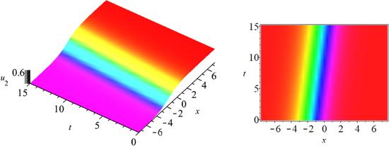
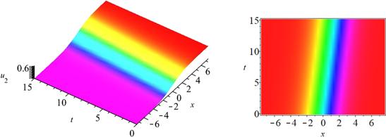
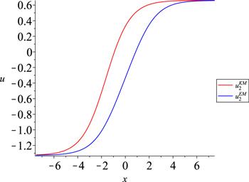
Figure 2 gives the dynamical features of the kink soliton ${u}_{2}\left(x,t\right)$ for ${a}_{1}=-1,$ ${b}_{0}=1,$ ${b}_{2}=1,$ ${c}_{1}=0.15,$ ${c}_{2}=0.15,$ and $a=2.7.$ Furthermore, the physical behaviors of ${u}_{2}^{{\rm{K}}{\rm{M}}}$ and ${u}_{2}^{{\rm{E}}{\rm{M}}}$ for above parameters have been given in figure 3 when $t=0.$

According to the authors’ knowledge, the outcomes of the current investigation are new and have been listed for the first time.

The authors successfully used a symbolic computation system to check the correctness of the outcomes of the current paper.

Figure 2. The kink soliton ${u}_{2}\left(x,t\right)$ for ${a}_{1}=-1,$ ${b}_{0}=1,$ ${b}_{2}=1,$ ${c}_{1}=0.15,$ ${c}_{2}=0.15,$ and $a=2.7.$
Figure 3. ${u}_{2}^{{\rm{K}}{\rm{M}}}$ and ${u}_{2}^{{\rm{E}}{\rm{M}}}$ for above parameters when $t=0.$

5. Conclusion

The principal aim of the current paper was to explore a newly well-established model known as the Sharma–Tasso–Olver–Burgers equation and derive its conservation laws and kink solitons. The study proceeded systematically by constructing the formal Lagrangian, Lie symmetries, and adjoint equations of STOBE to acquire its conservation laws. Besides, kink solitons of the STOBE were formally established using Kudryashov and exponential methods. Various plots in 2 and 3D postures were graphically represented to observe the dynamical characteristics of kink solitons. Based on information from the authors, the outcomes of the current investigation are new and have been listed for the first time. The authors’ suggestion for future works is employing newly well-organized methods [3844] to acquire other wave structures of STOBE.

Declaration of competing interest

The authors declare no conflict of interest.
1
Xie F Yan Z Zhang H 2001 Explicit and exact traveling wave solutions of Whitham–Broer–Kaup shallow water equations Phys. Lett. A 285 76 80

DOI

2
Bai C 2001 Exact solutions for nonlinear partial differential equation: a new approach Phys. Lett. A 288 191 195

DOI

3
Seadawy A R Kumar D Hosseini K Samadani F 2018 The system of equations for the ion sound and Langmuir waves and its new exact solutions Results Phys. 9 1631 1634

DOI

4
Rezazadeh H Kumar D Sulaiman T A Bulut H 2019 New complex hyperbolic and trigonometric solutions for the generalized conformable fractional Gardner equation Modern Phys. Lett. B 33 1950196

DOI

5
Ma H C Zhang Z P Deng A P 2012 A new periodic solution to Jacobi elliptic functions of MKdV equation and BBM equation Acta Math. Appl. Sin. 28 409 415

DOI

6
El-Sheikh M M A Seadawy A R Ahmed H M Arnous A H Rabie W B 2020 Dispersive and propagation of shallow water waves as a higher order nonlinear Boussinesq-like dynamical wave equations Physica A 537 122662

DOI

7
Hosseini K Mirzazadeh M Vahidi J Asghari R 2020 Optical wave structures to the Fokas–Lenells equation Optik 207 164450

DOI

8
Hosseini K Salahshour S Mirzazadeh M Ahmadian A Baleanu D Khoshrang A 2021 The (2 + 1)-dimensional Heisenberg ferromagnetic spin chain equation: its solitons and Jacobi elliptic function solutions Eur. Phys. J. Plus 136 206

DOI

9
Kudryashov N A 2012 One method for finding exact solutions of nonlinear differential equations Commun. Nonlinear Sci. Numer. Simul. 17 2248 2253

10
Ege S M Misirli E 2014 The modified Kudryashov method for solving some fractional-order nonlinear equations Adv. Differ. Equ. 2014 135

DOI

11
Hosseini K Bekir A Kaplan M 2017 New exact traveling wave solutions of the Tzitzéica-type evolution equations arising in non-linear optics J. Mod. Opt. 64 1688 1692

12
Kumar D Seadawy A R Joardar A K 2018 Modified Kudryashov method via new exact solutions for some conformable fractional differential equations arising in mathematical biology Chin. J. Phys. 56 75 85

13
Kumar D Darvishi M T Joardar A K 2018 Modified Kudryashov method and its application to the fractional version of the variety of Boussinesq-like equations in shallow water Opt. Quantum Electron. 50 128

14
Hosseini K Korkmaz A Bekir A Samadani F Zabihi A Topsakal M 2021 New wave form solutions of nonlinear conformable time-fractional Zoomeron equation in (2+1)-dimensions Waves Random Complex Media 31 228 238

DOI

15
He J H Wu X H 2006 Exp-function method for nonlinear wave equations Chaos Solitons Fractals 30 700 708

DOI

16
Ali A T Hassan E R 2010 General expa function method for nonlinear evolution equations Appl. Math. Comput. 217 451 459

DOI

17
Hosseini K Mirzazadeh M Zhou Q Liu Y Moradi M 2019 Analytic study on chirped optical solitons in nonlinear metamaterials with higher order effects Laser Phys. 29 095402

DOI

18
Hosseini K Osman M S Mirzazadeh M Rabiei F 2020 Investigation of different wave structures to the generalized third-order nonlinear Scrödinger equation Optik 206 164259

DOI

19
Hosseini K Mirzazadeh M Rabiei F Baskonus H M Yel G 2020 Dark optical solitons to the Biswas–Arshed equation with high order dispersions and absence of self-phase modulation Optik 209 164576

DOI

20
Hosseini K Ansari R Zabihi A Shafaroody A Mirzazadeh M 2020 Optical solitons and modulation instability of the resonant nonlinear Schrӧdinger equations in (3 + 1)-dimensions Optik 209 164584

DOI

21
Yaşar E 2010 On the conservation laws and invariant solutions of the mKdV equation J. Math. Anal. Appl. 363 174 181

DOI

22
Olver P J 1993 Application of Lie Groups to Differential Equations New York Springer

23
Naz R Mahomed F M Mason D P 2008 Comparison of different approaches to conservation laws for some partial differential equations in fluid mechanics Appl. Math. Comput. 205 212 230

DOI

24
Celik N Seadawy A R Ozkan Y S Yasar E 2021 A model of solitary waves in a nonlinear elastic circular rod: abundant different type exact solutions and conservation laws Chaos Solitons Fractals 143 110486

DOI

25
Wang G Kara A H Fakhar K Vega-Guzmand J Biswas A 2016 Group analysis, exact solutions and conservation laws of a generalized fifth order KdV equation Chaos Solitons Fractals 86 8 15

DOI

26
Ibragimov N H Khamitova R Avdonina E D Galiakberova L R 2015 Conservation laws and solutions of a quantum drift-diffusion model for semiconductors Int. J. Non Linear Mech. 77 69 73

DOI

27
Ibragimov N H Kolsrud T 2004 Lagrangian approach to evolution equations: symmetries and conservation laws Nonlinear Dyn. 36 29 40

DOI

28
Akbulut A Taşcan F 2017 Lie symmetries, symmetry reductions and conservation laws of time fractional modified Korteweg–de Vries (mkdv) equation Chaos, Solitons Fractals 100 1 6

DOI

29
Ibragimov N H 2007 A new conservation theorem J. Math. Anal. Appl. 333 311 328

DOI

30
Yan Z Lou S 2020 Soliton molecules in Sharma–Tasso–Olver–Burgers equation Appl. Math. Lett. 104 106271

DOI

31
Or-Roshid H Rashidi M M 2017 Multi-soliton fusion phenomenon of Burgers equation and fission, fusion phenomenon of Sharma–Tasso–Olver equation J. Ocean Eng. Sci. 2 120 126

DOI

32
Wazwaz A M 2019 Multiple complex soliton solutions for the integrable KdV, fifth-order Lax, modified KdV, Burgers, and Sharma–Tasso–Olver equations Chin. J. Phys. 59 372 378

DOI

33
Hu X Miao Z Lin S 2021 Solitons molecules, lump and interaction solutions to a (2 + 1)-dimensional Sharma–Tasso–Olver–Burgers equation Chin. J. Phys. 74 175 183

DOI

34
Hosseini K Samadani F Kumar D Faridi M 2018 New optical solitons of cubic-quartic nonlinear Schrödinger equation Optik 157 1101 1105

35
Hosseini K Zabihi A Samadani F Ansari R 2018 New explicit exact solutions of the unstable nonlinear Schrödinger’s equation using the expa and hyperbolic function methods Opt. Quantum Electron. 50 82

DOI

36
Akbulut A Taşcan F 2018 On symmetries, conservation laws and exact solutions of the nonlinear Schrödinger–Hirota equation Waves Random Complex Media 28 389 398

DOI

37
Akbulut A Taşcan F 2017 Application of conservation theorem and modified extended tanh-function method to (1 + 1)-dimensional nonlinear coupled Klein–Gordon–Zakharov equation Chaos Solitons Fractals 104 33 40

DOI

38
Kaabar M K A Kaplan M Siri Z 2021 New exact soliton solutions of the (3 + 1)-dimensional conformable Wazwaz–Benjamin–Bona–Mahony equation via two novel techniques J. Funct. Spaces 2021 4659905

DOI

39
Kaabar M K A Martínez F Gómez‐Aguilar J F Ghanbari B Kaplan M Günerhan H 2021 New approximate analytical solutions for the nonlinear fractional Schrödinger equation with second‐order spatio‐temporal dispersion via double Laplace transform method Math. Methods Appl. Sci. 44 11138 11156

DOI

40
Zada L Nawaz R Nisar K S Tahir M Yavuz M Kaabar M K A Martínez F 2021 New approximate-analytical solutions to partial differential equations via auxiliary function method Partial Differ. Equ. Appl. Math. 4 100045

DOI

41
Bi Y Zhang Z Liu Q Liu T 2021 Research on nonlinear waves of blood flow in arterial vessels Commun. Nonlinear Sci. Numer. Simul. 102 105918

DOI

42
Roshid H O Noor N F M Khatun M S Baskonus H M Belgacem F B M 2021 Breather, multi-shock waves and localized excitation structure solutions to the extended BKP–Boussinesq equation Commun. Nonlinear Sci. Numer. Simul. 101 105867

DOI

43
Gao W Yel G Baskonus H M Cattani C 2020 Complex solitons in the conformable (2 + 1)-dimensional Ablowitz–Kaup–Newell–Segur equation AIMS Math. 5 507 521

DOI

44
Kumar A Ilhan E Ciancio A Yel G Baskonus H M 2021 Extractions of some new travelling wave solutions to the conformable Date-Jimbo-Kashiwara-Miwa equation AIMS Math. 6 4238 4264

DOI

Outlines

/