


1. Introduction
Solitons have been a focus of nonlinear research [1–4]. Nonlocal nonlinear media have also attracted the attention of many researchers due to their unique properties, such as strengthening the stability of nonlinear modes, prevent their collapse in a high-dimensional system [5, 6], suppress the modulational instability [7], and allow for the existence of bound states [8, 9]. Nonlocal nonlinear media is prevalent in nematic liquid crystal [10], lead glass [11], atomic vapor [12], and so on.
In nonlocal optical media, the refractive index of a certain point is not only related to the beam intensity of this point, but also to a certain range around the point. In 1997, the Snyder–Mitchell (SM) model was presented in a strongly nonlocal medium, and the accessible solitons were found [13]. Thereafter, its exact bright and dark solitons in one-dimensional weak nonlocal media [14] was found. An exact analytical solution of the SM model was obtained by Q. Guo in 2004, the large phase shift of solitons was found [15], and the abundant evolution results were revealed by experimental and theoretical calculations [16–18]. In addition, some studies show the interesting interaction in the nonlocal Kerr media [19–21]. At present, multiple solitons [22], ring vortex solitons [23], Laguerre and Hermite soliton clusters [24–27], gap solitons [28], Ince–Gaussian beams [29], Bessel–Gaussian solitons [30], and rogue waves [31] have also been found.
In recent years, the competing nonlocal nonlinear system has attracted a lot of attention. The competing nonlinearity system is the nonlinear response of the different physical processes acting together on the medium [32, 33]. In 2006, a one-dimensional phenomenological model with competing cubic and quintic (CCQ) nonlinearities [34] was proposed in a nonlocal medium. It could approximately be used to describe the propagation of light beam in nonlocal medium with a saturation of nonlinearity [35]. A large number of studies indicate that competing nonlocal nonlinearity can stabilize multiple solitons, such as a vortex with a topological number greater than 2, 1D multipole soliton, and bright and dark solitons [12]. Meanwhile, the interaction of solitons has been studied extensively [35–39]. Shen et al demonstrated that two branches of vortex solitons in the competing nonlocal nonlinear media can be stabilized [40]. Hu et al. found that the degree of nonlocality of nematic liquid crystal can be modulated by changing the bias voltage [41]. Ye et al found that soliton interactions could be controlled by adjusting the nonlocality and nonlinearity of the media [42]. And vortex solitons have also been found in the 2D nonlocal CCQ model [43]. There are no reports about multipole solitons in nonlocal CCQ media yet; therefore, their characteristic and stability in nonlocal CCQ media is worth studying further.
In this paper, firstly, we introduce the two-dimensional nonlocal CCQ model. Then, using the Newton conjugate gradient method (NCGM), novel dipole and quadrupole solitons and their rotating modes are found. We also discuss their stability by linear stability analysis and the propagation after introducing the initial random perturbation. By adjusting the propagation constant and the coefficients of cubic and quintic nonlinear terms, stable intervals can be found. For dipole solitons, stability can be controlled by the propagation constant and the quintic nonlinear coefficient. While for quadrupole solitons, the stability is mainly controlled by the propagation constant and the cubic nonlinear coefficient.
The rest of the paper is outlined as follows. Section 2 introduces the theory model under investigation. Section 3 explores several nonlinear modes and their stability. The final section (section 4 ) comprises a discussion and summary of the main results.
2. Model
We consider the propagation of optical beam in nonlocal media with nonlocal cubic and quintic nonlinearity described by the normalized nonlocal nonlinear Schrödinger equation [44]
$\begin{eqnarray}{\rm{i}}\displaystyle \frac{\partial {\rm{\Psi }}}{\partial z}+\left(\displaystyle \frac{{\partial }^{2}}{\partial {x}^{2}}+\displaystyle \frac{{\partial }^{2}}{\partial {y}^{2}}\right){\rm{\Psi }}+n{\rm{\Psi }}=0,\end{eqnarray}$
where &PSgr;(r, z) is the slowly varying envelope, z stands for the distance of propagation, x and y represent the transverse coordinates, $\begin{eqnarray}\begin{array}{rcl}n & = & {a}_{3}{\displaystyle \int }_{-\infty }^{\infty }{\displaystyle \int }_{-\infty }^{\infty }{R}_{3}\left(x-{x}^{{\prime} },y-{y}^{{\prime} }\right)\\ & & \times \,| {\rm{\Psi }}\left({x}^{{\prime} },{y}^{{\prime} },z\right){| }^{2}{\rm{d}}{x}^{{\prime} }{\rm{d}}{y}^{{\prime} }\\ & & +\,{a}_{5}{\displaystyle \int }_{-\infty }^{\infty }{\displaystyle \int }_{-\infty }^{\infty }{R}_{5}\left(x-{x}^{{\prime} },y-{y}^{{\prime} }\right)\\ & & \times \,| {\rm{\Psi }}\left({x}^{{\prime} },{y}^{{\prime} },z\right){| }^{4}{\rm{d}}{x}^{{\prime} }{\rm{d}}{y}^{{\prime} },\end{array}\end{eqnarray}$
represents the nonlinear refractive index, which changes with the light intensity. Here, a3 and a5, respectively, represent the strength of cubic and quintic nonlinearity, and the positive (negative) value of aj represents the self-focusing (self-defocusing) nonlinear effect. a3a5 > 0 represents the double nonlinearity provided by a single physical process; conversely, a3a5 < 0 represents the nonlinearity of the competition, which corresponds to the nonlinearity originated from two different processes [43].In this paper, we take the Gaussian form nonlocal response function ${R}_{i}(x,y)=\tfrac{1}{\sqrt{\pi }{\sigma }_{i}}$ exp $\left(-\tfrac{{x}^{2}+{y}^{2}}{{\sigma }_{i}^{2}}\right),\,(i=3,5)$ [32], and it satisfies the normalization condition ∫∫Ri(x, y)dxdy = 1, where the coefficient σi represents the range of nonlocality. σi → ∞ corresponds to a strongly nonlocal medium. σi → 0 corresponds to local medium or the δ-type response function. In the case of σi → 0, equations (1 ) and (2 ) are reduced into the cubic and quintic nonlinear Schrödinger equation ${\rm{i}}\tfrac{\partial {\rm{\Psi }}}{\partial z}$+$\left(\tfrac{{\partial }^{2}}{\partial {x}^{2}}+\tfrac{{\partial }^{2}}{\partial {y}^{2}}\right){\rm{\Psi }}+{a}_{3}| {\rm{\Psi }}{| }^{2}{\rm{\Psi }}+{a}_{5}| {\rm{\Psi }}{| }^{4}{\rm{\Psi }}=0.$
3. Soliton in competing nonlocal nonlinear media
In this section, we find the soliton solutions of equation (1 ), and discuss their stability. Assuming &PSgr; = ψ(x, y)eiμz, μ is the propagation constant, equations (1 ) and (2 ) become5 ) into equations (3 ) and (4 ), we can obtain a set of linear equations6 ) can be solved by using the Fourier collocation method [45]; if the real parts of the eigenvalues are Re(λ) ≥ 0, then the soliton is stable. Their stability is also proved by the split-step Fourier propagation method.
$\begin{eqnarray}-\mu \psi +\left(\displaystyle \frac{{\partial }^{2}}{\partial {x}^{2}}+\displaystyle \frac{{\partial }^{2}}{\partial {y}^{2}}\right)\psi +n\psi =0,\end{eqnarray}$
$\begin{eqnarray}\begin{array}{rcl}n & = & {a}_{3}{\displaystyle \int }_{-\infty }^{\infty }{\displaystyle \int }_{-\infty }^{\infty }{R}_{3}\left(x-{x}^{{\prime} },y-{y}^{{\prime} }\right)| \psi {| }^{2}{\rm{d}}{x}^{{\prime} }{\rm{d}}{y}^{{\prime} }\\ & & +\,{a}_{5}{\displaystyle \int }_{-\infty }^{\infty }{\displaystyle \int }_{-\infty }^{\infty }{R}_{5}\left(x-{x}^{{\prime} },y-{y}^{{\prime} }\right)| \psi {| }^{4}{\rm{d}}{x}^{{\prime} }{\rm{d}}{y}^{{\prime} }.\end{array}\end{eqnarray}$
By using NCGM, we can find their soliton solutions. Then, its linear stability can be analyzed by solving the linear stability spectrum of the solitary wave as follows. The soliton solution is perturbed by normal modes as $\begin{eqnarray}\begin{array}{rcl}{\rm{\Psi }}(x,y,z) & = & [\psi (x,y)+u(x,y){{\rm{e}}}^{-\lambda z}\\ & & +\,{v}^{* }(x,y){{\rm{e}}}^{-{\lambda }^{* }z}]{{\rm{e}}}^{{\rm{i}}\mu z},\end{array}\end{eqnarray}$
where u(x, y), v(x, y) ≪ 1 are normal-mode perturbations, and λ is the eigenvalue of this normal mode. Substituting equation ( $\begin{eqnarray}\begin{array}{rcl}{\rm{i}}\lambda u & = & -\mu u+{{\rm{\nabla }}}_{\perp }^{2}u+{nu}+({n}_{1}+{n}_{2})\psi ,\\ {\rm{i}}\lambda v & = & \mu v-{{\rm{\nabla }}}_{\perp }^{2}v-{nv}-({n}_{1}+{n}_{2}){\psi }^{* },\\ {n}_{1} & = & {\displaystyle \int }_{-\infty }^{\infty }{\displaystyle \int }_{-\infty }^{\infty }{R}_{3}\left(x-{x}^{{\prime} },y-{y}^{{\prime} }\right)\\ & & \times \,(\psi v+{\psi }^{* }u){\rm{d}}{x}^{{\prime} }{\rm{d}}{y}^{{\prime} },\\ {n}_{2} & = & {\displaystyle \int }_{-\infty }^{\infty }{\displaystyle \int }_{-\infty }^{\infty }{R}_{5}\left(x-{x}^{{\prime} },y-{y}^{{\prime} }\right)\\ & & \times \,2| \psi {| }^{2}(\psi v+{\psi }^{* }u){\rm{d}}{x}^{{\prime} }{\rm{d}}{y}^{{\prime} }.\end{array}\end{eqnarray}$
The eigenvalue problem equation (Using NCGM, we first find the nonlinear steady states of equation (3 ), then perform the linear stability analysis by equation (6 ) and study the propagations of the obtained steady states by numerically solving equations (1 ) and (2 ). The dipole solitons with σ3 = 5.5 and σ5 = 0.1 are shown in figure 1. Figure 1(a) shows the profile of a dipole soliton when μ = 0.28. With the increase of propagation constant μ, the profile of dipole solitons will change. Their cross sections are plotted by taking y = 0 in figure 1(b). We find that the width will increase with the propagation constant, so the power P = ∫∫∣&PSgr;∣2dxdy also increases as shown in figure 1(c). The power curve not only shows us the change in the profile with the propagation constant, but also provides the range of the existence of dipole solitons. To check the stability of dipole solitons, the eigenvalue problem equation (6 ) is solved, and the results are plotted in figure 1(d). From this, the stable interval of dipole solitons that changed with the propagation constant are found. When the value of μ is small, the real part of eigenvalue Re (λ) is close to zero, which means that these dipole solitons can propagate stably. With the increase of μ, the solitons become unstable.
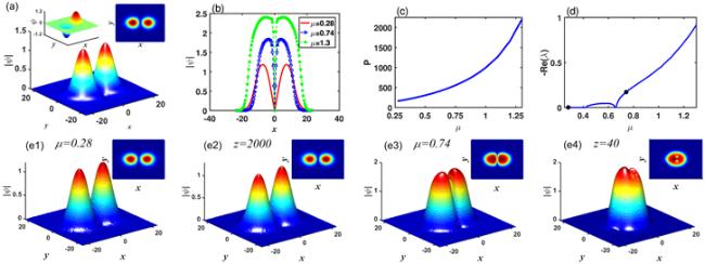
Figure 1. (a) Profile of the dipole soliton. (b) Cross section of the dipole soliton with different propagation constant μ. (c), (d) Power and stability curves of dipole solitons as a function of propagation constant μ. (e1)–(e4) The initial profiles of the dipole solitons with perturbation and their propagation results for μ = 0.28 and 0.74, respectively. The insets illustrate the projections of their profiles. Here, a3 = 1, a5 = −0.1, σ3 = 5.5, and σ5 = 0.1. |
The stability is proved further by a numerical propagation of equations (1 ) and (2 ), and adding random perturbations into the initial value of propagation, i.e., the initial value is taken as &PSgr;(x, y, 0) = ψ(x, y)(1 + ερ), where ε = 0.01 and ρ is the random variable uniformly distributed in the interval [0, 1]. We choose two dipole solitons with μ = 0.28 and 0.74 to propagate. The results of their stability correspond to the two points in figure 1(d). The propagation results and their projections are shown in figures 1(e1)–(e4). From them, these results are propagated and the linear stability analysis shown in figure 1(d) agree very well.
The effect of the cubic nonlinear coefficient σ3 on the properties of dipole solitons is shown in figure 2, where μ = 0.5. In figure 2(a), the cross sections of dipole solitons by taking y = 0 are shown with the different σ3. Figures 2(b) and (c) illustrate power and stability curves as a function of the cubic nonlinear coefficient σ3. From the stability curves, the cubic nonlinearity σ3 is unfavorable for the stability of dipole solitons. The two points in figure 2(c) represent the stability results of solitons with σ3 = 4.5 and 5, respectively. Figures 2(d1)–(d4) show the initial profiles and their propagation results. The stable dipole soliton in figure 2(d1) can conserve the profile after propagating z = 1000 from figure 2(d2), but the unstable one in figure 2(d3) is deformation after propagating z = 150 as shown in figure 2(d4). From these, the cubic nonlinearity can also be used to stabilize dipole solitons.
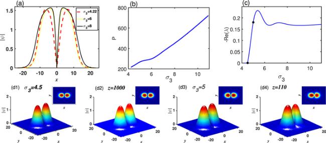
Figure 2. (a) Cross section of the dipole soliton with different cubic nonlinear coefficient σ5. (b), (c) Power and stability curves of dipole solitons as a function of the cubic nonlinear coefficient σ3. (d1)–(d4) The initial profiles of the dipole solitons with perturbation and their propagation results for σ3 = 4.5 and 5, respectively. The insets illustrate the projections of their profiles. Here, μ = 0.5, a3 = 1, a5 = −0.1, and σ5 = 0.1. |
The effect of the quintic nonlinear coefficient σ5 on the properties of dipole solitons is shown in figure 3, where μ = 0.5. In figure 3(a), the cross sections of dipole solitons by taking y = 0 are shown with the different σ5. The width of the profiles become narrow with the increase of σ5. Figures 3(b) and (c) illustrate the power and stability curves as a function of the quintic nonlinear coefficient σ5. From the power and stability curves, one can find that though there exists a dipole soliton when σ5 = 0, the quintic nonlinearity can stabilize dipole solitons when σ5 ∈ [2.75, 9.8]. The two points in figure 3(c) represent the stability results of solitons with σ5 = 0.1 and 2.93, respectively. Figure 3(d1) shows the initial profile of the dipole solitons with σ5 = 0.1. Figure 3(d2) shows the profile after propagating z = 90, which is obviously deformed. However, figures 3(d3)–(d4) show the initial profiles with σ5 = 2.93 and the propagation results with z = 3000. This shows that adjusting σ5 can stabilize dipole solitons. From figures 3(c) and (d1)–(d4), the quintic nonlinear coefficient σ5 is also very important in stabilizing dipole solitons.
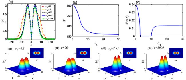
Figure 3. (a) Cross section of the dipole soliton with different quintic nonlinear coefficient σ5. (b), (c) Power and stability curves of dipole solitons as a function of the quintic nonlinear coefficient σ5. (d1)–(d4) The initial profiles of the dipole solitons with perturbation and their propagation results for σ5 = 0.1 and 2.93, respectively. The insets illustrate the projections of their profiles. Here, μ = 0.5, a3 = 1, a5 = −0.1, and σ3 = 5.5. |
We also find other types of dipole solitons that are symmetric along the diagonals, which we call rotation dipole solitons, as shown in figures 4–6. Because the rotation dipole solitons are similar to the counterclockwise rotation of solitons in figures 1–3. These solitons have properties similar to those shown in figures 1–3.
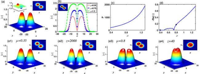
Figure 4. (a) Profile of the rotation dipole soliton. (b) Cross section along the dotted black line of the dipole soliton with different propagation constant μ. (c), (d) Power and stability curves of dipole solitons as a function of propagation constant μ. (e1)–(e4) The initial profiles of the dipole solitons with perturbation and their propagation results for μ = 0.35 and 0.8, respectively. The insets illustrate the projections of their profiles. Here, a3 = 1, a5 = −0.1, σ3 = 5.0, and σ5 = 0.1. |
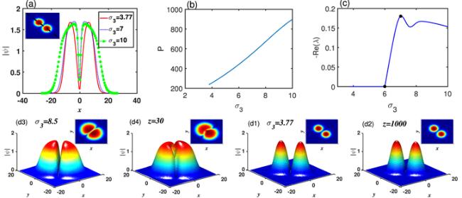
Figure 5. (a) Cross section of the rotation dipole soliton with different cubic nonlinear coefficient σ3. (b), (c) Power and stability curves of dipole solitons as a function of the cubic nonlinear coefficient σ3. (d1)–(d4) The initial profiles of the dipole solitons with perturbation and their propagation results for σ3 = 3.77 and 8.5, respectively. The insets illustrate the projections of their profiles. Here, μ = 0.6, a3 = 1, a5 = −0.1, σ5 = 0.1. |
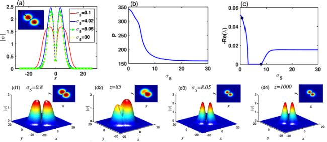
Figure 6. (a) Cross section of the rotation dipole soliton with different quintic nonlinear coefficient σ5. (b), (c) Power and stability curves of the dipole solitons as a function of the quintic nonlinear coefficient σ5. (d1)–(d4) The initial profiles of the dipole solitons with perturbation and their propagation results for σ5 = 0.8 and 8.05, respectively. The insets illustrate the projections of their profiles. Here, μ = 0.6, a3 = 1, a5 = −0.1, and σ3 = 5.0. |
Furthermore, the quadrupole solitons shown in figures 7–9 are found. In figures 7(a) and (b), a profile of the quadrupole soliton and the cross sections with different propagation constant are shown. Figures 7(c) and (d) illustrate power and stability curves as a function of the propagation constant. Though the stable region of quadrupole solitons is narrow, these solitons in the stable interval are stable. Through the propagation results shown in figures 7(e1)–(e4), we find that the unstable quadrupole soliton shown in figure 7(e1) is severely deformed after propagating z = 20 as shown in figure 7(e2), but the stable one in figure 7(e3) can conserve the profile even after propagating z = 140 from figure 7(e4). It is obvious that the propagation constant can be used to stabilize quadrupole solitons.
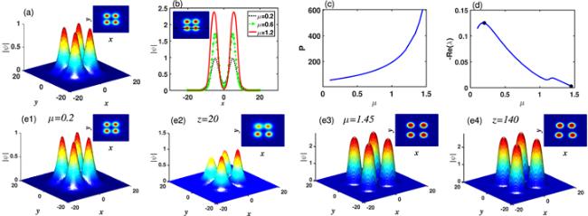
Figure 7. (a) Profile of the quadrupole soliton. (b) Cross section of the quadrupole soliton with different propagation constant μ. (c), (d) Power and stability curves of the quadrupole soliton as a function of the propagation constant μ. (e1)–(e4) The initial profiles of the quadrupole solitons with perturbation and their propagation results for μ = 0.2 and 1.45, respectively. The insets illustrate the projections of their profiles. Here, a3 = 1, a5 = −0.1, σ3 = 1.0, and σ5 = 0.1. |
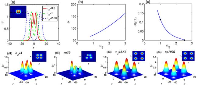
Figure 8. (a) Cross section of the quadrupole soliton with different cubic nonlinear coefficient σ3. (b), (c) Power and stability curves of the quadrupole solitons as a function of the cubic nonlinear coefficient σ3. (d1)–(d4) The initial profiles of the quadrupole solitons with perturbation and their propagation results for σ3 = 1 and 2.53, respectively. The insets illustrate the projections of their profiles. Here, μ = 0.3, a3 = 1, a5 = −0.1, and σ5 = 0.1. |
In figures 8(a)–(c), the cross section of the quadrupole soliton profile with different cubic nonlinear coefficients, and the power and stability curves as a function of σ3 are displayed. From the result of the stability analysis shown in figure 8(c), cubic nonlinearity is favorable for the stability of quadrupole solitons. Figures 8(d1)–(d4) show the initial profiles and their propagation results with different cubic nonlinearity. The unstable quadrupole soliton shown in figure 8(d1) with σ3 = 1 is deformation after propagating z = 30 as shown in figure 8(d2). The stable one in figure 8(d3) can conserve the profile after propagating z = 1000 from figure 8(d4). Therefore, the cubic nonlinearity can be used to stabilize quadrupole solitons.
The effect of quintic nonlinearity on quadrupole solitons is shown in figure 9. From the result of the stability analysis shown in figure 9(c), quintic nonlinearity is unfavorable for the stability of quadrupole solitons. Of course, the quintic nonlinear coefficient σ5 also affects the stability curve, the value of −Re (λ) increases first from 0.125, then decreases, and eventually tends to be constant with the increase of σ5. The unstable conclusion is also proved by the propagation results in shown figures 9(d1)–(d4), and the profiles become deformed after propagating z = 10.
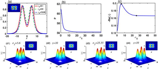
Figure 9. (a) Cross section of the quadrupole soliton with different quintic nonlinear coefficient σ5. (b), (c) Power and stability curves of quadrupole solitons as a function of the quintic nonlinear coefficient σ5. (d1)–(d4) The initial profiles of the quadrupole solitons with perturbation and their propagation results for σ5 = 5.6 and σ5 = 25.55, respectively. The insets illustrate the projections of their profiles. Here, μ = 0.18, a3 = 1, a5 = −0.1, and σ3 = 1.0. |
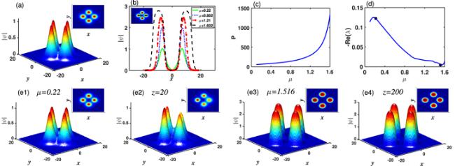
Figure 10. (a) Profile of the rotation quadrupole soliton. (b) Cross section of the quadrupole soliton along the dotted black line with different propagation constant μ. (c), (d) Power and stability curves of the quadrupole soliton as a function of propagation constant μ. (e1)–(e4) The initial profiles of the quadrupole solitons with perturbation and their propagation results for μ = 0.22 and 1.516, respectively. The insets illustrate the projections of their profiles. Here, a3 = 1, a5 = −0.1, σ3 = 1.0, and σ5 = 0.1. |
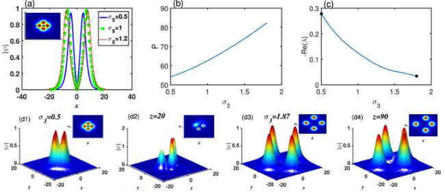
Figure 11. (a) Cross section of the rotation quadrupole soliton with different quintic nonlinear coefficient σ3. (b), (c) Power and stability curves of quadrupole solitons as a function of the quintic nonlinear coefficient σ3. (d1)–(d4) The initial profiles of the quadrupole solitons with perturbation and their propagation results for σ3 = 0.5 and 1.87, respectively. The insets illustrate the projections of their profiles. Here, μ = 0.2, a3 = 1, a5 = −0.1, and σ5 = 0.1. |
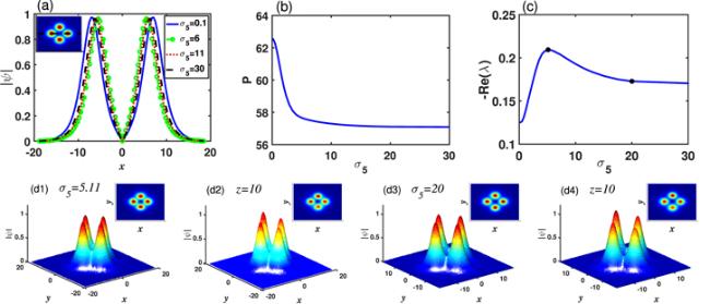
Figure 12. (a) Cross section of the rotation quadrupole soliton with different quintic nonlinear coefficient σ5. (b), (c) Power and stability curves of quadrupole solitons as a function of the quintic nonlinear coefficient σ5. (d1)–(d4) The initial profiles of the quadrupole solitons with perturbation and their propagation results for σ5 = 5.11 and 20, respectively. The insets illustrate the projections of their profiles. Here, μ = 0.2, a3 = 1, a5 = −0.1, and σ3 = 1.0. |
4. Conclusion and summary
In this paper, we have discussed a two-dimensional nonlocal model with competing self-focusing cubic and self-defocusing quintic nonlinearity. The dipole soliton, quadrupole soliton, and their rotation solitons were obtained. By linear stability analysis and numerical propagation, we found that the propagation constant could be used to stabilize them. We also discussed the effect of cubic nonlinearity and quintic nonlinearity on the stability, found that cubic nonlinearity could be used to stabilize dipole and quadrupole solitons, and quintic nonlinearity could be used to stabilize the dipole soliton. These numerical results would help the future experimental work on the nonlocal CCQ nonlinearity model.