Welcome to visit Communications in Theoretical Physics,
Particle Physics and Quantum Field Theory

Decay properties of the X(3872) through the Fierz rearrangement

  • Hua-Xing Chen
Expand
  • School of Physics, Southeast University, Nanjing 210094, China

Received date: 2021-11-06

  Revised date: 2021-12-09

  Accepted date: 2021-12-20

  Online published: 2022-03-10

Copyright

© 2022 Institute of Theoretical Physics CAS, Chinese Physical Society and IOP Publishing

Abstract

We systematically construct all the tetraquark currents of JPC = 1++ with the quark configurations $[{cq}][\bar{c}\bar{q}]$, $[\bar{c}q][\bar{q}c]$, and $[\bar{c}c][\bar{q}q]$ (q = u/d). Their relations are derived using the Fierz rearrangement of the Dirac and color indices, through which we study decay properties of the X(3872) under both the compact tetraquark and hadronic molecule interpretations. We conduct a search for the X(3872) → χc0π, ηcππ, and χc1ππ decay processes in particle experiments.

Cite this article

Hua-Xing Chen . Decay properties of the X(3872) through the Fierz rearrangement[J]. Communications in Theoretical Physics, 2022 , 74(2) : 025201 . DOI: 10.1088/1572-9494/ac449e

1. Introduction

Since the discovery of the X(3872) in 2003 by Belle [1], many charmonium-like XYZ states have been discovered in the past twenty years [2]. They are good candidates of four-quark states consisting of two quarks and two antiquarks, and their experimental and theoretical studies have significantly improved our understanding of the strong interaction at the low energy region. Although there is still a long way to go to fully understand how the strong interaction binds these quarks and antiquarks together with gluons, this subject has become and will continuously be one of the most intriguing research topics in hadron physics [310].
The X(3872) is the most puzzling state among all the charmonium-like XYZ states. Although it is denoted as the χc1(3872) in PDG2018 [2], the mass of the charmonium state χc1(2P) was estimated to be 3.95 GeV [11], significantly higher than the X(3872). This challenges the interpretation of the X(3872) as a conventional charmonium state, and various interpretations were proposed to explain it, such as a compact tetraquark state composed of a diquark and an antidiquark [1217], a loosely-bound hadronic molecular state composed of two charmed mesons [1824], and a hybrid charmonium state with constituents $c\bar{c}g$ [25, 26], etc. There were also some studies of the X(3872) as a conventional $c\bar{c}$ state [2730], and it was considered as the mixture of a $c\bar{c}$ state with a $D{\bar{D}}^{* }$ component in [3133]. We refer to reviews [310] for detailed discussions.
The charged charmonium-like state X(3872) of JPC = 1++ [34] has been observed in the ${D}^{0}{\bar{D}}^{* 0}$, J/ψππ, J/ψω, and γJ/ψ decay channels [3544], and there have been some evidences for the X(3872) → γψ(2S) decay [42, 44]. Especially, its decay channels J/ψππ and J/ψω have comparable branching ratios [3841], implying a large isospin violation. In a recent BESIII experiment [45], evidence for the X(3872) → χc1π decay was reported with a statistical significance of 5.2σ using data at center-of-mass energies between 4.15 and 4.30 GeV, while this was not confirmed in the later Belle experiment [46]. We refer to a recent paper [47], where the authors presented a complete analysis of all the existing experimental data and determine the absolute branching fractions of the X(3872) decays. We also refer to another recent paper [48], which studies branching fractions of the X(3872) from a theoretical point of view. There have been many experimental and theoretical studies on this subject, and we refer to reviews [310] for more discussions.
In [49] we studied decay properties of the Zc(3900) through the Fierz rearrangement of the Dirac and color indices, and in this paper we shall apply the same method to study decay properties of the X(3872). Both of these two studies are based on our previous finding that the diquark-antidiquark currents ($[{qq}][\bar{q}\bar{q}]$) and the meson-meson currents ($[\bar{q}q][\bar{q}q]$) are related to each other through the Fierz rearrangement of the Dirac and color indices [5053]. More studies on light baryon operators can be found in [54, 55]. The present study follows the idea of the QCD factorization method [5658], which has been widely and successfully applied to study weak decay properties of (heavy) hadrons.
The X(3872), as either a compact tetraquark state or a hadronic molecular state, contains four quarks. There can be three configurations (q = u/d):
$\begin{eqnarray*}[{cq}][\bar{c}\bar{q}],\,\,[\bar{c}q][\bar{q}c],\,\,\mathrm{and}\,\,[\bar{c}c][\bar{q}q].\end{eqnarray*}$
In this paper we shall apply the Fierz rearrangement to relate them, and extract some strong decay properties of the X(3872) under both the compact tetraquark and hadronic molecule interpretations. We shall not calculate the absolute values of these decay widths, but extract their relative branching ratios, which are also useful to understand the nature of the X(3872) [59]. A similar arrangement in the nonrelativistic case was used to study strong decay properties of the X(3872) and Zc(3900) in [6062].
This paper is organized as follows. In section 2 we systematically construct all the tetraquark currents of JPC = 1++ with the quark content $c\bar{c}q\bar{q}$. We consider three configurations, $[{cq}][\bar{c}\bar{q}]$, $[\bar{c}q][\bar{q}c]$, and $[\bar{c}c][\bar{q}q]$, and we derive their relations using the Fierz rearrangement of the Dirac and color indices. In section 3 and section 4 we extract some isoscalar decay channels of the X(3872), separately for the compact tetraquark and hadronic molecule interpretations, and in section 5 we investigate its isovector decay channels. The obtained results are discussed in section 6, and formulae of decay amplitudes and decay widths are given in appendix A.

2. Tetraquark currents of JPC = 1++ and their relations

Similar to [49], we can use the c, $\bar{c}$, q, $\bar{q}$ quarks (q = u/d) to construct three types of tetraquark currents of JPC = 1++, as illustrated in figure 1:
$\begin{eqnarray}\begin{array}{rcl}\eta (x,y) & = & [{q}_{a}^{{\rm{T}}}(x)\,{\mathbb{C}}{{\rm{\Gamma }}}_{1}\,{c}_{b}(x)]\times [{\bar{q}}_{c}(y)\,{{\rm{\Gamma }}}_{2}{\mathbb{C}}\,{\bar{c}}_{d}^{{\rm{T}}}(y)],\\ \xi (x,y) & = & [{\bar{c}}_{a}(x)\,{{\rm{\Gamma }}}_{3}\,{q}_{b}(x)]\times [{\bar{q}}_{c}(y)\,{{\rm{\Gamma }}}_{4}\,{c}_{d}(y)],\\ \theta (x,y) & = & [{\bar{c}}_{a}(x)\,{{\rm{\Gamma }}}_{5}\,{c}_{b}(x)]\times [{\bar{q}}_{c}(y)\,{{\rm{\Gamma }}}_{6}\,{q}_{d}(y)],\end{array}\end{eqnarray}$
where Γi are Dirac matrices, and the subscripts a, b, c, d are color indices. We separately construct them in the following subsections.
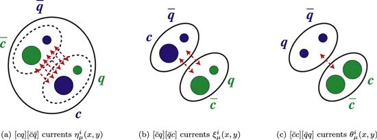
Figure 1. Three types of tetraquark currents. Quarks and antiquarks are shown in red, green, and blue color.
Generally speaking, one can apply the Fierz rearrangement to relate the local diquark-antidiquark currents η(x, x) and the local meson-meson currents ξ(x, x) and θ(x, x), but this equivalence is just between diquark-antidiquark and mesonic-mesonic currents, while compact diquark-antidiquark tetraquark states and weakly-bound meson-meson molecular states are totally different. To exactly describe them, one needs to explicitly use non-local currents to perform QCD sum rule analyses, but we are still not able to do this.

2.1. $[{qc}][\bar{q}\bar{c}]$ currents ${\eta }_{\mu }^{i}(x,y)$

There are eight independent $[{qc}][\bar{q}\bar{c}]$ currents of JPC = 1++ [63]:
$\begin{eqnarray}\begin{array}{rcl}{\eta }_{\mu }^{1} & = & {q}_{a}^{{\rm{T}}}{\mathbb{C}}{\gamma }_{\mu }{c}_{b}\,{\bar{q}}_{a}{\gamma }_{5}{\mathbb{C}}{\bar{c}}_{b}^{{\rm{T}}}+{q}_{a}^{{\rm{T}}}{\mathbb{C}}{\gamma }_{5}{c}_{b}\,{\bar{q}}_{a}{\gamma }_{\mu }{\mathbb{C}}{\bar{c}}_{b}^{{\rm{T}}},\\ {\eta }_{\mu }^{2} & = & {q}_{a}^{{\rm{T}}}{\mathbb{C}}{\gamma }_{\mu }{c}_{b}\,{\bar{q}}_{b}{\gamma }_{5}{\mathbb{C}}{\bar{c}}_{a}^{{\rm{T}}}+{q}_{a}^{{\rm{T}}}{\mathbb{C}}{\gamma }_{5}{c}_{b}\,{\bar{q}}_{b}{\gamma }_{\mu }{\mathbb{C}}{\bar{c}}_{a}^{{\rm{T}}},\\ {\eta }_{\mu }^{3} & = & {q}_{a}^{{\rm{T}}}{\mathbb{C}}{\gamma }^{\nu }{c}_{b}\,{\bar{q}}_{a}{\sigma }_{\mu \nu }{\gamma }_{5}{\mathbb{C}}{\bar{c}}_{b}^{{\rm{T}}}+{q}_{a}^{{\rm{T}}}{\mathbb{C}}{\sigma }_{\mu \nu }{\gamma }_{5}{c}_{b}\,{\bar{q}}_{a}{\gamma }^{\nu }{\mathbb{C}}{\bar{c}}_{b}^{{\rm{T}}},\\ {\eta }_{\mu }^{4} & = & {q}_{a}^{{\rm{T}}}{\mathbb{C}}{\gamma }^{\nu }{c}_{b}\,{\bar{q}}_{b}{\sigma }_{\mu \nu }{\gamma }_{5}{\mathbb{C}}{\bar{c}}_{a}^{{\rm{T}}}+{q}_{a}^{{\rm{T}}}{\mathbb{C}}{\sigma }_{\mu \nu }{\gamma }_{5}{c}_{b}\,{\bar{q}}_{b}{\gamma }^{\nu }{\mathbb{C}}{\bar{c}}_{a}^{{\rm{T}}},\\ {\eta }_{\mu }^{5} & = & {q}_{a}^{{\rm{T}}}{\mathbb{C}}{\gamma }_{\mu }{\gamma }_{5}{c}_{b}\,{\bar{q}}_{a}{\mathbb{C}}{\bar{c}}_{b}^{{\rm{T}}}+{q}_{a}^{{\rm{T}}}{\mathbb{C}}{c}_{b}\,{\bar{q}}_{a}{\gamma }_{\mu }{\gamma }_{5}{\mathbb{C}}{\bar{c}}_{b}^{{\rm{T}}},\\ {\eta }_{\mu }^{6} & = & {q}_{a}^{{\rm{T}}}{\mathbb{C}}{\gamma }_{\mu }{\gamma }_{5}{c}_{b}\,{\bar{q}}_{b}{\mathbb{C}}{\bar{c}}_{a}^{{\rm{T}}}+{q}_{a}^{{\rm{T}}}{\mathbb{C}}{c}_{b}\,{\bar{q}}_{b}{\gamma }_{\mu }{\gamma }_{5}{\mathbb{C}}{\bar{c}}_{a}^{{\rm{T}}},\\ {\eta }_{\mu }^{7} & = & {q}_{a}^{{\rm{T}}}{\mathbb{C}}{\gamma }^{\nu }{\gamma }_{5}{c}_{b}\,{\bar{q}}_{a}{\sigma }_{\mu \nu }{\mathbb{C}}{\bar{c}}_{b}^{{\rm{T}}}+{q}_{a}^{{\rm{T}}}{\mathbb{C}}{\sigma }_{\mu \nu }{c}_{b}\,{\bar{q}}_{a}{\gamma }^{\nu }{\gamma }_{5}{\mathbb{C}}{\bar{c}}_{b}^{{\rm{T}}},\\ {\eta }_{\mu }^{8} & = & {q}_{a}^{{\rm{T}}}{\mathbb{C}}{\gamma }^{\nu }{\gamma }_{5}{c}_{b}\,{\bar{q}}_{b}{\sigma }_{\mu \nu }{\mathbb{C}}{\bar{c}}_{a}^{{\rm{T}}}+{q}_{a}^{{\rm{T}}}{\mathbb{C}}{\sigma }_{\mu \nu }{c}_{b}\,{\bar{q}}_{b}{\gamma }^{\nu }{\gamma }_{5}{\mathbb{C}}{\bar{c}}_{a}^{{\rm{T}}}.\end{array}\end{eqnarray}$
In the above expressions we have omitted the coordinates x and y. The color structures of ${\eta }_{\mu }^{1}-{\eta }_{\mu }^{2}$, ${\eta }_{\mu }^{3}-{\eta }_{\mu }^{4}$, ${\eta }_{\mu }^{5}-{\eta }_{\mu }^{6}$, and ${\eta }_{\mu }^{7}-{\eta }_{\mu }^{8}$ are all antisymmetric ${[{qc}]}_{{\bar{{\bf{3}}}}_{c}}{[\bar{q}\bar{c}]}_{{{\bf{3}}}_{c}}\to {[{qc}\bar{q}\bar{c}]}_{{{\bf{1}}}_{c}}$, and those of ${\eta }_{\mu }^{1}+{\eta }_{\mu }^{2}$, ${\eta }_{\mu }^{3}+{\eta }_{\mu }^{4}$, ${\eta }_{\mu }^{5}+{\eta }_{\mu }^{6}$, and ${\eta }_{\mu }^{7}+{\eta }_{\mu }^{8}$ are all symmetric ${[{qc}]}_{{{\bf{6}}}_{c}}{[\bar{q}\bar{c}]}_{{\bar{{\bf{6}}}}_{c}}\to {[{qc}\bar{q}\bar{c}]}_{{{\bf{1}}}_{c}}$.
In the diquark-antidiquark model proposed in [12, 13, 64], the authors use $| {s}_{{qc}},{s}_{\bar{q}\bar{c}}{\rangle }_{J}$ to denote ground-state tetraquarks, where sqc and ${s}_{\bar{q}\bar{c}}$ are the charmed diquark and antidiquark spins, respectively. They interpret the X(3872) as a compact tetraquark state of JPC = 1++:
$\begin{eqnarray}| {0}_{{qc}}{1}_{\bar{q}\bar{c}};{1}^{++}\rangle =\displaystyle \frac{1}{\sqrt{2}}\left(| {0}_{{qc}},{1}_{\bar{q}\bar{c}}{\rangle }_{J=1}+| {1}_{{qc}},{0}_{\bar{q}\bar{c}}{\rangle }_{J=1}\right).\end{eqnarray}$
The interpolating current having the identical internal structure is the current ${\eta }_{\mu }^{1}-{\eta }_{\mu }^{2}$, which has been studied in [63, 6569]:
$\begin{eqnarray}\begin{array}{rcl}{\eta }_{\mu }^{{ \mathcal X }}(x,y) & = & {\eta }_{\mu }^{1}(x,y)-{\eta }_{\mu }^{2}(x,y)\\ & = & {q}_{a}^{{\rm{T}}}(x){\mathbb{C}}{\gamma }_{\mu }{c}_{b}(x)\left({\bar{q}}_{a}(y){\gamma }_{5}{\mathbb{C}}{\bar{c}}_{b}^{{\rm{T}}}(y)-\{a\leftrightarrow b\}\right)\\ & & +\{{\gamma }_{\mu }\leftrightarrow {\gamma }_{5}\}.\end{array}\end{eqnarray}$

2.2. $[\bar{c}q][\bar{q}c]$ currents ${\xi }_{\mu }^{i}(x,y)$

There are eight independent $[\bar{c}q][\bar{q}c]$ currents of JPC = 1++:
$\begin{eqnarray}\begin{array}{rcl}{\xi }_{\mu }^{1} & = & {\bar{c}}_{a}{\gamma }_{\mu }{q}_{a}\,{\bar{q}}_{b}{\gamma }_{5}{c}_{b}-{\bar{c}}_{a}{\gamma }_{5}{q}_{a}\,{\bar{q}}_{b}{\gamma }_{\mu }{c}_{b},\\ {\xi }_{\mu }^{2} & = & {\bar{c}}_{a}{\gamma }^{\nu }{q}_{a}\,{\bar{q}}_{b}{\sigma }_{\mu \nu }{\gamma }_{5}{c}_{b}+{\bar{c}}_{a}{\sigma }_{\mu \nu }{\gamma }_{5}{q}_{a}\,{\bar{q}}_{b}{\gamma }^{\nu }{c}_{b},\\ {\xi }_{\mu }^{3} & = & {\bar{c}}_{a}{\gamma }_{\mu }{\gamma }_{5}{q}_{a}\,{\bar{q}}_{b}{c}_{b}+{\bar{c}}_{a}{q}_{a}\,{\bar{q}}_{b}{\gamma }_{\mu }{\gamma }_{5}{c}_{b},\\ {\xi }_{\mu }^{4} & = & {\bar{c}}_{a}{\gamma }^{\nu }{\gamma }_{5}{q}_{a}\,{\bar{q}}_{b}{\sigma }_{\mu \nu }{c}_{b}-{\bar{c}}_{a}{\sigma }_{\mu \nu }{q}_{a}\,{\bar{q}}_{b}{\gamma }^{\nu }{\gamma }_{5}{c}_{b},\\ {\xi }_{\mu }^{5} & = & {\lambda }_{{ab}}^{n}{\lambda }_{{cd}}^{n}\times \left({\bar{c}}_{a}{\gamma }_{\mu }{q}_{b}\,{\bar{q}}_{c}{\gamma }_{5}{c}_{d}-{\bar{c}}_{a}{\gamma }_{5}{q}_{b}\,{\bar{q}}_{c}{\gamma }_{\mu }{c}_{d}\right),\\ {\xi }_{\mu }^{6} & = & {\lambda }_{{ab}}^{n}{\lambda }_{{cd}}^{n}\times \left({\bar{c}}_{a}{\gamma }^{\nu }{q}_{b}\,{\bar{q}}_{c}{\sigma }_{\mu \nu }{\gamma }_{5}{c}_{d}+{\bar{c}}_{a}{\sigma }_{\mu \nu }{\gamma }_{5}{q}_{b}\,{\bar{q}}_{c}{\gamma }^{\nu }{c}_{d}\right),\\ {\xi }_{\mu }^{7} & = & {\lambda }_{{ab}}^{n}{\lambda }_{{cd}}^{n}\times \left({\bar{c}}_{a}{\gamma }_{\mu }{\gamma }_{5}{q}_{b}\,{\bar{q}}_{c}{c}_{d}+{\bar{c}}_{a}{q}_{b}\,{\bar{q}}_{c}{\gamma }_{\mu }{\gamma }_{5}{c}_{d}\right),\\ {\xi }_{\mu }^{8} & = & {\lambda }_{{ab}}^{n}{\lambda }_{{cd}}^{n}\times \left({\bar{c}}_{a}{\gamma }^{\nu }{\gamma }_{5}{q}_{b}\,{\bar{q}}_{c}{\sigma }_{\mu \nu }{c}_{d}-{\bar{c}}_{a}{\sigma }_{\mu \nu }{q}_{b}\,{\bar{q}}_{c}{\gamma }^{\nu }{\gamma }_{5}{c}_{d}\right).\end{array}\end{eqnarray}$
The former four ${\xi }_{\mu }^{1,2,3,4}$ have the color structure ${[\bar{c}q]}_{{{\bf{1}}}_{c}}{[\bar{q}c]}_{{{\bf{1}}}_{c}}\to {[c\bar{c}q\bar{q}]}_{{{\bf{1}}}_{c}}$, and the latter four ${\xi }_{\mu }^{5,6,7,8}$ have thecolor structure ${[\bar{c}q]}_{{{\bf{8}}}_{c}}{[\bar{q}c]}_{{{\bf{8}}}_{c}}\to {[c\bar{c}q\bar{q}]}_{{{\bf{1}}}_{c}}$.
In the molecular picture the X(3872) is interpreted as the $D{\bar{D}}^{* }$ hadronic molecular state of JPC = 1++ [1824]:
$\begin{eqnarray}| D{\bar{D}}^{* };{1}^{++}\rangle =\displaystyle \frac{1}{\sqrt{2}}\left(| D{\bar{D}}^{* }{\rangle }_{J=1}+| \bar{D}{D}^{* }{\rangle }_{J=1}\right),\end{eqnarray}$
and the relevant interpolating current is just ${\xi }_{\mu }^{1}(x,y)$, which has been studied in [7073]:
$\begin{eqnarray}\begin{array}{l}{\xi }_{\mu }^{{ \mathcal X }}(x,y)={\xi }_{\mu }^{1}(x,y)\\ \quad ={\bar{c}}_{a}(x){\gamma }_{\mu }{q}_{a}(x)\,{\bar{q}}_{b}(y){\gamma }_{5}{c}_{b}(y)-\{{\gamma }_{\mu }\leftrightarrow {\gamma }_{5}\}.\end{array}\end{eqnarray}$

2.3. $[\bar{c}c][\bar{q}q]$ currents ${\theta }_{\mu }^{i}(x,y)$

There are eight independent $[\bar{c}c][\bar{q}q]$ currents of JPC = 1++:
$\begin{eqnarray}\begin{array}{rcl}{\theta }_{\mu }^{1}(x,y) & = & {\bar{c}}_{a}(x){c}_{a}(x)\,{\bar{q}}_{b}(y){\gamma }_{\mu }{\gamma }_{5}{q}_{b}(y),\\ {\theta }_{\mu }^{2}(x,y) & = & {\bar{c}}_{a}(x){\gamma }_{\mu }{\gamma }_{5}{c}_{a}(x)\,{\bar{q}}_{b}(y){q}_{b}(y),\\ {\theta }_{\mu }^{3}(x,y) & = & {\bar{c}}_{a}(x){\gamma }^{\nu }{c}_{a}(x)\,{\bar{q}}_{b}(y){\sigma }_{\mu \nu }{\gamma }_{5}{q}_{b}(y),\\ {\theta }_{\mu }^{4}(x,y) & = & {\bar{c}}_{a}(x){\sigma }_{\mu \nu }{\gamma }_{5}{c}_{a}(x)\,{\bar{q}}_{b}(y){\gamma }^{\nu }{q}_{b}(y),\\ {\theta }_{\mu }^{5}(x,y) & = & {\lambda }_{{ab}}^{n}{\lambda }_{{cd}}^{n}\times \left({\bar{c}}_{a}(x){c}_{b}(x)\,{\bar{q}}_{c}(y){\gamma }_{\mu }{\gamma }_{5}{q}_{d}(y)\right),\\ {\theta }_{\mu }^{6}(x,y) & = & {\lambda }_{{ab}}^{n}{\lambda }_{{cd}}^{n}\times \left({\bar{c}}_{a}(x){\gamma }_{\mu }{\gamma }_{5}{c}_{b}(x)\,{\bar{q}}_{c}(y){q}_{d}(y)\right),\\ {\theta }_{\mu }^{7}(x,y) & = & {\lambda }_{{ab}}^{n}{\lambda }_{{cd}}^{n}\times \left({\bar{c}}_{a}(x){\gamma }^{\nu }{c}_{b}(x)\,{\bar{q}}_{c}(y){\sigma }_{\mu \nu }{\gamma }_{5}{q}_{d}(y)\right),\\ {\theta }_{\mu }^{8}(x,y) & = & {\lambda }_{{ab}}^{n}{\lambda }_{{cd}}^{n}\times \left({\bar{c}}_{a}(x){\sigma }_{\mu \nu }{\gamma }_{5}{c}_{b}(x)\,{\bar{q}}_{c}(y){\gamma }^{\nu }{q}_{d}(y)\right).\end{array}\end{eqnarray}$
The former four ${\theta }_{\mu }^{1,2,3,4}$ have the color structure ${[\bar{c}c]}_{{{\bf{1}}}_{c}}{[\bar{q}q]}_{{{\bf{1}}}_{c}}\to {[c\bar{c}q\bar{q}]}_{{{\bf{1}}}_{c}}$, and the latter four ${\theta }_{\mu }^{5,6,7,8}$ havethe color structure ${[\bar{c}c]}_{{{\bf{8}}}_{c}}{[\bar{q}q]}_{{{\bf{8}}}_{c}}\to {[c\bar{c}q\bar{q}]}_{{{\bf{1}}}_{c}}$.

2.4. Fierz rearrangement

The Fierz rearrangement [74] of the Dirac and color indices has been systematically applied to study light baryon and tetraquark operators/currents in [4955]. All the necessary equations can be found in section 3.3.2 of [75]. More studies can be found in [69, 76]. In the present study we apply it to relate the above three types of tetraquark currents.
The Fierz rearrangement is usually applied to local operators/currents. However, it is actually a matrix identity, and is valid if the same quark field in the initial and final operators is at the same location. As an example, we can apply the Fierz rearrangement to transform the non-local current with the quark fields $\eta ({x}^{{\prime} },x;{y}^{{\prime} },y)=[q({x}^{{\prime} })c(x)][\bar{q}({y}^{{\prime} })\bar{c}(y)]$ into a combination of several non-local currents with the quark fields at same locations $\theta (y,x;{y}^{{\prime} },{x}^{{\prime} })=[\bar{c}(y)c(x)][\bar{q}({y}^{{\prime} })q({x}^{{\prime} })]$.
To apply it to study the decay process, we need to add two overall dynamical processes in the first and third steps:
$\begin{eqnarray}\begin{array}{rcl}\eta (x,y) & = & [q(x)\,c(x)]\,\times \,[\bar{q}(y)\,\bar{c}(y)]\\ \to \eta ({x}^{{\prime} },x;{y}^{{\prime} },y) & =\, & [q({x}^{{\prime} })\,c(x)]\,\times \,[\bar{q}({y}^{{\prime} })\,\bar{c}(y)]\\ \to \theta (y,x;{y}^{{\prime} },{x}^{{\prime} }) & =\, & [\bar{c}(y)\,c(x)]\,\times \,[\bar{q}({y}^{{\prime} })\,q({x}^{{\prime} })]\\ \to \theta ({x}^{{\prime\prime} };{y}^{{\prime\prime} }) & = & [\bar{c}({x}^{{\prime\prime} })\,c({x}^{{\prime\prime} })]\,+\,[\bar{q}({y}^{{\prime\prime} })\,q({y}^{{\prime\prime} })],\end{array}\end{eqnarray}$
which will be discussed in detail in the next section. The second step is the Fierz rearrangement whose explicit expressions are given as follows.
Altogether, we obtain the following relation between the currents ${\eta }_{\mu }^{i}({x}^{{\prime} },x;{y}^{{\prime} },y)$ and ${\theta }_{\mu }^{i}(y,x;{y}^{{\prime} },{x}^{{\prime} })$:
$\begin{eqnarray}\left(\begin{array}{c}{\eta }_{\mu }^{1}\\ {\eta }_{\mu }^{2}\\ {\eta }_{\mu }^{3}\\ {\eta }_{\mu }^{4}\\ {\eta }_{\mu }^{5}\\ {\eta }_{\mu }^{6}\\ {\eta }_{\mu }^{7}\\ {\eta }_{\mu }^{8}\end{array}\right)=\left(\begin{array}{cccccccc}-1/2 & 1/2 & -{\rm{i}}/2 & {\rm{i}}/2 & 0 & 0 & 0 & 0\\ -1/6 & 1/6 & -{\rm{i}}/6 & {\rm{i}}/6 & -1/4 & 1/4 & -{\rm{i}}/4 & {\rm{i}}/4\\ -3{\rm{i}}/2 & -3{\rm{i}}/2 & 1/2 & 1/2 & 0 & 0 & 0 & 0\\ -{\rm{i}}/2 & -{\rm{i}}/2 & 1/6 & 1/6 & -3{\rm{i}}/4 & -3{\rm{i}}/4 & 1/4 & 1/4\\ -1/2 & -1/2 & {\rm{i}}/2 & {\rm{i}}/2 & 0 & 0 & 0 & 0\\ -1/6 & -1/6 & {\rm{i}}/6 & {\rm{i}}/6 & -1/4 & -1/4 & {\rm{i}}/4 & {\rm{i}}/4\\ -3{\rm{i}}/2 & 3{\rm{i}}/2 & -1/2 & 1/2 & 0 & 0 & 0 & 0\\ -{\rm{i}}/2 & {\rm{i}}/2 & -1/6 & 1/6 & -3{\rm{i}}/4 & 3{\rm{i}}/4 & -1/4 & 1/4\end{array}\right)\times \left(\begin{array}{c}{\theta }_{\mu }^{1}\\ {\theta }_{\mu }^{2}\\ {\theta }_{\mu }^{3}\\ {\theta }_{\mu }^{4}\\ {\theta }_{\mu }^{5}\\ {\theta }_{\mu }^{6}\\ {\theta }_{\mu }^{7}\\ {\theta }_{\mu }^{8}\end{array}\right),\end{eqnarray}$
the following relation between ${\eta }_{\mu }^{i}({x}^{{\prime} },x;{y}^{{\prime} },y)$ and ${\xi }_{\mu }^{i}(y,{x}^{{\prime} };{y}^{{\prime} },x)$:
$\begin{eqnarray}\left(\begin{array}{c}{\eta }_{\mu }^{1}\\ {\eta }_{\mu }^{2}\\ {\eta }_{\mu }^{3}\\ {\eta }_{\mu }^{4}\\ {\eta }_{\mu }^{5}\\ {\eta }_{\mu }^{6}\\ {\eta }_{\mu }^{7}\\ {\eta }_{\mu }^{8}\end{array}\right)=\left(\begin{array}{cccccccc}1/6 & 0 & 0 & -{\rm{i}}/6 & 1/4 & 0 & 0 & -{\rm{i}}/4\\ 1/2 & 0 & 0 & -{\rm{i}}/2 & 0 & 0 & 0 & 0\\ 0 & -1/6 & {\rm{i}}/2 & 0 & 0 & -1/4 & 3{\rm{i}}/4 & 0\\ 0 & -1/2 & 3{\rm{i}}/2 & 0 & 0 & 0 & 0 & 0\\ 0 & {\rm{i}}/6 & -1/6 & 0 & 0 & {\rm{i}}/4 & -1/4 & 0\\ 0 & {\rm{i}}/2 & -1/2 & 0 & 0 & 0 & 0 & 0\\ -{\rm{i}}/2 & 0 & 0 & 1/6 & -3{\rm{i}}/4 & 0 & 0 & 1/4\\ -3{\rm{i}}/2 & 0 & 0 & 1/2 & 0 & 0 & 0 & 0\end{array}\right)\times \left(\begin{array}{c}{\xi }_{\mu }^{1}\\ {\xi }_{\mu }^{2}\\ {\xi }_{\mu }^{3}\\ {\xi }_{\mu }^{4}\\ {\xi }_{\mu }^{5}\\ {\xi }_{\mu }^{6}\\ {\xi }_{\mu }^{7}\\ {\xi }_{\mu }^{8}\end{array}\right),\end{eqnarray}$
the following relation among ${\eta }_{\mu }^{i}({x}^{{\prime} },x;{y}^{{\prime} },y)$, ${\xi }_{\mu }^{1,2,3,4}(y,{x}^{{\prime} };{y}^{{\prime} },x)$, and ${\theta }_{\mu }^{1,2,3,4}(y,x;{y}^{{\prime} },{x}^{{\prime} })$:
$\begin{eqnarray}\left(\begin{array}{c}{\eta }_{\mu }^{1}\\ {\eta }_{\mu }^{2}\\ {\eta }_{\mu }^{3}\\ {\eta }_{\mu }^{4}\\ {\eta }_{\mu }^{5}\\ {\eta }_{\mu }^{6}\\ {\eta }_{\mu }^{7}\\ {\eta }_{\mu }^{8}\end{array}\right)=\left(\begin{array}{cccccccc}0 & 0 & 0 & 0 & -1/2 & 1/2 & -{\rm{i}}/2 & {\rm{i}}/2\\ 1/2 & 0 & 0 & -{\rm{i}}/2 & 0 & 0 & 0 & 0\\ 0 & 0 & 0 & 0 & -3{\rm{i}}/2 & -3{\rm{i}}/2 & 1/2 & 1/2\\ 0 & -1/2 & 3{\rm{i}}/2 & 0 & 0 & 0 & 0 & 0\\ 0 & 0 & 0 & 0 & -1/2 & -1/2 & {\rm{i}}/2 & {\rm{i}}/2\\ 0 & {\rm{i}}/2 & -1/2 & 0 & 0 & 0 & 0 & 0\\ 0 & 0 & 0 & 0 & -3{\rm{i}}/2 & 3{\rm{i}}/2 & -1/2 & 1/2\\ -3{\rm{i}}/2 & 0 & 0 & 1/2 & 0 & 0 & 0 & 0\end{array}\right)\times \left(\begin{array}{c}{\xi }_{\mu }^{1}\\ {\xi }_{\mu }^{2}\\ {\xi }_{\mu }^{3}\\ {\xi }_{\mu }^{4}\\ {\theta }_{\mu }^{1}\\ {\theta }_{\mu }^{2}\\ {\theta }_{\mu }^{3}\\ {\theta }_{\mu }^{4}\end{array}\right),\end{eqnarray}$
and the following relation between ${\xi }_{\mu }^{i}(y,{x}^{{\prime} };{y}^{{\prime} },x)$ and ${\theta }_{\mu }^{i}(y,x;{y}^{{\prime} },{x}^{{\prime} })$:
$\begin{eqnarray}\left(\begin{array}{c}{\xi }_{\mu }^{1}\\ {\xi }_{\mu }^{2}\\ {\xi }_{\mu }^{3}\\ {\xi }_{\mu }^{4}\\ {\xi }_{\mu }^{5}\\ {\xi }_{\mu }^{6}\\ {\xi }_{\mu }^{7}\\ {\xi }_{\mu }^{8}\end{array}\right)=\left(\begin{array}{cccccccc}1/6 & -1/6 & -{\rm{i}}/6 & {\rm{i}}/6 & 1/4 & -1/4 & -{\rm{i}}/4 & {\rm{i}}/4\\ {\rm{i}}/2 & {\rm{i}}/2 & 1/6 & 1/6 & 3{\rm{i}}/4 & 3{\rm{i}}/4 & 1/4 & 1/4\\ -1/6 & -1/6 & -{\rm{i}}/6 & -{\rm{i}}/6 & -1/4 & -1/4 & -{\rm{i}}/4 & -{\rm{i}}/4\\ -{\rm{i}}/2 & {\rm{i}}/2 & 1/6 & -1/6 & -3{\rm{i}}/4 & 3{\rm{i}}/4 & 1/4 & -1/4\\ 8/9 & -8/9 & -8{\rm{i}}/9 & 8{\rm{i}}/9 & -1/6 & 1/6 & {\rm{i}}/6 & -{\rm{i}}/6\\ 8{\rm{i}}/3 & 8{\rm{i}}/3 & 8/9 & 8/9 & -{\rm{i}}/2 & -{\rm{i}}/2 & -1/6 & -1/6\\ -8/9 & -8/9 & -8{\rm{i}}/9 & -8{\rm{i}}/9 & 1/6 & 1/6 & {\rm{i}}/6 & {\rm{i}}/6\\ -8{\rm{i}}/3 & 8{\rm{i}}/3 & 8/9 & -8/9 & {\rm{i}}/2 & -{\rm{i}}/2 & -1/6 & 1/6\end{array}\right)\times \left(\begin{array}{c}{\theta }_{\mu }^{1}\\ {\theta }_{\mu }^{2}\\ {\theta }_{\mu }^{3}\\ {\theta }_{\mu }^{4}\\ {\theta }_{\mu }^{5}\\ {\theta }_{\mu }^{6}\\ {\theta }_{\mu }^{7}\\ {\theta }_{\mu }^{8}\end{array}\right).\end{eqnarray}$

2.5. Isospin of the X(3872) and decay constants

In the present study we shall first use isoscalar tetraquark currents to study decay properties of the X(3872), for example,
$\begin{eqnarray}\begin{array}{l}{\eta }_{\mu }^{1}(I=0)=\displaystyle \frac{1}{\sqrt{2}}\times \left({\eta }_{\mu }^{1}([{uc}][\bar{u}\bar{c}])+{\eta }_{\mu }^{1}([{dc}][\bar{d}\bar{c}])\right)\\ \quad =\displaystyle \frac{1}{\sqrt{2}}\times \left({u}_{a}^{{\rm{T}}}{\mathbb{C}}{\gamma }_{\mu }{c}_{b}\,{\bar{u}}_{a}{\gamma }_{5}{\mathbb{C}}{\bar{c}}_{b}^{{\rm{T}}}+\{{\gamma }_{\mu }\leftrightarrow {\gamma }_{5}\}\right.\\ \quad \left.+\{u/\bar{u}\to d/\bar{d}\}\right).\end{array}\end{eqnarray}$
Hence, we need couplings of light isoscalar meson operators to light isoscalar meson states, which are summarized in table 1. We also need couplings of charmonium operators to charmonium states as well as those of charmed meson operators to charmed meson states, which are also summarized in table 1. We refer to [49] for detailed discussions.
Table 1. Couplings of meson operators to meson states. All the light isovector meson operators ${J}_{(\mu \nu )}^{S/P/V/A/T}$ have the quark content $\bar{q}{\rm{\Gamma }}q=\left(\bar{u}{\rm{\Gamma }}u-\bar{d}{\rm{\Gamma }}d\right)/\sqrt{2}$, and all the light isoscalar meson operators ${P}_{(\mu \nu )}^{S/P/V/A/T}$ have the quark content $\bar{q}{\rm{\Gamma }}q=\left(\bar{u}{\rm{\Gamma }}u+\bar{d}{\rm{\Gamma }}d\right)/\sqrt{2}$. Color indices are omitted for simplicity.
Operators IGJPC Mesons IGJPC Couplings Decay Constants
${J}^{S}=\bar{q}q$ 10++ 10++
${J}^{P}=\bar{q}{\rm{i}}{\gamma }_{5}q$ 10−+ π0 10−+ ⟨0∣JPπ0⟩ = λπ ${\lambda }_{\pi }=\displaystyle \frac{{f}_{\pi }{m}_{\pi }^{2}}{{m}_{u}+{m}_{d}}$
${J}_{\mu }^{V}=\bar{q}{\gamma }_{\mu }q$ 1+1 ρ0 1+1 $\langle 0| {J}_{\mu }^{V}| {\rho }^{0}\rangle ={m}_{\rho }{f}_{\rho }{\epsilon }_{\mu }$ fρ = 216 MeV [94]
${J}_{\mu }^{A}=\bar{q}{\gamma }_{\mu }{\gamma }_{5}q$ 11++ π0 10−+ $\langle 0| {J}_{\mu }^{A}| {\pi }^{0}\rangle ={\rm{i}}{p}_{\mu }{f}_{\pi }$ fπ = 130.2 MeV [2]
a1(1260) 11++ $\langle 0| {J}_{\mu }^{A}| {a}_{1}\rangle ={m}_{{a}_{1}}{f}_{{a}_{1}}{\epsilon }_{\mu }$ ${f}_{{a}_{1}}=254$ MeV [95]
${J}_{\mu \nu }^{T}=\bar{q}{\sigma }_{\mu \nu }q$ 1+1±−−− ρ0 1+1 $\langle 0| {J}_{\mu \nu }^{T}| {\rho }^{0}\rangle ={\rm{i}}{f}_{\rho }^{T}({p}_{\mu }{\epsilon }_{\nu }-{p}_{\nu }{\epsilon }_{\mu })$ ${f}_{\rho }^{T}=159$ MeV [94]
b1(1235) 1+1+− $\langle 0| {J}_{\mu \nu }^{T}| {b}_{1}\rangle ={\rm{i}}{f}_{{b}_{1}}^{T}{\epsilon }_{\mu \nu \alpha \beta }{\epsilon }^{\alpha }{p}^{\beta }$ ${f}_{{b}_{1}}^{T}=180$ MeV [96]
${P}^{S}=\bar{q}q$ 0+0++ f0(500) (?) 0+0++ $\langle 0| {P}^{S}| {f}_{0}\rangle ={m}_{{f}_{0}}{f}_{{f}_{0}}$ ${f}_{{f}_{0}}\sim 380$ MeV (?)
${P}^{P}=\bar{q}{\rm{i}}{\gamma }_{5}q$ 0+0−+ η 0+0−+
${P}_{\mu }^{V}=\bar{q}{\gamma }_{\mu }q$ 01 ω 01 $\langle 0| {P}_{\mu }^{V}| \omega \rangle ={m}_{\omega }{f}_{\omega }{\epsilon }_{\mu }$ fωfρ = 216 MeV [94]
${P}_{\mu }^{A}=\bar{q}{\gamma }_{\mu }{\gamma }_{5}q$ 0+1++ η 0+0−+ $\langle 0| {P}_{\mu }^{A}| \eta \rangle ={\rm{i}}{p}_{\mu }{f}_{\eta }$ fη = 97 MeV [97, 98]
f1(1285) 0+1++
${P}_{\mu \nu }^{T}=\bar{q}{\sigma }_{\mu \nu }q$ 01±−−− ω 01 $\langle 0| {P}_{\mu \nu }^{T}| \omega \rangle ={\rm{i}}{f}_{\omega }^{T}({p}_{\mu }{\epsilon }_{\nu }-{p}_{\nu }{\epsilon }_{\mu })$ ${f}_{\omega }^{T}\approx {f}_{\rho }^{T}=159$ MeV [94]
h1(1170) 01+− $\langle 0| {P}_{\mu \nu }^{T}| {h}_{1}\rangle ={\rm{i}}{f}_{{h}_{1}}^{T}{\epsilon }_{\mu \nu \alpha \beta }{\epsilon }^{\alpha }{p}^{\beta }$ ${f}_{{h}_{1}}^{T}\approx {f}_{{b}_{1}}^{T}=180$ MeV [96]
${I}^{S}=\bar{c}c$ 0+0++ χc0(1P) 0+0++ $\langle 0| {I}^{S}| {\chi }_{c0}\rangle ={m}_{{\chi }_{c0}}{f}_{{\chi }_{c0}}$ ${f}_{{\chi }_{c0}}=343$ MeV [99]
${I}^{P}=\bar{c}{\rm{i}}{\gamma }_{5}c$ 0+0−+ ηc 0+0−+ $\langle 0| {I}^{P}| {\eta }_{c}\rangle ={\lambda }_{{\eta }_{c}}$ ${\lambda }_{{\eta }_{c}}=\displaystyle \frac{{f}_{{\eta }_{c}}{m}_{{\eta }_{c}}^{2}}{2{m}_{c}}$
${I}_{\mu }^{V}=\bar{c}{\gamma }_{\mu }c$ 01 J/ψ 01 $\langle 0| {I}_{\mu }^{V}| J/\psi \rangle ={m}_{J/\psi }{f}_{J/\psi }{\epsilon }_{\mu }$ fJ/ψ = 418 MeV [100]
${I}_{\mu }^{A}=\bar{c}{\gamma }_{\mu }{\gamma }_{5}c$ 0+1++ ηc 0+0−+ $\langle 0| {I}_{\mu }^{A}| {\eta }_{c}\rangle ={\rm{i}}{p}_{\mu }{f}_{{\eta }_{c}}$ ${f}_{{\eta }_{c}}=387$ MeV [100]
χc1(1P) 0+1++ $\langle 0| {I}_{\mu }^{A}| {\chi }_{c1}\rangle ={m}_{{\chi }_{c1}}{f}_{{\chi }_{c1}}{\epsilon }_{\mu }$ ${f}_{{\chi }_{c1}}=335$ MeV [101]
${I}_{\mu \nu }^{T}=\bar{c}{\sigma }_{\mu \nu }c$ 01±−−− J/ψ 01 $\langle 0| {I}_{\mu \nu }^{T}| J/\psi \rangle ={\rm{i}}{f}_{J/\psi }^{T}({p}_{\mu }{\epsilon }_{\nu }-{p}_{\nu }{\epsilon }_{\mu })$ ${f}_{J/\psi }^{T}=410$ MeV [100]
hc(1P) 01+− $\langle 0| {I}_{\mu \nu }^{T}| {h}_{c}\rangle ={\rm{i}}{f}_{{h}_{c}}^{T}{\epsilon }_{\mu \nu \alpha \beta }{\epsilon }^{\alpha }{p}^{\beta }$ ${f}_{{h}_{c}}^{T}=235$ MeV [100]
${O}^{S}=\bar{q}c$ 0+ ${D}_{0}^{* }$ 0+ $\langle 0| {O}^{S}| {D}_{0}^{* }\rangle ={m}_{{D}_{0}^{* }}{f}_{{D}_{0}^{* }}$ ${f}_{{D}_{0}^{* }}=410$ MeV [102]
${O}^{P}=\bar{q}{\rm{i}}{\gamma }_{5}c$ 0 D 0 ⟨0∣OPD⟩ = λD ${\lambda }_{D}=\displaystyle \frac{{f}_{D}{m}_{D}^{2}}{{m}_{c}+{m}_{d}}$
${O}_{\mu }^{V}=\bar{c}{\gamma }_{\mu }q$ 1 ${\bar{D}}^{* }$ 1 $\langle 0| {O}_{\mu }^{V}| {\bar{D}}^{* }\rangle ={m}_{{D}^{* }}{f}_{{D}^{* }}{\epsilon }_{\mu }$ ${f}_{{D}^{* }}=253$ MeV [103]
${O}_{\mu }^{A}=\bar{c}{\gamma }_{\mu }{\gamma }_{5}q$ 1+ $\bar{D}$ 0 $\langle 0| {O}_{\mu }^{A}| \bar{D}\rangle ={\rm{i}}{p}_{\mu }{f}_{D}$ fD = 211.9 MeV [2]
D1 1+ $\langle 0| {O}_{\mu }^{A}| {D}_{1}\rangle ={m}_{{D}_{1}}{f}_{{D}_{1}}{\epsilon }_{\mu }$ ${f}_{{D}_{1}}=356$ MeV [102]
${O}_{\mu \nu }^{T}=\bar{q}{\sigma }_{\mu \nu }c$ 1± ${\bar{D}}^{* }$ 1 $\langle 0| {O}_{\mu \nu }^{T}| {D}^{* }\rangle ={\rm{i}}{f}_{{D}^{* }}^{T}({p}_{\mu }{\epsilon }_{\nu }-{p}_{\nu }{\epsilon }_{\mu })$ ${f}_{{D}^{* }}^{T}\approx 220$ MeV [49]
1+
Since light scalar mesons have a complicated nature [77], couplings of the light scalar-isoscalar meson operator ${P}^{S}=\left(\bar{u}u+\bar{d}d\right)/\sqrt{2}$ to f0 mesons are quite ambiguous, where f0 can be either the f0(500) or f0(1370), etc. In this paper we shall simply use the f0(500) meson to estimate relevant partial decay widths, whose coupling to PS is assumed to be
$\begin{eqnarray}\langle 0| \displaystyle \frac{\bar{u}u+\bar{d}d}{\sqrt{2}}| {f}_{0}(p)\rangle ={m}_{{f}_{0}}{f}_{{f}_{0}}.\end{eqnarray}$
In the present study we simply average among the decay constants ${f}_{{\chi }_{c0}}$ and ${f}_{{D}_{0}^{* }}$ to obtain
$\begin{eqnarray}{f}_{{f}_{0}}\sim 380\,\mathrm{MeV}.\end{eqnarray}$
The isospin breaking effect of the X(3872) is significant and important to understand its nature. There have been many studies on this, and we refer to reviews [310] for detailed discussions. In the present study we shall study this effect by freely choosing the quark content of the X(3872) [12, 65, 66], for example,
$\begin{eqnarray}\begin{array}{l}{\eta }_{\mu }^{1}(\theta /{\theta }^{{\prime} })=\cos \theta \,{\eta }_{\mu }^{1}([{uc}][\bar{u}\bar{c}])+\sin \theta \,{\eta }_{\mu }^{1}([{dc}][\bar{d}\bar{c}])\\ \quad =\,\cos \theta \times \left({u}_{a}^{{\rm{T}}}{\mathbb{C}}{\gamma }_{\mu }{c}_{b}\,{\bar{u}}_{a}{\gamma }_{5}{\mathbb{C}}{\bar{c}}_{b}^{{\rm{T}}}+\{{\gamma }_{\mu }\leftrightarrow {\gamma }_{5}\}\right)\\ \quad +\,\sin \theta \times \{u/\bar{u}\to d/\bar{d}\}\\ \quad \Rightarrow \,\cos {\theta }^{{\prime} }\,{\eta }_{\mu }^{1}(I=0)+\sin {\theta }^{{\prime} }\,{\eta }_{\mu }^{1}(I=1),\end{array}\end{eqnarray}$
where θ and ${\theta }^{{\prime} }$ are the two related mixing angles. We shall fine-tune them to be different from $\theta =45^\circ /{\theta }^{{\prime} }=0^\circ $ in section 5, so that the X(3872) is assumed not to be a purely isoscalar state. To study this, we need couplings of light isovector meson operators to light isovector meson states, which are also summarized in table 1.

3. Decay properties of the X(3872) as a diquark-antidiquark state.

In this section and the next we shall use equations (10)–(13) derived in the previous section to study decay properties of the X(3872) as a purely isoscalar state. Its two possible interpretations are: a) the compact tetraquark state of JPC = 1++ composed of a JP = 0+ diquark/antidiquark and a JP = 1+ antidiquark/diquark [1217], i.e., $| {0}_{{qc}}{1}_{\bar{q}\bar{c}};{1}^{++}\rangle $ defined in equation (3); and (b) the $D{\bar{D}}^{* }$ hadronic molecular state of JPC = 1++ [1824], i.e., $| D{\bar{D}}^{* };{1}^{++}\rangle $ defined in equation (6).
In this section we investigate the former compact tetraquark interpretation using the isoscalar current ${\eta }_{\mu }^{{ \mathcal X }}(x,y;I=0)$ defined in equation (4). We can transform it to ${\theta }_{\mu }^{i}(x,y;I=0)$ and ${\xi }_{\mu }^{i}(x,y;I=0)$ according to equations (10)–(12), through which we study decay properties of the X(3872) as an isoscalar compact tetraquark state in the following subsections.

3.1. ${\eta }_{\mu }^{{ \mathcal X }}([{qc}][\bar{q}\bar{c}]) \rightarrow {\theta }_{\mu }^{i}([\bar{c}c]\,+\,[\bar{q}q])$

As depicted in figure 2, when the q and $\bar{q}$ quarks meet each other and the c and $\bar{c}$ quarks meet each other at the same time, a compact tetraquark state decays into one charmonium meson and one light meson:
$\begin{eqnarray}\begin{array}{l}[q(x)c(x)]\,[\bar{q}(y)\bar{c}(y)]\\ \Longrightarrow [q(x\to {y}^{{\prime} })\,c(x\to {x}^{{\prime} })]\,[\bar{q}(y\to {y}^{{\prime} })\,\bar{c}(y\to {x}^{{\prime} })]\\ \Longrightarrow [\bar{c}({x}^{{\prime} })c({x}^{{\prime} })]\,+\,[\bar{q}({y}^{{\prime} })q({y}^{{\prime} })].\end{array}\end{eqnarray}$
The first process is a dynamical process, and the second process can be described through the transformation (10):
$\begin{eqnarray}\begin{array}{l}{\eta }_{\mu }^{{ \mathcal X }}(x,y;I=0)\\ \Longrightarrow -\displaystyle \frac{1}{3}\,{\theta }_{\mu }^{1}({x}^{{\prime} },{y}^{{\prime} };I=0)+\displaystyle \frac{1}{3}\,{\theta }_{\mu }^{2}({x}^{{\prime} },{y}^{{\prime} };I=0)\\ -\displaystyle \frac{{\rm{i}}}{3}\,{\theta }_{\mu }^{3}({x}^{{\prime} },{y}^{{\prime} };I=0)+\displaystyle \frac{{\rm{i}}}{3}\,{\theta }_{\mu }^{4}({x}^{{\prime} },{y}^{{\prime} };I=0)\,+\,\cdots \\ =-\displaystyle \frac{1}{3}\,{I}^{S}({x}^{{\prime} })\,{P}_{\mu }^{A}({y}^{{\prime} })+\displaystyle \frac{1}{3}\,{I}_{\mu }^{A}({x}^{{\prime} })\,{P}^{S}({y}^{{\prime} })\\ +\displaystyle \frac{1}{6}\,{\epsilon }_{\mu \nu \rho \sigma }\,{I}^{V,\nu }({x}^{{\prime} })\,{P}^{T,\rho \sigma }({y}^{{\prime} })\\ -\displaystyle \frac{1}{6}\,{\epsilon }_{\mu \nu \rho \sigma }\,{I}^{T,\rho \sigma }({x}^{{\prime} })\,{P}^{V,\nu }({y}^{{\prime} })\,+\,\cdots ,\end{array}\end{eqnarray}$
where we have used
$\begin{eqnarray}{\sigma }_{\mu \nu }{\gamma }_{5}=\displaystyle \frac{{\rm{i}}}{2}{\epsilon }_{\mu \nu \rho \sigma }{\sigma }^{\rho \sigma }.\end{eqnarray}$
In the above expression we keep only the direct fall-apart process described by ${\theta }_{\mu }^{1,2,3,4}$, but neglect the ${ \mathcal O }({\alpha }_{s})$ corrections described by ${\theta }_{\mu }^{5,6,7,8}$.
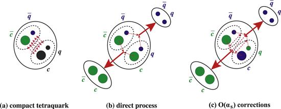
Figure 2. The decay of a compact tetraquark state into one charmonium meson and one light meson, which can happen through either (b) a direct fall-apart process, or (c) a process with gluons exchanged.
Together with table 1, we extract the following decay channels:

1. The decay of $| {0}_{{qc}}{1}_{\bar{q}\bar{c}};{1}^{++}\rangle $ into χc0η is contributed by ${I}^{S}\times {P}_{\mu }^{A}$:

$\begin{eqnarray}\begin{array}{l}\langle X(p,\epsilon )| {\chi }_{c0}({p}_{1})\,\eta ({p}_{2})\rangle \\ \approx -\displaystyle \frac{{\rm{i}}{c}_{1}}{3}\,{m}_{{\chi }_{c0}}{f}_{{\chi }_{c0}}{f}_{\eta }\,\epsilon \cdot {p}_{2}\equiv {g}_{{\chi }_{c0}\eta }\,\epsilon \cdot {p}_{2},\end{array}\end{eqnarray}$
where c1 is an overall factor, related to the coupling of ${\eta }_{\mu }^{{ \mathcal X }}(x,y)$ to the X(3872) as well as the dynamical process $(x,y)\Longrightarrow ({x}^{{\prime} },{y}^{{\prime} })$ shown in figure 2. This decay is kinematically forbidden.

2. According to ${I}^{S}\times {P}_{\mu }^{A}$, $| {0}_{{qc}}{1}_{\bar{q}\bar{c}};{1}^{++}\rangle $ can also decay into χc0f1(1285):

$\begin{eqnarray}| {0}_{{qc}}{1}_{\bar{q}\bar{c}};{1}^{++}\rangle \to {\chi }_{c0}{f}_{1}.\end{eqnarray}$
This decay is kinematically forbidden.

3. Decays of $| {0}_{{qc}}{1}_{\bar{q}\bar{c}};{1}^{++}\rangle $ into ηcf0(500) and χc1f0(500) are both contributed by ${I}_{\mu }^{A}\times {P}^{S}$:

$\begin{eqnarray}\begin{array}{l}\langle X(p,\epsilon )| {\eta }_{c}({p}_{1})\,{f}_{0}({p}_{2})\rangle \\ \approx \,+\,\displaystyle \frac{{\rm{i}}{c}_{1}}{3}\,{m}_{{f}_{0}}{f}_{{f}_{0}}{f}_{{\eta }_{c}}\,\epsilon \cdot {p}_{1}\equiv {g}_{{\eta }_{c}{f}_{0}}\,\epsilon \cdot {p}_{1},\end{array}\end{eqnarray}$
$\begin{eqnarray}\begin{array}{l}\langle X(p,\epsilon )| {\chi }_{c1}({p}_{1},{\epsilon }_{1})\,{f}_{0}({p}_{2})\rangle \\ \approx \,+\,\displaystyle \frac{{c}_{1}}{3}\,{m}_{{f}_{0}}{f}_{{f}_{0}}{m}_{{\chi }_{c1}}{f}_{{\chi }_{c1}}\,\epsilon \cdot {\epsilon }_{1}\equiv {g}_{{\chi }_{c1}{f}_{0}}\,\epsilon \cdot {\epsilon }_{1}.\end{array}\end{eqnarray}$
Because it is difficult to observe the f0(500) in experiments, in the present study we shall calculate widths of the $| {0}_{{qc}}{1}_{\bar{q}\bar{c}};{1}^{++}\rangle \to {\eta }_{c}{f}_{0}\to {\eta }_{c}\pi \pi $ and $| {0}_{{qc}}{1}_{\bar{q}\bar{c}};{1}^{++}\rangle \to {\chi }_{c1}{f}_{0}\to {\chi }_{c1}\pi \pi $ processes.

4. The decay of $| {0}_{{qc}}{1}_{\bar{q}\bar{c}};{1}^{++}\rangle $ into J/ψω is contributed by both IV,ν × PT,ρσ and IT,ρσ × PV,ν:

$\begin{eqnarray}\begin{array}{l}\langle X(p,\epsilon )| J/\psi ({p}_{1},{\epsilon }_{1})\,\omega ({p}_{2},{\epsilon }_{2})\rangle \\ \approx -\displaystyle \frac{{\rm{i}}{c}_{1}}{3}\,{\epsilon }_{\mu \nu \rho \sigma }{\epsilon }^{\mu }{\epsilon }_{1}^{\nu }{\epsilon }_{2}^{\rho }{p}_{2}^{\sigma }\,{m}_{J/\psi }{f}_{J/\psi }{f}_{\omega }^{T}\\ -\displaystyle \frac{{\rm{i}}{c}_{1}}{3}\,{\epsilon }_{\mu \nu \rho \sigma }{\epsilon }^{\mu }{\epsilon }_{1}^{\nu }{\epsilon }_{2}^{\rho }{p}_{1}^{\sigma }\,{m}_{\omega }{f}_{\omega }{f}_{J/\psi }^{T}\\ \equiv \,{g}_{\psi \omega }^{A}\,{\epsilon }_{\mu \nu \rho \sigma }{\epsilon }^{\mu }{\epsilon }_{1}^{\nu }{\epsilon }_{2}^{\rho }{p}_{2}^{\sigma }+{g}_{\psi \omega }^{B}\,{\epsilon }_{\mu \nu \rho \sigma }{\epsilon }^{\mu }{\epsilon }_{1}^{\nu }{\epsilon }_{2}^{\rho }{p}_{1}^{\sigma }.\end{array}\end{eqnarray}$
This decay is kinematically forbidden, but the $| {0}_{{qc}}{1}_{\bar{q}\bar{c}};{1}^{++}\rangle \to J/\psi \omega \to J/\psi \pi \pi \pi $ process is kinematically allowed.

5. According to IV,ν × PT,ρσ, $| {0}_{{qc}}{1}_{\bar{q}\bar{c}};{1}^{++}\rangle $ can also decay into J/ψh1(1170):

$\begin{eqnarray}\begin{array}{l}\langle X(p,\epsilon )| J/\psi ({p}_{1},{\epsilon }_{1})\,{h}_{1}({p}_{2},{\epsilon }_{2})\rangle \\ \approx \,+\,\displaystyle \frac{{\rm{i}}{c}_{1}}{6}\,{\epsilon }_{\mu \nu \rho \sigma }{\epsilon }_{\rho \sigma \alpha \beta }{\epsilon }^{\mu }{\epsilon }_{1}^{\nu }{\epsilon }_{2}^{\alpha }{p}_{2}^{\beta }\,{m}_{J/\psi }{f}_{J/\psi }{f}_{{h}_{1}}^{T}\\ \equiv \,{g}_{\psi {h}_{1}}\,{\epsilon }_{\mu \nu \rho \sigma }{\epsilon }_{\rho \sigma \alpha \beta }{\epsilon }^{\mu }{\epsilon }_{1}^{\nu }{\epsilon }_{2}^{\alpha }{p}_{2}^{\beta }.\end{array}\end{eqnarray}$
This decay is kinematically forbidden, but the $| {0}_{{qc}}{1}_{\bar{q}\bar{c}};{1}^{++}\rangle \to J/\psi {h}_{1}\to J/\psi \rho \pi \to J/\psi \pi \pi \pi $ process is kinematically allowed.

6. According to IT,ρσ × PV,ν, $| {0}_{{qc}}{1}_{\bar{q}\bar{c}};{1}^{++}\rangle $ can also decay into hcω:

$\begin{eqnarray}| {0}_{{qc}}{1}_{\bar{q}\bar{c}};{1}^{++}\rangle \to {h}_{c}\omega .\end{eqnarray}$
This decay is kinematically forbidden.

Summarizing the above results, we obtain numerically
$\begin{eqnarray}\begin{array}{l}{g}_{{\eta }_{c}{f}_{0}}\sim +{\rm{i}}{c}_{1}\,2.51\times {10}^{7}\,{\mathrm{MeV}}^{3},\\ {g}_{{\chi }_{c1}{f}_{0}}\sim +{c}_{1}\,0.76\times {10}^{11}\,{\mathrm{MeV}}^{4},\\ {g}_{\psi \omega }^{A}=-{\rm{i}}{c}_{1}\,6.86\times {10}^{7}\,{\mathrm{MeV}}^{3},\\ {g}_{\psi \omega }^{B}=-{\rm{i}}{c}_{1}\,2.31\times {10}^{7}\,{\mathrm{MeV}}^{3},\\ {g}_{\psi {h}_{1}}=+{\rm{i}}{c}_{1}\,3.88\times {10}^{7}\,{\mathrm{MeV}}^{3},\end{array}\end{eqnarray}$
from which we further obtain
$\begin{eqnarray}\begin{array}{l}\displaystyle \frac{{ \mathcal B }(| {0}_{{qc}}{1}_{\bar{q}\bar{c}};{1}^{++}\rangle \to {\eta }_{c}{f}_{0}\to {\eta }_{c}\pi \pi )}{{ \mathcal B }(| {0}_{{qc}}{1}_{\bar{q}\bar{c}};{1}^{++}\rangle \to J/\psi \omega \to J/\psi \pi \pi \pi )}\sim 0.091,\\ \displaystyle \frac{{ \mathcal B }(| {0}_{{qc}}{1}_{\bar{q}\bar{c}};{1}^{++}\rangle \to {\chi }_{c1}{f}_{0}\to {\chi }_{c1}\pi \pi )}{{ \mathcal B }(| {0}_{{qc}}{1}_{\bar{q}\bar{c}};{1}^{++}\rangle \to J/\psi \omega \to J/\psi \pi \pi \pi )}\sim 0.086,\\ \displaystyle \frac{{ \mathcal B }(| {0}_{{qc}}{1}_{\bar{q}\bar{c}};{1}^{++}\rangle \to J/\psi {h}_{1}\to J/\psi \pi \pi \pi )}{{ \mathcal B }(| {0}_{{qc}}{1}_{\bar{q}\bar{c}};{1}^{++}\rangle \to J/\psi \omega \to J/\psi \pi \pi \pi )}=1.4\times {10}^{-3}.\end{array}\end{eqnarray}$
Detailed calculations can be found in appendix A.

3.2. ${\eta }_{\mu }^{{ \mathcal X }}([{qc}][\bar{q}\bar{c}]) \rightarrow {\xi }_{\mu }^{i}([\bar{c}q]\,+\,[\bar{q}c])$

As depicted in figure 3, when the c and $\bar{q}$ quarks meet each other and the q and $\bar{c}$ quarks meet each other at the same time, a compact tetraquark state decays into two charmed mesons. This process can be described by the transformation (11):
$\begin{eqnarray}\begin{array}{l}{\eta }_{\mu }^{{ \mathcal X }}(x,y;I=0)\\ \Longrightarrow -\displaystyle \frac{1}{3}\,{\xi }_{\mu }^{1}({x}^{{\prime} },{y}^{{\prime} };I=0)+\displaystyle \frac{{\rm{i}}}{3}\,{\xi }_{\mu }^{4}({x}^{{\prime} },{y}^{{\prime} };I=0)\,+\,\cdots \\ =\,+\,\displaystyle \frac{{\rm{i}}}{3}\,{O}_{\mu }^{V}({x}^{{\prime} })\,{O}^{P}({y}^{{\prime} })+\displaystyle \frac{{\rm{i}}}{3}\,{O}^{A,\nu }({x}^{{\prime} })\,{O}_{\mu \nu }^{T}({y}^{{\prime} })\\ +\,{\rm{c}}.{\rm{c}}.\,+\,\cdots .\end{array}\end{eqnarray}$
Again, we keep only the direct fall-apart process described by ${\xi }_{\mu }^{1,4}$, but neglect the ${ \mathcal O }({\alpha }_{s})$ corrections described by ${\xi }_{\mu }^{5,8}$.
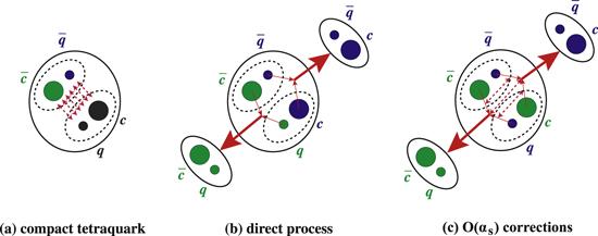
Figure 3. The decay of a compact tetraquark state into two charmed mesons, which can happen through either (b) a direct fall-apart process, or (c) a process with gluons exchanged.
The decay of $| {0}_{{qc}}{1}_{\bar{q}\bar{c}};{1}^{++}\rangle $ into the $D{\bar{D}}^{* }$ final state is contributed by both ${O}_{\mu }^{V}\times {O}^{P}$ and ${O}^{A,\nu }\times {O}_{\mu \nu }^{T}$:
$\begin{eqnarray}\begin{array}{l}\langle X(p,\epsilon )| {D}^{0}({p}_{1}){\bar{D}}^{* 0}({p}_{2},{\epsilon }_{2})\rangle \\ \approx \,+\,\displaystyle \frac{{\rm{i}}{c}_{2}}{3\sqrt{2}}\,{\lambda }_{D}{m}_{{D}^{* }}{f}_{{D}^{* }}\,\epsilon \cdot {\epsilon }_{2}\\ -\displaystyle \frac{{\rm{i}}{c}_{2}}{3\sqrt{2}}\,{f}_{D}{f}_{{D}^{* }}^{T}\,(\epsilon \cdot {p}_{2}\,{\epsilon }_{2}\cdot {p}_{1}-{p}_{1}\cdot {p}_{2}\,\epsilon \cdot {\epsilon }_{2})\\ \equiv \,{g}_{D{\bar{D}}^{* }}^{S}\,\epsilon \cdot {\epsilon }_{2}+{g}_{D{\bar{D}}^{* }}^{D}\,(\epsilon \cdot {p}_{2}\,{\epsilon }_{2}\cdot {p}_{1}-{p}_{1}\cdot {p}_{2}\,\epsilon \cdot {\epsilon }_{2}),\end{array}\end{eqnarray}$
where c2 is an overall factor, related to the coupling of ${\eta }_{\mu }^{{ \mathcal X }}(x,y)$ to the X(3872) as well as the dynamical process $(x,y)\Longrightarrow ({x}^{{\prime} },{y}^{{\prime} })$ shown in figure 3. This decay might be kinematically forbidden, but the $| {0}_{{qc}}{1}_{\bar{q}\bar{c}};{1}^{++}\rangle \to {D}^{0}{\bar{D}}^{* 0}+{D}^{* 0}{\bar{D}}^{0}\to {D}^{0}{\bar{D}}^{0}{\pi }^{0}$ process is surely kinematically allowed. The two coupling constants ${g}_{D{\bar{D}}^{* }}^{S}$ and ${g}_{D{\bar{D}}^{* }}^{D}$ are defined for the S- and D-wave $X(3872)\to D{\bar{D}}^{* }$ decays:
$\begin{eqnarray}{{ \mathcal L }}_{D{\bar{D}}^{* }}^{S}={g}_{D{\bar{D}}^{* }}^{S}\,{X}^{\mu }\,{D}^{0}\,{\bar{D}}_{\mu }^{* 0}\,+\,\cdots ,\end{eqnarray}$
$\begin{eqnarray}\begin{array}{l}{{ \mathcal L }}_{D{\bar{D}}^{* }}^{D}={g}_{D{\bar{D}}^{* }}^{D}\times \left({g}^{\mu \sigma }{g}^{\nu \rho }-{g}^{\mu \nu }{g}^{\rho \sigma }\right)\\ \times {X}^{\mu }\,{\partial }_{\rho }{D}^{0}\,{\partial }_{\sigma }{\bar{D}}_{\nu }^{* 0}+\cdots .\end{array}\end{eqnarray}$
Numerically, we obtain
$\begin{eqnarray}\begin{array}{rcl}{g}_{D{\bar{D}}^{* }}^{S} & = & +{\rm{i}}{c}_{2}\,0.69\times {10}^{11}\,{\mathrm{MeV}}^{4},\\ {g}_{D{\bar{D}}^{* }}^{D} & = & -{\rm{i}}{c}_{2}\,1.10\times {10}^{4}\,{\mathrm{MeV}}^{2}.\end{array}\end{eqnarray}$
Comparing this decay with the $| {0}_{{qc}}{1}_{\bar{q}\bar{c}};{1}^{++}\rangle \to J/\psi \omega \to J/\psi \pi \pi \pi $ decay studied in the previous subsection, we further obtain
$\begin{eqnarray}\begin{array}{l}\displaystyle \frac{{ \mathcal B }(| {0}_{{qc}}{1}_{\bar{q}\bar{c}};{1}^{++}\rangle \to {D}^{0}{\bar{D}}^{* 0}+{D}^{* 0}{\bar{D}}^{0}\to {D}^{0}{\bar{D}}^{0}{\pi }^{0})}{{ \mathcal B }(| {0}_{{qc}}{1}_{\bar{q}\bar{c}};{1}^{++}\rangle \to J/\psi \omega \to J/\psi \pi \pi \pi )}\\ =\,0.32\times \displaystyle \frac{{c}_{2}^{2}}{{c}_{1}^{2}}.\end{array}\end{eqnarray}$
Detailed calculations can also be found in appendix A. As proposed in [61], when the X(3872) decays, a constituent of the diquark must tunnel through the barrier of the diquark-antidiquark potential. However, this tunnelling for heavy quarks is exponentially suppressed compared to that for light quarks, so the compact tetraquark couplings are expected to favour the open charm modes with respect to charmonium ones. Accordingly, c2 may be significantly larger than c1, so that $| {0}_{{qc}}{1}_{\bar{q}\bar{c}};{1}^{++}\rangle $ may mainly decay into the ${D}^{0}{\bar{D}}^{0}{\pi }^{0}$ final state.

3.3. ${\eta }_{\mu }^{{ \mathcal X }}([{qc}][\bar{q}\bar{c}]) \rightarrow {\theta }_{\mu }^{1,2,3,4}([\bar{c}c]\,+\,[\bar{q}q])+{\xi }_{\mu }^{1,2,3,4}([\bar{c}q]\,+\,[\bar{q}c])$

If the above two processes investigated in section 3.1 and section 3.2 happen at the same time, i.e., $| {0}_{{qc}}{1}_{\bar{q}\bar{c}};{1}^{++}\rangle $ decays into one charmonium meson and one light meson as well as two charmed mesons simultaneously, we can use the transformation (12), which contains the color-singlet-color-singlet currents ${\theta }_{\mu }^{1,2,3,4}$ and ${\xi }_{\mu }^{1,2,3,4}$ together:
$\begin{eqnarray}\begin{array}{l}{\eta }_{\mu }^{{ \mathcal X }}(x,y;I=0)\\ \Longrightarrow -\displaystyle \frac{1}{2}\,{\theta }_{\mu }^{1}({x}^{{\prime} },{y}^{{\prime} };I=0)+\displaystyle \frac{1}{2}\,{\theta }_{\mu }^{2}({x}^{{\prime} },{y}^{{\prime} };I=0)\\ -\displaystyle \frac{{\rm{i}}}{2}\,{\theta }_{\mu }^{3}({x}^{{\prime} },{y}^{{\prime} };I=0)+\displaystyle \frac{{\rm{i}}}{2}\,{\theta }_{\mu }^{4}({x}^{{\prime} },{y}^{{\prime} };I=0)\\ -\displaystyle \frac{1}{2}\,{\xi }_{\mu }^{1}({x}^{{\prime\prime} },{y}^{{\prime\prime} };I=0)+\displaystyle \frac{{\rm{i}}}{2}\,{\xi }_{\mu }^{4}({x}^{{\prime\prime} },{y}^{{\prime\prime} };I=0).\end{array}\end{eqnarray}$
In the above expression we keep all terms, and there is no ⋯any more. Comparing this equation with equations (19) and (30), we obtain the same relative branching ratios as section 3.1 and section 3.2, just with the overall factors c1 and c2 replaced by others.

4. Decay properties of the X(3872) as a hadronic molecular state

Another possible interpretation of the X(3872) is the $D{\bar{D}}^{* }$ hadronic molecular state of JPC = 1++ [1824], i.e., $| D{\bar{D}}^{* };{1}^{++}\rangle $ defined in equation (6). Its relevant isoscalar current ${\xi }_{\mu }^{{ \mathcal X }}(x,y;I=0)$ is given in equation (7). We can transform it to ${\theta }_{\mu }^{i}(x,y;I=0)$ according to equation (13), through which we study decay properties of the X(3872) as an isoscalar hadronic molecular state in the following subsections.

4.1. ${\xi }_{\mu }^{{ \mathcal X }}([\bar{c}q][\bar{q}c])\to {\theta }_{\mu }^{i}([\bar{c}c]\,+\,[\bar{q}q])$

As depicted in figure 4, when the q and $\bar{q}$ quarks meet each other and the c and $\bar{c}$ quarks meet each other at the same time, a hadronic molecular state decays into one charmonium meson and one light meson. This process can be described by the transformation (13):
$\begin{eqnarray}\begin{array}{l}{\xi }_{\mu }^{{ \mathcal X }}(x,y;I=0)\\ \Longrightarrow +\displaystyle \frac{1}{6}\,{\theta }_{\mu }^{1}({x}^{{\prime} },{y}^{{\prime} };I=0)-\displaystyle \frac{1}{6}\,{\theta }_{\mu }^{2}({x}^{{\prime} },{y}^{{\prime} };I=0)\\ -\displaystyle \frac{{\rm{i}}}{6}\,{\theta }_{\mu }^{3}({x}^{{\prime} },{y}^{{\prime} };I=0)+\displaystyle \frac{{\rm{i}}}{6}\,{\theta }_{\mu }^{4}({x}^{{\prime} },{y}^{{\prime} };I=0)\,+\,\cdots \\ =+\displaystyle \frac{1}{6}\,{I}^{S}({x}^{{\prime} })\,{P}_{\mu }^{A}({y}^{{\prime} })-\displaystyle \frac{1}{6}\,{I}_{\mu }^{A}({x}^{{\prime} })\,{P}^{S}({y}^{{\prime} })\\ +\displaystyle \frac{1}{12}\,{\epsilon }_{\mu \nu \rho \sigma }\,{I}^{V,\nu }({x}^{{\prime} })\,{P}^{T,\rho \sigma }({y}^{{\prime} })\\ -\displaystyle \frac{1}{12}\,{\epsilon }_{\mu \nu \rho \sigma }\,{I}^{T,\rho \sigma }({x}^{{\prime} })\,{P}^{V,\nu }({y}^{{\prime} })\,+\,\cdots .\end{array}\end{eqnarray}$
Here we keep only the direct fall-apart process described by ${\theta }_{\mu }^{1,2,3,4}$, but neglect the ${ \mathcal O }({\alpha }_{s})$ corrections described by ${\theta }_{\mu }^{5,6,7,8}$.
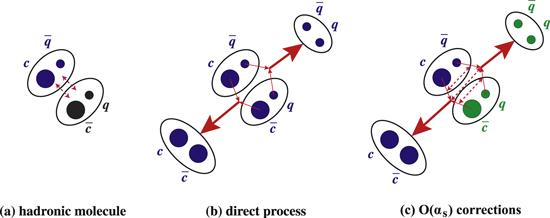
Figure 4. The decay of a hadronic molecular state into one charmonium meson and one light meson, which can happen through either (b) a direct fall-apart process, or (c) a process with gluons exchanged.
We repeat the same procedures as those done in section 3.1, and extract the following coupling constants from this transformation:
$\begin{eqnarray}\begin{array}{rcl}{h}_{{\eta }_{c}{f}_{0}} & \sim & -{\rm{i}}{c}_{1}\,1.26\times {10}^{7}\,{\mathrm{MeV}}^{3},\\ {h}_{{\chi }_{c1}{f}_{0}} & \sim & -{c}_{1}\,0.38\times {10}^{11}\,{\mathrm{MeV}}^{4},\\ {h}_{\psi \omega }^{A} & = & -{\rm{i}}{c}_{4}\,3.43\times {10}^{7}\,{\mathrm{MeV}}^{3},\\ {h}_{\psi \omega }^{B} & = & -{\rm{i}}{c}_{4}\,1.16\times {10}^{7}\,{\mathrm{MeV}}^{3},\\ {h}_{\psi {h}_{1}} & = & +{\rm{i}}{c}_{4}\,1.94\times {10}^{7}\,{\mathrm{MeV}}^{3}.\end{array}\end{eqnarray}$
They are defined for the $| D{\bar{D}}^{* };{1}^{++}\rangle \to {\eta }_{c}{f}_{0}$, χc1f0, J/ψω, and J/ψh1 decays. They all contain an overall factor c4, which is related to the coupling of ${\xi }_{\mu }^{{ \mathcal X }}(x,y)$ to the X(3872) as well as the dynamical process $(x,y)\Longrightarrow ({x}^{{\prime} },{y}^{{\prime} })$ shown in figure 4.
Using these coupling constants, we further obtain
$\begin{eqnarray}\begin{array}{l}\displaystyle \frac{{ \mathcal B }(| D{\bar{D}}^{* };{1}^{++}\rangle \to {\eta }_{c}{f}_{0}\to {\eta }_{c}\pi \pi )}{{ \mathcal B }(| D{\bar{D}}^{* };{1}^{++}\rangle \to J/\psi \omega \to J/\psi \pi \pi \pi )}\sim 0.091,\\ \displaystyle \frac{{ \mathcal B }(| D{\bar{D}}^{* };{1}^{++}\rangle \to {\chi }_{c1}{f}_{0}\to {\chi }_{c1}\pi \pi )}{{ \mathcal B }(| D{\bar{D}}^{* };{1}^{++}\rangle \to J/\psi \omega \to J/\psi \pi \pi \pi )}\sim 0.086,\\ \displaystyle \frac{{ \mathcal B }(| D{\bar{D}}^{* };{1}^{++}\rangle \to J/\psi {h}_{1}\to J/\psi \pi \pi \pi )}{{ \mathcal B }(| D{\bar{D}}^{* };{1}^{++}\rangle \to J/\psi \omega \to J/\psi \pi \pi \pi )}=1.4\times {10}^{-3},\end{array}\end{eqnarray}$
which ratios are the same as equations (29), obtained in section 3.1 for the compact tetraquark state $| {0}_{{qc}}{1}_{\bar{q}\bar{c}};{1}^{++}\rangle $.

4.2. ${\xi }_{\mu }^{{ \mathcal X }}([\bar{c}q][\bar{q}c])\to {\xi }_{\mu }^{i}([\bar{c}q]\,+\,[\bar{q}c])$

Assuming the X(3872) to be the $D{\bar{D}}^{* }$ hadronic molecular state of JPC = 1++, it can naturally decay into the $D{\bar{D}}^{* }$ final state, which fall-apart process can be described by itself:
$\begin{eqnarray}\begin{array}{l}{\xi }_{\mu }^{{ \mathcal Z }}(x,y;I=0)\Longrightarrow {\xi }_{\mu }^{1}({x}^{{\prime} },{y}^{{\prime} };I=0)\\ =-{\rm{i}}\,{O}_{\mu }^{V}({x}^{{\prime} })\,{O}^{P}({y}^{{\prime} })+{\rm{c}}.{\rm{c}}.,\end{array}\end{eqnarray}$
and so
$\begin{eqnarray}\begin{array}{l}\langle X(p,\epsilon )| {D}^{0}({p}_{1}){\bar{D}}^{* 0}({p}_{2},{\epsilon }_{2})\rangle \approx -\displaystyle \frac{{\rm{i}}{c}_{5}}{\sqrt{2}}\,{\lambda }_{D}{m}_{{D}^{* }}{f}_{{D}^{* }}\,\epsilon \cdot {\epsilon }_{2}\\ \equiv \,{h}_{D{\bar{D}}^{* }}\,\epsilon \cdot {\epsilon }_{2},\end{array}\end{eqnarray}$
where c5 is an overall factor. Again, this decay might be kinematically forbidden, but the $| D{\bar{D}}^{* };{1}^{++}\rangle \to {D}^{0}{\bar{D}}^{* 0}\,+{D}^{* 0}{\bar{D}}^{0}\to {D}^{0}{\bar{D}}^{0}{\pi }^{0}$ process is surely kinematically allowed.
Numerically, we obtain
$\begin{eqnarray}\begin{array}{rcl}{h}_{D{\bar{D}}^{* }}^{S} & = & -{\rm{i}}{c}_{5}\,2.1\times {10}^{11}\,{\mathrm{MeV}}^{4},\\ {h}_{D{\bar{D}}^{* }}^{D} & = & 0.\end{array}\end{eqnarray}$
Comparing this decay with the $| D{\bar{D}}^{* };{1}^{++}\rangle \to J/\psi \omega \to J/\psi \pi \pi \pi $ decay studied in the previous subsection, we further obtain
$\begin{eqnarray}\begin{array}{l}\displaystyle \frac{{ \mathcal B }(| D{\bar{D}}^{* };{1}^{++}\rangle \to {D}^{0}{\bar{D}}^{* 0}+{D}^{* 0}{\bar{D}}^{0}\to {D}^{0}{\bar{D}}^{0}{\pi }^{0})}{{ \mathcal B }(| D{\bar{D}}^{* };{1}^{++}\rangle \to J/\psi \omega \to J/\psi \pi \pi \pi )}\\ \quad =\,4.5\times \displaystyle \frac{{c}_{5}^{2}}{{c}_{4}^{2}}.\end{array}\end{eqnarray}$
Therefore, $| D{\bar{D}}^{* };{1}^{++}\rangle $ mainly decays into two charmed mesons, because c5 is probably larger than c4.

5. Isospin of the X(3872)

The isospin breaking effect of the X(3872) is significant and important to understand its nature [310]. As proposed in [78], this can be simply because the close proximity of the mass of the isoscalar X(3872) to the neutral ${D}^{0}{\bar{D}}^{* 0}$ threshold. We argue that in this case the X(3872) and the ${D}^{0}{\bar{D}}^{* 0}$ threshold together can be considered as a ‘mixed’ state, not purely isoscalar any more, through which we can investigate the isovector decay channels of the X(3872).
In this section we shall investigate the isospin breaking effect of the X(3872) by freely choosing its quark content [12, 65, 66], for example,
$\begin{eqnarray}\begin{array}{l}{\eta }_{\mu }^{1}(\theta /{\theta }^{{\prime} })=\cos \theta \,{\eta }_{\mu }^{1}([{uc}][\bar{u}\bar{c}])+\sin \theta \,{\eta }_{\mu }^{1}([{dc}][\bar{d}\bar{c}])\\ =\,\cos \theta \times \left({u}_{a}^{{\rm{T}}}{\mathbb{C}}{\gamma }_{\mu }{c}_{b}\,{\bar{u}}_{a}{\gamma }_{5}{\mathbb{C}}{\bar{c}}_{b}^{{\rm{T}}}+\{{\gamma }_{\mu }\leftrightarrow {\gamma }_{5}\}\right)\\ +\,\sin \theta \times \{u/\bar{u}\to d/\bar{d}\}\\ \Rightarrow \,\cos {\theta }^{{\prime} }\,{\eta }_{\mu }^{1}(I=0)+\sin {\theta }^{{\prime} }\,{\eta }_{\mu }^{1}(I=1),\end{array}\end{eqnarray}$
where θ and ${\theta }^{{\prime} }$ are the two related mixing angles. We shall fine-tune them to be different from $\theta =45^\circ /{\theta }^{{\prime} }=0^\circ $, so that the X(3872) is assumed not to be a purely isoscalar state. We shall study this effect separately for the compact tetraquark and hadronic molecule scenarios in the following subsections.

5.1. Isospin breaking effect of $| {0}_{{qc}}{1}_{\bar{q}\bar{c}};{1}^{++}\rangle $

We repeat the same procedures as those done in section 3.1, and transform ${\eta }_{\mu }^{{ \mathcal X }}(x,y;{\theta }_{1}^{{\prime} })$ to ${\theta }_{\mu }^{i}(x,y;{\theta }_{1}^{{\prime} })$ according to equation (10), from which we extract the following isovector decay channels:

1. The decay of $| {0}_{{qc}}{1}_{\bar{q}\bar{c}};{1}^{++}\rangle $ into χc0π is contributed by ${I}^{S}\times {J}_{\mu }^{A}$:

$\begin{eqnarray}\begin{array}{l}\langle X(p,\epsilon )| {\chi }_{c0}({p}_{1})\,\pi ({p}_{2})\rangle \\ \approx -\displaystyle \frac{{\rm{i}}{c}_{1}\sin {\theta }_{1}^{{\prime} }}{3}\,{m}_{{\chi }_{c0}}{f}_{{\chi }_{c0}}{f}_{\pi }\,\epsilon \cdot {p}_{2}\equiv {g}_{{\chi }_{c0}\pi }\,\epsilon \cdot {p}_{2}.\end{array}\end{eqnarray}$
This process is kinematically allowed.

2. The decay of $| {0}_{{qc}}{1}_{\bar{q}\bar{c}};{1}^{++}\rangle $ into J/ψρ is contributed by both IV,ν × JT,ρσ and IT,ρσ × JV,ν:

$\begin{array}{l}\langle X(p,\epsilon )| J/\psi ({p}_{1},{\epsilon }_{1})\,\rho ({p}_{2},{\epsilon }_{2})\rangle \\ \approx -\displaystyle \frac{{\rm{i}}{c}_{1}\sin {\theta }_{1}^{{\prime} }}{3}\,{\epsilon }_{\mu \nu \rho \sigma }{\epsilon }^{\mu }{\epsilon }_{1}^{\nu }{\epsilon }_{2}^{\rho }{p}_{2}^{\sigma }\,{m}_{J/\psi }{f}_{J/\psi }{f}_{\rho }^{T}\\ -\displaystyle \frac{{\rm{i}}{c}_{1}\sin {\theta }_{1}^{{\prime} }}{3}\,{\epsilon }_{\mu \nu \rho \sigma }{\epsilon }^{\mu }{\epsilon }_{1}^{\nu }{\epsilon }_{2}^{\rho }{p}_{1}^{\sigma }\,{m}_{\rho }{f}_{\rho }{f}_{J/\psi }^{T}\\ \equiv \,{g}_{\psi \rho }^{A}\,{\epsilon }_{\mu \nu \rho \sigma }{\epsilon }^{\mu }{\epsilon }_{1}^{\nu }{\epsilon }_{2}^{\rho }{p}_{2}^{\sigma }+{g}_{\psi \rho }^{B}\,{\epsilon }_{\mu \nu \rho \sigma }{\epsilon }^{\mu }{\epsilon }_{1}^{\nu }{\epsilon }_{2}^{\rho }{p}_{1}^{\sigma }.\end{array}$
If we use ${m}_{{\rho }^{0}}=775.26\,\mathrm{MeV}$ [2], this decay would be kinematically forbidden, but the $| {0}_{{qc}}{1}_{\bar{q}\bar{c}};{1}^{++}\rangle \,\to J/\psi \rho \to J/\psi \pi \pi $ process is surely kinematically allowed.

Numerically, we obtain
$\begin{eqnarray}\begin{array}{rcl}{g}_{{\chi }_{c0}\pi } & = & -{\rm{i}}{c}_{1}\sin {\theta }_{1}^{{\prime} }\,5.08\times {10}^{7}\,{\mathrm{MeV}}^{3},\\ {g}_{\psi \rho }^{A} & = & -{\rm{i}}{c}_{1}\sin {\theta }_{1}^{{\prime} }\,6.86\times {10}^{7}\,{\mathrm{MeV}}^{3},\\ {g}_{\psi \rho }^{B} & = & -{\rm{i}}{c}_{1}\sin {\theta }_{1}^{{\prime} }\,2.29\times {10}^{7}\,{\mathrm{MeV}}^{3}.\end{array}\end{eqnarray}$
Comparing these decays with the $| {0}_{{qc}}{1}_{\bar{q}\bar{c}};{1}^{++}\rangle \to J/\psi \omega \to J/\psi \pi \pi \pi $ decay studied in section 3.1 (a factor ${\cos }^{2}{\theta }_{1}^{{\prime} }$ needs to be multiplied there), we can use ${\theta }_{1}^{{\prime} }=\pm 15^\circ $ to obtain
$\begin{eqnarray}\begin{array}{l}\displaystyle \frac{{ \mathcal B }(| {0}_{{qc}}{1}_{\bar{q}\bar{c}};{1}^{++}\rangle \to {\chi }_{c0}\pi )}{{ \mathcal B }(| {0}_{{qc}}{1}_{\bar{q}\bar{c}};{1}^{++}\rangle \to J/\psi \rho \to J/\psi \pi \pi )}=0.024,\\ \displaystyle \frac{{ \mathcal B }(| {0}_{{qc}}{1}_{\bar{q}\bar{c}};{1}^{++}\rangle \to J/\psi \omega \to J/\psi \pi \pi \pi )}{{ \mathcal B }(| {0}_{{qc}}{1}_{\bar{q}\bar{c}};{1}^{++}\rangle \to J/\psi \rho \to J/\psi \pi \pi )}=1.6,\end{array}\end{eqnarray}$
where the latter ratio has been fine-tuned to be the same as the recent BESIII experiment [41].
The isospin breaking effect can also affect the branching ratio of the $| {0}_{{qc}}{1}_{\bar{q}\bar{c}};{1}^{++}\rangle \to {D}^{0}{\bar{D}}^{* 0}+{D}^{* 0}{\bar{D}}^{0}\to {D}^{0}{\bar{D}}^{0}{\pi }^{0}$ decay. Using ${\theta }_{1}^{{\prime} }=+15^\circ $, we obtain
$\begin{eqnarray}\begin{array}{l}\displaystyle \frac{{ \mathcal B }(| {0}_{{qc}}{1}_{\bar{q}\bar{c}};{1}^{++}\rangle \to {D}^{0}{\bar{D}}^{* 0}+{D}^{* 0}{\bar{D}}^{0}\to {D}^{0}{\bar{D}}^{0}{\pi }^{0})}{{ \mathcal B }(| {0}_{{qc}}{1}_{\bar{q}\bar{c}};{1}^{++}\rangle \to J/\psi \omega \to J/\psi \pi \pi \pi )}\,=\,0.52\times \displaystyle \frac{{c}_{2}^{2}}{{c}_{1}^{2}},\end{array}\end{eqnarray}$
while using ${\theta }_{1}^{{\prime} }=-15^\circ $, this ratio is calculated to be around $0.17\times {c}_{2}^{2}/{c}_{1}^{2}$.

5.2. Isospin breaking effect of $| D{\bar{D}}^{* };{1}^{++}\rangle $

We repeat the same procedures as those done in section 4.1, and transform ${\xi }_{\mu }^{{ \mathcal X }}(x,y;{\theta }_{2}^{{\prime} })$ to ${\theta }_{\mu }^{i}(x,y;{\theta }_{2}^{{\prime} })$ according to equation (13), from which we extract the following isovector coupling constants:
$\begin{eqnarray}\begin{array}{rcl}{h}_{{\chi }_{c0}\pi } & = & +{\rm{i}}{c}_{4}\sin {\theta }_{2}^{{\prime} }\,2.54\times {10}^{7}\,{\mathrm{MeV}}^{3},\\ {h}_{\psi \rho }^{A} & = & -{\rm{i}}{c}_{4}\sin {\theta }_{2}^{{\prime} }\,3.43\times {10}^{7}\,{\mathrm{MeV}}^{3},\\ {h}_{\psi \rho }^{B} & = & -{\rm{i}}{c}_{4}\sin {\theta }_{2}^{{\prime} }\,1.14\times {10}^{7}\,{\mathrm{MeV}}^{3}.\end{array}\end{eqnarray}$
They are defined for the $| D{\bar{D}}^{* };{1}^{++}\rangle \to {\chi }_{c0}\pi $ and J/ψρ decays.
We can use the same angle ${\theta }_{2}^{{\prime} }=\pm 15^\circ $ to obtain
$\begin{eqnarray}\begin{array}{l}\displaystyle \frac{{ \mathcal B }(| D{\bar{D}}^{* };{1}^{++}\rangle \to {\chi }_{c0}\pi )}{{ \mathcal B }(| D{\bar{D}}^{* };{1}^{++}\rangle \to J/\psi \rho \to J/\psi \pi \pi )}=0.024,\\ \displaystyle \frac{{ \mathcal B }(| D{\bar{D}}^{* };{1}^{++}\rangle \to J/\psi \omega \to J/\psi \pi \pi \pi )}{{ \mathcal B }(| D{\bar{D}}^{* };{1}^{++}\rangle \to J/\psi \rho \to J/\psi \pi \pi )}=1.6,\end{array}\end{eqnarray}$
which ratios are the same as equations (48), obtained in the previous subsection for the compact tetraquark state $| {0}_{{qc}}{1}_{\bar{q}\bar{c}};{1}^{++}\rangle $.
Again, the isospin breaking effect can affect the branching ratio of the $| D{\bar{D}}^{* };{1}^{++}\rangle \to {D}^{0}{\bar{D}}^{* 0}+{D}^{* 0}{\bar{D}}^{0}\to {D}^{0}{\bar{D}}^{0}{\pi }^{0}$ decay. Using ${\theta }_{2}^{{\prime} }=+15^\circ $, we obtain
$\begin{eqnarray}\begin{array}{l}\displaystyle \frac{{ \mathcal B }(| D{\bar{D}}^{* };{1}^{++}\rangle \to {D}^{0}{\bar{D}}^{* 0}+{D}^{* 0}{\bar{D}}^{0}\to {D}^{0}{\bar{D}}^{0}{\pi }^{0})}{{ \mathcal B }(| D{\bar{D}}^{* };{1}^{++}\rangle \to J/\psi \omega \to J/\psi \pi \pi \pi )}\,=\,7.4\times \displaystyle \frac{{c}_{5}^{2}}{{c}_{4}^{2}},\end{array}\end{eqnarray}$
while using ${\theta }_{2}^{{\prime} }=-15^\circ $, this ratio is calculated to be around $2.4\times {c}_{5}^{2}/{c}_{4}^{2}$.

6. Summary and discussions

In this paper we systematically construct the tetraquark currents of JPC = 1++ with the quark content $c\bar{c}q\bar{q}$ (q=u/d). We consider three configurations, $[{cq}][\bar{c}\bar{q}]$, $[\bar{c}q][\bar{q}c]$, and $[\bar{c}c][\bar{q}q]$, and we construct eight independent currents for each of them. Their relations are derived using the Fierz rearrangement of the Dirac and color indices, through which we study decay properties of the X(3872):

Based on the transformation of $[{qc}][\bar{q}\bar{c}]\to [\bar{c}c][\bar{q}q]$, we study decay properties of the X(3872) as a compact tetraquark state into one charmonium meson and one light meson.

Based on the transformation of $[{qc}][\bar{q}\bar{c}]\to [\bar{c}q][\bar{q}c]$, we study decay properties of the X(3872) as a compact tetraquark state into two charmed mesons.

Based on the transformation of the $[{qc}][\bar{q}\bar{c}]$ currents to the color-singlet-color-singlet $[\bar{c}c][\bar{q}q]$ and $[\bar{c}q][\bar{q}c]$ currents, we obtain the same relative branching ratios as those obtained using the above two transformations.

Based on the transformation of $[\bar{c}q][\bar{q}c]\to [\bar{c}c][\bar{q}q]$, we study decay properties of the X(3872) as a hadronic molecular state into one charmonium meson and one light meson.

Based on the $[\bar{c}q][\bar{q}c]$ currents themselves, we study decay properties of the X(3872) as a hadronic molecular state into two charmed mesons.

We first use isoscalar tetraquark currents to study decay properties of the X(3872) as a purely isoscalar state, and then use isovector tetraquark currents to investigate its isospin breaking effect. The extracted relative branching ratios are summarized in table 2, where we have investigated the following interpretations of the X(3872):

In the second, third, and fourth columns of table 2, $| {0}_{{qc}}{1}_{\bar{q}\bar{c}};{1}^{++}\rangle $ denotes the compact tetraquark state of JPC = 1++, defined in equation (3). $| {0}_{{qc}}{1}_{\bar{q}\bar{c}};{1}^{++}\rangle $ with I = 0 (${\theta }_{1}^{{\prime} }=0^\circ $) is the purely isoscalar state, and those with ${\theta }_{1}^{{\prime} }=\pm 15^\circ $ contain some isovector components. Using the mixing angle ${\theta }_{1}^{{\prime} }=+{15}^{{\rm{o}}}$, we obtain

$\begin{eqnarray}\begin{array}{l}\displaystyle \frac{{ \mathcal B }\left(| {0}_{{qc}}{1}_{\bar{q}\bar{c}};{1}^{++}\rangle \to J/\psi \omega (\to \pi \pi \pi ):\,\,J/\psi \rho (\to \pi \pi )\,:\,\,{\chi }_{c0}\pi \,:{\eta }_{c}{f}_{0}(\to \pi \pi ):{\chi }_{c1}{f}_{0}(\to \pi \pi ):{D}^{0}{\bar{D}}^{* 0}(\to {D}^{0}{\bar{D}}^{0}{\pi }^{0})\,\right)}{{ \mathcal B }\left(| {0}_{{qc}}{1}_{\bar{q}\bar{c}};{1}^{++}\rangle \to J/\psi \omega (\to \pi \pi \pi )\right)}\\ \qquad \sim 1:0.63\,(\mathrm{input})\,\,:\,0.015\,:\,\,0.091\,(?):0.086(?):0.52\,{t}_{1}\,,\end{array}\end{eqnarray}$
while using the mixing angle ${\theta }_{1}^{{\prime} }=-{15}^{{\rm{o}}}$, we obtain
$\begin{eqnarray}\begin{array}{l}\displaystyle \frac{{ \mathcal B }\left(| {0}_{{qc}}{1}_{\bar{q}\bar{c}};{1}^{++}\rangle \to J/\psi \omega (\to \pi \pi \pi ):\,\,J/\psi \rho (\to \pi \pi )\,:\,\,{\chi }_{c0}\pi \,:{\eta }_{c}{f}_{0}(\to \pi \pi ):{\chi }_{c1}{f}_{0}(\to \pi \pi ):{D}^{0}{\bar{D}}^{* 0}(\to {D}^{0}{\bar{D}}^{0}{\pi }^{0})\,\right)}{{ \mathcal B }\left(| {0}_{{qc}}{1}_{\bar{q}\bar{c}};{1}^{++}\rangle \to J/\psi \omega (\to \pi \pi \pi )\right)}\\ \sim 1:\,\,0.63\,(\mathrm{input})\,\,:\,0.015\,:\,\,0.091\,(?)\,:\,\,\,0.086\,(?)\,\,:\,\,\,\,\,\,\,0.17\,{t}_{1}\,.\end{array}\end{eqnarray}$

In the fifth, sixth, and seventh columns of table 2, $| D{\bar{D}}^{* };{1}^{++}\rangle $ denotes the hadronic molecular state of JPC = 1++, defined in equation (6). $| D{\bar{D}}^{* };{1}^{++}\rangle $ with I = 0 (${\theta }_{2}^{{\prime} }=0^\circ $) is the purely isoscalar state, and those with ${\theta }_{2}^{{\prime} }=\pm 15^\circ $ contain some isovector components. Using the mixing angle ${\theta }_{2}^{{\prime} }=+{15}^{{\rm{o}}}$, we obtain

$\begin{eqnarray}\begin{array}{l}\displaystyle \frac{{ \mathcal B }\left(| D{\bar{D}}^{* };{1}^{++}\rangle \to J/\psi \omega (\to \pi \pi \pi ):\,\,J/\psi \rho (\to \pi \pi )\,:\,{\chi }_{c0}\pi \,:{\eta }_{c}{f}_{0}(\to \pi \pi ):{\chi }_{c1}{f}_{0}(\to \pi \pi ):{D}^{0}{\bar{D}}^{* 0}(\to {D}^{0}{\bar{D}}^{0}{\pi }^{0})\,\right)}{{ \mathcal B }\left(| D{\bar{D}}^{* };{1}^{++}\rangle \to J/\psi \omega (\to \pi \pi \pi )\right)}\\ \sim 1:\,\,0.63\,(\mathrm{input})\,\,:\,0.015\,:\,\,0.091\,(?)\,:\,\,\,0.086\,(?)\,\,:\,\,\,\,\,\,\,7.4\,{t}_{2}\,,\end{array}\end{eqnarray}$
while using the mixing angle ${\theta }_{2}^{{\prime} }=-{15}^{{\rm{o}}}$, we obtain
$\begin{eqnarray}\begin{array}{l}\displaystyle \frac{{ \mathcal B }\left(| D{\bar{D}}^{* };{1}^{++}\rangle \to J/\psi \omega (\to \pi \pi \pi ):\,\,J/\psi \rho (\to \pi \pi )\,:\,{\chi }_{c0}\pi \,:{\eta }_{c}{f}_{0}(\to \pi \pi ):{\chi }_{c1}{f}_{0}(\to \pi \pi ):{D}^{0}{\bar{D}}^{* 0}(\to {D}^{0}{\bar{D}}^{0}{\pi }^{0})\,\right)}{{ \mathcal B }\left(| D{\bar{D}}^{* };{1}^{++}\rangle \to J/\psi \omega (\to \pi \pi \pi )\right)}\\ \sim 1:\,\,0.63\,(\mathrm{input})\,\,:\,0.015\,:\,\,0.091\,(?)\,:\,\,\,0.086\,(?)\,\,:\,\,\,\,\,\,\,2.4\,{t}_{2}\,.\end{array}\end{eqnarray}$

Table 2. Relative branching ratios of the X(3872) evaluated through the Fierz rearrangement. ${\theta }_{1,2}^{{\prime} }$ are the two angles related to the isospin breaking effect, which are fine-tuned to be ${\theta }_{1}^{{\prime} }={\theta }_{2}^{{\prime} }=\pm {15}^{{\rm{o}}}$, so that $\displaystyle \frac{{ \mathcal B }(| {0}_{{qc}}{1}_{\bar{q}\bar{c}};{1}^{++}\rangle \to J/\psi \omega \to J/\psi \pi \pi \pi )}{{ \mathcal B }(| {0}_{{qc}}{1}_{\bar{q}\bar{c}};{1}^{++}\rangle \to J/\psi \rho \to J/\psi \pi \pi )}$ $=\displaystyle \frac{{ \mathcal B }(| D{\bar{D}}^{* };{1}^{++}\rangle \to J/\psi \omega \to J/\psi \pi \pi \pi )}{{ \mathcal B }(| D{\bar{D}}^{* };{1}^{++}\rangle \to J/\psi \rho \to J/\psi \pi \pi )}=1.6$ [41].
Channels $| {0}_{{qc}}{1}_{\bar{q}\bar{c}};{1}^{++}\rangle $ $| D{\bar{D}}^{* };{1}^{++}\rangle $
$I=0/{\theta }_{1}^{{\prime} }={0}^{{\rm{o}}}$ ${\theta }_{1}^{{\prime} }=+{15}^{{\rm{o}}}$ ${\theta }_{1}^{{\prime} }=-{15}^{{\rm{o}}}$ $I=0/{\theta }_{2}^{{\prime} }={0}^{{\rm{o}}}$ ${\theta }_{2}^{{\prime} }=+{15}^{{\rm{o}}}$ ${\theta }_{2}^{{\prime} }=-{15}^{{\rm{o}}}$
$\displaystyle \frac{{ \mathcal B }(X\to {\eta }_{c}{f}_{0}\to {\eta }_{c}\pi \pi )}{{ \mathcal B }(X\to J/\psi \omega \to J/\psi \pi \pi \pi )}$ ∼0.091 ∼0.091 ∼0.091 ∼0.091 ∼0.091 ∼0.091
$\displaystyle \frac{{ \mathcal B }(X\to {\chi }_{c1}{f}_{0}\to {\chi }_{c1}\pi \pi )}{{ \mathcal B }(X\to J/\psi \omega \to J/\psi \pi \pi \pi )}$ ∼0.086 ∼0.086 ∼0.086 ∼0.086 ∼0.086 ∼0.086
$\displaystyle \frac{{ \mathcal B }(X\to J/\psi {h}_{1}\to J/\psi \pi \pi \pi )}{{ \mathcal B }(X\to J/\psi \omega \to J/\psi \pi \pi \pi )}$ 1.4 × 10⁻³ 1.4 × 10⁻³ 1.4 × 10⁻³ 1.4 × 10⁻³ 1.4 × 10⁻³ 1.4 × 10⁻³
$\displaystyle \frac{{ \mathcal B }(X\to {\chi }_{c0}\pi )}{{ \mathcal B }(X\to J/\psi \rho \to J/\psi \pi \pi )}$ 0.024 0.024 0.024 0.024
$\displaystyle \frac{{ \mathcal B }(X\to J/\psi \omega \to J/\psi \pi \pi \pi )}{{ \mathcal B }(X\to J/\psi \rho \to J/\psi \pi \pi )}$ 1.6 (input) 1.6 (input) 1.6 (input) 1.6 (input)
$\displaystyle \frac{{ \mathcal B }(X\to {D}^{0}{\bar{D}}^{* 0}+{D}^{* 0}{\bar{D}}^{0}\to {D}^{0}{\bar{D}}^{0}{\pi }^{0})}{{ \mathcal B }(X\to J/\psi \omega \to J/\psi \pi \pi \pi )}$ 0.32 t1 0.52 t1 0.17 t1 4.5 t2 7.4 t2 2.4 t2
In the above expressions, we define the ratio ${t}_{1}\equiv {c}_{2}^{2}/{c}_{1}^{2}$ to be the parameter measuring which process happens more easily, the process depicted in figure 2(b) or the process depicted in figure 3(b). Because the exchange of one light quark with another light quark seems to be easier than the exchange of one light quark with another heavy quark [61, 79], it can be the case that t1 ≥ 1. As discussed in section 4.2, c5 is probably larger than c4, so that the other ratio ${t}_{2}\equiv {c}_{5}^{2}/{c}_{4}^{2}\geqslant 1$.
The above relative branching ratios extracted in the present study turn out to be very much different. This might be one of the reasons why many multiquark states were observed only in a few decay channels [49]. We note that in this paper we only consider the leading-order fall-apart decays described by color-singlet-color-singlet meson-meson currents, but neglect the ${ \mathcal O }({\alpha }_{s})$ corrections described by color-octet-color-octet meson-meson currents, so there can be other possible decay channels, such as X(3872) → χc1π [45]. Besides, there is still one parameter not considered in above analyses, that is the phase angle between S- and D-wave coupling constants. We shall investigate its relevant uncertainty in B.
Based on table 2, we conclude this paper. Generally speaking, compared to the Zc(3900) studied in [49], the results of this paper suggest that decay channels of the X(3872) are quite limited:

The X(3872) can couple to the χc0η, χc0f1(1285), and hcω channels, but all of them are kinematically forbidden.

The X(3872) can couple to the isovector channels J/ψρ and χc0π, but both of them are due to the isospin breaking effect.

The X(3872) can couple to the ${D}^{0}{\bar{D}}^{* 0}$ and J/ψρ channels, but its mass is very close to the relevant thresholds. Hence, in the present study we calculate widths of the three-body decays $X\to {D}^{0}{\bar{D}}^{* 0}+{D}^{* 0}{\bar{D}}^{0}\to {D}^{0}{\bar{D}}^{0}{\pi }^{0}$ and XJ/ψρJ/ψππ.

The X(3872) can couple to the J/ψω and J/ψh1(1170) channels, but both of them are kinematically forbidden. Hence, in the present study we calculate widths of the four-body decays XJ/ψωJ/ψπππ and XJ/ψh1J/ψπππ.

The decay processes Xηcf0ηcππ and Xχc1f0χc1ππ might be possible. In this paper we simply use the f0(500) to estimate widths of these two processes, but note that the obtained results do significantly depend on the nature of light scalar mesons, which are still quite ambiguous [77].

To end this paper, we give several comments and proposals:

The hadronic molecular state $| D{\bar{D}}^{* };{1}^{++}\rangle $ mainly decays into two charmed mesons, because c5 is probably larger than c4. The compact tetraquark state $| {0}_{{qc}}{1}_{\bar{q}\bar{c}};{1}^{++}\rangle $ may also mainly decay into two charmed mesons after taking into account the barrier of the diquark-antidiquark potential (see detailed discussions in [61] proposing c2c1).

The isospin breaking effect of the X(3872) is significant and important to understand its nature [310]. The isovector decay channel X(3872) → J/ψρJ/ψππ has been well observed in experiments, and recently measured by the BESIII experiment [41] to be:

$\begin{eqnarray}\displaystyle \frac{{ \mathcal B }(X\to J/\psi \omega \to J/\psi \pi \pi \pi )}{{ \mathcal B }(X\to J/\psi \rho \to J/\psi \pi \pi )}={1.6}_{-0.3}^{+0.4}\pm 0.2.\end{eqnarray}$
In the present study we can well reproduce this value under both the compact tetraquark and hadronic molecule interpretations.

Besides this, our result suggests that there can be another isovector decay channel X(3872) → χc0π. Under both the compact tetraquark and hadronic molecule interpretations, we obtain

$\begin{eqnarray}\displaystyle \frac{{ \mathcal B }(X\to {\chi }_{c0}\pi )}{{ \mathcal B }(X\to J/\psi \rho \to J/\psi \pi \pi )}=0.024.\end{eqnarray}$
We refer to [8087] for more theoretical studies, and propose to study the X(3872) → χc0π decay in the BESIII, Belle-II, and LHCb experiments to better understand the isospin breaking effect of the X(3872).

Our result suggests that the decay processes X(3872) → ηcf0ηcππ and X(3872) → χc1f0χc1ππ might be possible. We note that light scalar mesons have a complicated nature, so our results on these processes are just roughly estimations.

We notice that the BaBar experiment [88] did not observe the γγX(3872) → ηcππ process, but that experiment was performed after assuming X(3872) to be a spin-2 state. Moreover, there seems to be a dip structure just at the mass of the X(3872) in the ηcππ invariant mass spectrum, as shown in figure 6(f) of [88]. We also notice that the Belle experiment [89] did not observe the X(3872) → χc1ππ decay. They extracted the following upper limit

$\begin{eqnarray*}{ \mathcal B }({B}^{+}\to {K}^{+}X){ \mathcal B }(X\to {\chi }_{c1}\pi \pi )\lt 1.5\times {10}^{-6},\end{eqnarray*}$
at 90% C.L. Together with another Belle experiment [90] measuring
$\begin{eqnarray*}{ \mathcal B }({B}^{+}\to {K}^{+}X)=(1.2\pm 1.1\pm 0.1)\times {10}^{-4},\end{eqnarray*}$
one may roughly estimate
$\begin{eqnarray}{ \mathcal B }(X\to {\chi }_{c1}\pi \pi )\lt 1.3\times {10}^{-2},\end{eqnarray}$
which value seems not small enough to rule out the X(3872) → χc1ππ decay channel.

Again, we refer to [8087, 91] for more discussions, and propose to reanalysis the X(3872) → ηcf0ηcππ and X(3872) → χc1f0χc1ππ processes in the BESIII, Belle-II, and LHCb experiments to search for more decay channels of the X(3872).

Acknowledgments

This project is supported by the National Natural Science Foundation of China under Grant No. 11722540 and No. 12075019, the Jiangsu Provincial Double-Innovation Program under Grant No. JSSCRC2021488, and the Fundamental Research Funds for the Central Universities.

Appendix A. Formulae of decay amplitudes and decay widths

In this appendix we give formulae of decay amplitudes and decay widths used in the present study. Specifically, the mass of the X(3872) is taken from PDG [2] to be
$\begin{eqnarray}{m}_{X}=3871.69\,\mathrm{MeV}.\end{eqnarray}$

A.1. Two-body decay Xχc0π0

The decay amplitude of the two-body decay X(3872) → χc0π0 is
$\begin{eqnarray}{ \mathcal M }\left(X(\epsilon ,p)\to {\chi }_{c0}({p}_{1}){\pi }^{0}({p}_{2})\right)={g}_{{\chi }_{c0}\pi }\,\epsilon \cdot {p}_{2}.\end{eqnarray}$
This amplitude can be used to evaluate its decay width:
$\begin{eqnarray}{\rm{\Gamma }}\left(X\to {\chi }_{c0}{\pi }^{0}\right)=\displaystyle \frac{\left|{\vec{p}}_{2}\right|}{8\pi {m}_{X}^{2}}\left|{g}_{{\chi }_{c0}\pi }^{2}\right|\displaystyle \frac{{p}_{2}^{\mu }{p}_{2}^{\nu }}{3}\left({g}_{\mu \nu }-\displaystyle \frac{{p}_{\mu }{p}_{\nu }}{{m}_{X}^{2}}\right),\end{eqnarray}$
where we have used the following formula for the vector meson
$\begin{eqnarray}\sum {\epsilon }_{\mu }{\epsilon }_{\nu }^{* }={g}_{\mu \nu }-\displaystyle \frac{{p}_{\mu }{p}_{\nu }}{{m}_{X}^{2}}.\end{eqnarray}$

A.2. Three-body decay XJ/ψρ0J/ψπ+π

First we need to investigate the two-body decay ρ0π+π, whose amplitude is
$\begin{eqnarray}{ \mathcal M }\left({\rho }^{0}(\epsilon ,p)\to {\pi }^{+}({p}_{1}){\pi }^{-}({p}_{2})\right)={g}_{\rho \pi \pi }\,\epsilon \cdot \left({p}_{1}-{p}_{2}\right),\end{eqnarray}$
so that
$\begin{eqnarray}\begin{array}{l}{\rm{\Gamma }}\left({\rho }^{0}\to {\pi }^{+}{\pi }^{-}\right)=\displaystyle \frac{1}{3}\displaystyle \frac{\left|{\vec{p}}_{2}\right|}{8\pi {m}_{\rho }^{2}}\left|{g}_{\rho \pi \pi }^{2}\right|\left({g}_{\mu \nu }-\displaystyle \frac{{p}_{\mu }{p}_{\nu }}{{m}_{\rho }^{2}}\right)\\ \times \,\left({p}_{1}^{\mu }-{p}_{2}^{\mu }\right)\left({p}_{1}^{\nu }-{p}_{2}^{\nu }\right).\end{array}\end{eqnarray}$
We can use the experimental parameters ${{\rm{\Gamma }}}_{{\rho }^{0}}=147.8\,\mathrm{MeV}$ and ${ \mathcal B }({\rho }^{0}\to {\pi }^{+}{\pi }^{-})\approx 100 \% $ [2] to extract
$\begin{eqnarray}{g}_{\rho \pi \pi }=5.94.\end{eqnarray}$
The decay amplitude of the three-body decay X(3872) →J/ψρ0J/ψπ+π is
$\begin{eqnarray}\begin{array}{l}{ \mathcal M }\left(X(\epsilon ,p)\to J/\psi ({\epsilon }_{1},{p}_{1}){\rho }^{0}({\epsilon }^{{\prime} },q)\right.\\ \left.\to J/\psi ({\epsilon }_{1},{p}_{1}){\pi }^{+}({p}_{2}){\pi }^{-}({p}_{3}\right)\\ ={g}_{\rho \pi \pi }\,\left({g}_{\psi \rho }^{A}\,{\epsilon }_{\mu \nu \rho \sigma }{\epsilon }^{\mu }{\epsilon }_{1}^{\nu }{q}^{\sigma }+{g}_{\psi \rho }^{B}\,{\epsilon }_{\mu \nu \rho \sigma }{\epsilon }^{\mu }{\epsilon }_{1}^{\nu }{p}_{1}^{\sigma }\right)\\ \times \,\displaystyle \frac{{p}_{2,\alpha }-{p}_{3,\alpha }}{{q}^{2}-{m}_{\rho }^{2}+{\rm{i}}{m}_{\rho }{{\rm{\Gamma }}}_{\rho }}\,\left({g}^{\rho \alpha }-\displaystyle \frac{{q}^{\rho }{q}^{\alpha }}{{m}_{\rho }^{2}}\right).\end{array}\end{eqnarray}$
This amplitude can be used to evaluate its decay width:
$\begin{eqnarray}\begin{array}{l}{\rm{\Gamma }}\left(X\to J/\psi {\rho }^{0}\to J/\psi {\pi }^{+}{\pi }^{-}\right)\\ =\displaystyle \frac{1}{3}\displaystyle \frac{1}{{\left(2\pi \right)}^{3}}\displaystyle \frac{{g}_{\rho \pi \pi }^{2}}{32{m}_{X}^{3}}\displaystyle \int {\rm{d}}{m}_{12}^{2}{\rm{d}}{m}_{23}^{2}\,{\left|\displaystyle \frac{1}{{q}^{2}-{m}_{\rho }^{2}+{\rm{i}}{m}_{\rho }{{\rm{\Gamma }}}_{\rho }}\right|}^{2}\\ \times \left({g}_{\psi \rho }^{A}\,{\epsilon }_{\mu \nu \rho \sigma }{q}^{\sigma }+{g}_{\psi \rho }^{B}\,{\epsilon }_{\mu \nu \rho \sigma }{p}_{1}^{\sigma }\right)\\ \times \left({g}_{\psi \rho }^{A* }\,{\epsilon }_{{\mu }^{{\prime} }{\nu }^{{\prime} }{\rho }^{{\prime} }{\sigma }^{{\prime} }}{q}^{{\sigma }^{{\prime} }}+{g}_{\psi \rho }^{B* }\,{\epsilon }_{{\mu }^{{\prime} }{\nu }^{{\prime} }{\rho }^{{\prime} }{\sigma }^{{\prime} }}{p}_{1}^{{\sigma }^{{\prime} }}\right)\\ \times \left({g}^{\mu {\mu }^{{\prime} }}-\displaystyle \frac{{p}^{\mu }{p}^{{\mu }^{{\prime} }}}{{m}_{X}^{2}}\right)\,\left({g}^{\nu {\nu }^{{\prime} }}-\displaystyle \frac{{p}_{1}^{\nu }{p}_{1}^{{\nu }^{{\prime} }}}{{m}_{J/\psi }^{2}}\right)\\ \times \left({g}^{\rho \alpha }-\displaystyle \frac{{q}^{\rho }{q}^{\alpha }}{{m}_{\rho }^{2}}\right)\,\left({g}^{{\rho }^{{\prime} }{\alpha }^{{\prime} }}-\displaystyle \frac{{q}^{{\rho }^{{\prime} }}{q}^{{\alpha }^{{\prime} }}}{{m}_{\rho }^{2}}\right)\\ \times \left({p}_{2,\alpha }-{p}_{3,\alpha }\right)\,\left({p}_{2,{\alpha }^{{\prime} }}-{p}_{3,{\alpha }^{{\prime} }}\right).\end{array}\end{eqnarray}$

A.3. Three-body decay Xηcf0ηcππ

First we need to investigate the two-body decay f0(500) →ππ, whose amplitude is
$\begin{eqnarray}{ \mathcal M }\left({f}_{0}(p)\to \pi ({p}_{1})\pi ({p}_{2})\right)={g}_{{f}_{0}\pi \pi }.\end{eqnarray}$
In this case we do not differentiate π±,0. The above amplitude can be used to evaluate its decay width:
$\begin{eqnarray*}{\rm{\Gamma }}\left({f}_{0}\to \pi \pi \right)=\displaystyle \frac{\left|{\vec{p}}_{2}\right|}{8\pi {m}_{{f}_{0}}^{2}}\,\left|{g}_{{f}_{0}\pi \pi }^{2}\right|.\end{eqnarray*}$
We can use the experimental parameters ${m}_{{f}_{0}}=512\,\mathrm{MeV}$ and ${{\rm{\Gamma }}}_{{f}_{0}}=376\,\mathrm{MeV}$ [92] to extract
$\begin{eqnarray}{g}_{{f}_{0}\pi \pi }=3380\,\mathrm{MeV}.\end{eqnarray}$
The decay amplitude of the three-body decay X(3872) →ηcf0ηcππ is
$\begin{eqnarray}\begin{array}{l}{ \mathcal M }\left(X(\epsilon ,p)\to {\eta }_{c}({p}_{1}){f}_{0}(q)\to {\eta }_{c}({p}_{1})\pi ({p}_{2})\pi ({p}_{3})\right)\\ =\,{g}_{{f}_{0}\pi \pi }\,{g}_{{\eta }_{c}{f}_{0}}\,\displaystyle \frac{\epsilon \cdot {p}_{1}}{{q}^{2}-{m}_{{f}_{0}}^{2}+{\rm{i}}{m}_{{f}_{0}}{{\rm{\Gamma }}}_{{f}_{0}}}.\end{array}\end{eqnarray}$
This amplitude can be used to evaluate its decay width:
$\begin{eqnarray}\begin{array}{l}{\rm{\Gamma }}\left(X\to {\eta }_{c}{f}_{0}\to {\eta }_{c}\pi \pi \right)\\ =\displaystyle \frac{1}{3}\displaystyle \frac{1}{{\left(2\pi \right)}^{3}}\displaystyle \frac{{g}_{{f}_{0}\pi \pi }^{2}}{32{m}_{X}^{3}}\displaystyle \int {\rm{d}}{m}_{12}^{2}{\rm{d}}{m}_{23}^{2}\,{\left|\displaystyle \frac{1}{{q}^{2}-{m}_{{f}_{0}}^{2}+{\rm{i}}{m}_{{f}_{0}}{{\rm{\Gamma }}}_{{f}_{0}}}\right|}^{2}\\ \times {g}_{{\eta }_{c}{f}_{0}}{g}_{{\eta }_{c}{f}_{0}}^{* }\,\left({g}^{\mu \nu }-\displaystyle \frac{{p}^{\mu }{p}^{\nu }}{{m}_{X}^{2}}\right)\,{p}_{1,\mu }{p}_{1,\nu }.\end{array}\end{eqnarray}$
The X(3872) → χc1f0χc1ππ decay can be similarly studied.

A.4. Three-body decay $X \rightarrow {D}^{0}{\bar{D}}^{* 0} \rightarrow {D}^{0}{\bar{D}}^{0}{\pi }^{0}$

First we need to investigate the two-body decay D*0D0π0, whose amplitude is
$\begin{eqnarray}{ \mathcal M }\left({D}^{* 0}(\epsilon ,p)\to {D}^{0}({p}_{1}){\pi }^{0}({p}_{2})\right)={g}_{{D}^{* }D\pi }\,\epsilon \cdot {p}_{2},\end{eqnarray}$
so that
$\begin{eqnarray}{\rm{\Gamma }}\left({D}^{* 0}\to {D}^{0}{\pi }^{0}\right)=\displaystyle \frac{\left|{\vec{p}}_{2}\right|\left|{g}_{{D}^{* }D\pi }^{2}\right|}{8\pi {m}_{{D}^{* }}^{2}}\displaystyle \frac{{p}_{2}^{\mu }{p}_{2}^{\nu }}{3}\left({g}_{\mu \nu }-\displaystyle \frac{{p}_{\mu }{p}_{\nu }}{{m}_{{D}^{* }}^{2}}\right).\end{eqnarray}$
We can use the parameters ${{\rm{\Gamma }}}_{{D}^{* 0}}=83.3\,\mathrm{keV}$ [93] and ${ \mathcal B }({D}^{* 0}\to {D}^{0}{\pi }^{0})=64.7 \% $ [2] to extract
$\begin{eqnarray}{g}_{{D}^{* }D\pi }=14.6.\end{eqnarray}$
The decay amplitude of the three-body decay $X(3872)\to {D}^{0}{\bar{D}}^{* 0}\to {D}^{0}{\bar{D}}^{0}{\pi }^{0}$ is
$\begin{eqnarray}\begin{array}{l}{ \mathcal M }\left(X(\epsilon ,p)\to {D}^{0}({p}_{1}){\bar{D}}^{* 0}({\epsilon }^{{\prime} },q)\right.\\ \left.\to {D}^{0}({p}_{1}){\bar{D}}^{0}({p}_{2}){\pi }^{0}({p}_{3}\right)\\ ={g}_{{D}^{* }D\pi }\,\left({g}_{D{\bar{D}}^{* }}^{S}\,{\epsilon }_{\mu }+{g}_{D{\bar{D}}^{* }}^{D}\,(\epsilon \cdot q\,{p}_{1,\mu }-{p}_{1}\cdot q\,{\epsilon }_{\mu })\right)\\ \times \,\displaystyle \frac{{p}_{3,\nu }}{{q}^{2}-{m}_{{D}^{* }}^{2}+{\rm{i}}{m}_{{D}^{* }}{{\rm{\Gamma }}}_{{D}^{* }}}\,\left({g}^{\mu \nu }-\displaystyle \frac{{q}^{\mu }{q}^{\nu }}{{m}_{{D}^{* }}^{2}}\right).\end{array}\end{eqnarray}$
This amplitude can be used to evaluate its decay width:
$\begin{eqnarray}\begin{array}{l}{\rm{\Gamma }}\left(X\to {D}^{0}{\bar{D}}^{* 0}\to {D}^{0}{\bar{D}}^{0}{\pi }^{0}\right)\\ =\displaystyle \frac{1}{3}\displaystyle \frac{1}{{\left(2\pi \right)}^{3}}\displaystyle \frac{{g}_{{D}^{* }D\pi }^{2}}{32{m}_{X}^{3}}\displaystyle \int {\rm{d}}{m}_{12}^{2}{\rm{d}}{m}_{23}^{2}\\ \times {\left|\displaystyle \frac{1}{{q}^{2}-{m}_{{D}^{* }}^{2}+{\rm{i}}{m}_{{D}^{* }}{{\rm{\Gamma }}}_{{D}^{* }}}\right|}^{2}\,\left({g}^{\mu {\mu }^{{\prime} }}-\displaystyle \frac{{p}^{\mu }{p}^{{\mu }^{{\prime} }}}{{m}_{X}^{2}}\right)\\ \times \left({g}_{D{\bar{D}}^{* }}^{S}\,{g}_{\mu \nu }+{g}_{D{\bar{D}}^{* }}^{D}\,({p}_{1,\nu }{q}_{\mu }-{p}_{1}\cdot q\,{g}_{\mu \nu })\right)\\ \times \left({g}_{D{\bar{D}}^{* }}^{S* }\,{g}_{{\mu }^{{\prime} }{\nu }^{{\prime} }}+{g}_{D{\bar{D}}^{* }}^{D* }\,({p}_{1,{\nu }^{{\prime} }}{q}_{{\mu }^{{\prime} }}-{p}_{1}\cdot q\,{g}_{{\mu }^{{\prime} }{\nu }^{{\prime} }})\right)\\ \times \left({g}^{\nu \rho }-\displaystyle \frac{{q}^{\nu }{q}^{\rho }}{{m}_{{D}^{* }}^{2}}\right)\,\left({g}^{{\nu }^{{\prime} }{\rho }^{{\prime} }}-\displaystyle \frac{{q}^{{\nu }^{{\prime} }}{q}^{{\rho }^{{\prime} }}}{{m}_{{D}^{* }}^{2}}\right)\,{p}_{3,\rho }{p}_{3,{\rho }^{{\prime} }}.\end{array}\end{eqnarray}$
The width of the $X(3872)\to {D}^{* 0}{\bar{D}}^{0}\to {D}^{0}{\bar{D}}^{0}{\pi }^{0}$ decay is the same as the $X(3872)\to {D}^{0}{\bar{D}}^{* 0}\to {D}^{0}{\bar{D}}^{0}{\pi }^{0}$ decay, and we assume them to be non-coherent in the present study.

A.5. Four-body decay XJ/ψωJ/ψπ+ππ0

First we need to investigate the three-body decay ωπ+ππ0, whose amplitude is
$\begin{eqnarray}\begin{array}{l}{ \mathcal M }\left(\omega (\epsilon ,p)\to {\pi }^{+}({p}_{1}){\pi }^{-}({p}_{2}){\pi }^{0}({p}_{3})\right)\\ =\,{g}_{\omega 3\pi }\,{\epsilon }_{\mu \nu \rho \sigma }{\epsilon }^{\mu }{p}_{1}^{\nu }{p}_{2}^{\rho }{p}_{3}^{\sigma },\end{array}\end{eqnarray}$
so that
$\begin{eqnarray}\begin{array}{l}{\rm{\Gamma }}\left(\omega \to {\pi }^{+}{\pi }^{-}{\pi }^{0}\right)\\ =\displaystyle \frac{1}{3}\displaystyle \frac{1}{{\left(2\pi \right)}^{3}}\displaystyle \frac{{g}_{\omega 3\pi }^{2}}{32{m}_{\omega }^{3}}\displaystyle \int {\rm{d}}{m}_{12}^{2}{\rm{d}}{m}_{23}^{2}\,\left({g}^{\mu {\mu }^{{\prime} }}-\displaystyle \frac{{p}^{\mu }{p}^{{\mu }^{{\prime} }}}{{m}_{\omega }^{2}}\right)\\ \times \,{\epsilon }_{\mu \nu \rho \sigma }{p}_{1}^{\nu }{p}_{2}^{\rho }{p}_{3}^{\sigma }\,{\epsilon }_{{\mu }^{{\prime} }{\nu }^{{\prime} }{\rho }^{{\prime} }{\sigma }^{{\prime} }}{p}_{1}^{{\nu }^{{\prime} }}{p}_{2}^{{\rho }^{{\prime} }}{p}_{3}^{{\sigma }^{{\prime} }}.\end{array}\end{eqnarray}$
We can use the experimental parameters Γω = 8.49 MeV and ${ \mathcal B }(\omega \to {\pi }^{+}{\pi }^{-}{\pi }^{0})=89.3 \% $ [2] to extract
$\begin{eqnarray}{g}_{\omega 3\pi }=1.4\times {10}^{-6}\,{\mathrm{MeV}}^{-3}.\end{eqnarray}$
The decay amplitude of the four-body decay X(3872) → J/ψωJ/ψπ+ππ0 is
$\begin{eqnarray}\begin{array}{l}{ \mathcal M }\left(X(\epsilon ,p)\to J/\psi ({\epsilon }_{1},{p}_{1})\omega ({\epsilon }^{{\prime} },q)\right.\\ \left.\to \,J/\psi ({\epsilon }_{1},{p}_{1}){\pi }^{+}({p}_{2}){\pi }^{-}({p}_{3}){\pi }^{0}({p}_{4}\right)\\ =\,{g}_{\omega 3\pi }\,\left({g}_{\psi \omega }^{A}\,{\epsilon }_{\mu \nu \rho \sigma }{\epsilon }^{\mu }{\epsilon }_{1}^{\nu }{q}^{\sigma }+{g}_{\psi \omega }^{B}\,{\epsilon }_{\mu \nu \rho \sigma }{\epsilon }^{\mu }{\epsilon }_{1}^{\nu }{p}_{1}^{\sigma }\right)\\ \times \,\displaystyle \frac{1}{{q}^{2}-{m}_{\omega }^{2}+{\rm{i}}{m}_{\omega }{{\rm{\Gamma }}}_{\omega }}\,\left({g}^{\rho \alpha }-\displaystyle \frac{{q}^{\rho }{q}^{\alpha }}{{m}_{\omega }^{2}}\right)\,{\epsilon }_{\alpha \beta \gamma \zeta }{p}_{2}^{\beta }{p}_{3}^{\gamma }{p}_{4}^{\zeta }.\end{array}\end{eqnarray}$
This amplitude can be used to evaluate its decay width:
$\begin{eqnarray}\begin{array}{l}{\rm{\Gamma }}\left(X\to J/\psi \omega \to J/\psi {\pi }^{+}{\pi }^{-}{\pi }^{0}\right)\\ =\displaystyle \frac{{g}_{\omega 3\pi }^{2}}{3}\displaystyle \frac{{\left(2\pi \right)}^{4}}{2{m}_{X}}\displaystyle \int \displaystyle \frac{{{\rm{d}}}^{3}{p}_{1}}{{\left(2\pi \right)}^{3}2{E}_{1}}\displaystyle \frac{{{\rm{d}}}^{3}{p}_{2}}{{\left(2\pi \right)}^{3}2{E}_{2}}\displaystyle \frac{4\pi {p}_{3x}^{2}}{{\left(2\pi \right)}^{6}2{E}_{3}2{E}_{4}}\\ \times \left|\displaystyle \frac{1}{\tfrac{{p}_{3x}}{{E}_{3}}+\tfrac{{p}_{1x}+{p}_{2x}+{p}_{3x}}{{E}_{4}}}\right|\,{\left|\displaystyle \frac{1}{{q}^{2}-{m}_{\omega }^{2}+{\rm{i}}{m}_{\omega }{{\rm{\Gamma }}}_{\omega }}\right|}^{2}\\ \times \left({g}_{\psi \omega }^{A}\,{\epsilon }_{\mu \nu \rho \sigma }{q}^{\sigma }+{g}_{\psi \omega }^{B}\,{\epsilon }_{\mu \nu \rho \sigma }{p}_{1}^{\sigma }\right)\\ \times \left({g}_{\psi \omega }^{A* }\,{\epsilon }_{{\mu }^{{\prime} }{\nu }^{{\prime} }{\rho }^{{\prime} }{\sigma }^{{\prime} }}{q}^{{\sigma }^{{\prime} }}+{g}_{\psi \omega }^{B* }\,{\epsilon }_{{\mu }^{{\prime} }{\nu }^{{\prime} }{\rho }^{{\prime} }{\sigma }^{{\prime} }}{p}_{1}^{{\sigma }^{{\prime} }}\right)\\ \times \left({g}^{\mu {\mu }^{{\prime} }}-\displaystyle \frac{{p}^{\mu }{p}^{{\mu }^{{\prime} }}}{{m}_{X}^{2}}\right)\,\left({g}^{\nu {\nu }^{{\prime} }}-\displaystyle \frac{{p}_{1}^{\nu }{p}_{1}^{{\nu }^{{\prime} }}}{{m}_{J/\psi }^{2}}\right)\\ \times \left({g}^{\rho \alpha }-\displaystyle \frac{{q}^{\rho }{q}^{\alpha }}{{m}_{\omega }^{2}}\right)\,\left({g}^{{\rho }^{{\prime} }{\alpha }^{{\prime} }}-\displaystyle \frac{{q}^{{\rho }^{{\prime} }}{q}^{{\alpha }^{{\prime} }}}{{m}_{\omega }^{2}}\right)\\ \times \,{\epsilon }_{\alpha \beta \gamma \zeta }{p}_{2}^{\beta }{p}_{3}^{\gamma }{p}_{4}^{\zeta }\,{\epsilon }_{{\alpha }^{{\prime} }{\beta }^{{\prime} }{\gamma }^{{\prime} }{\zeta }^{{\prime} }}{p}_{2}^{{\beta }^{{\prime} }}{p}_{3}^{{\gamma }^{{\prime} }}{p}_{4}^{{\zeta }^{{\prime} }}.\end{array}\end{eqnarray}$
The phase space integration is done in the reference frame where ${p}_{3}=\left({E}_{3},{p}_{3x},0,0\right)$, and p3x satisfies p3x > 0 as well as
$\begin{eqnarray}{E}_{1}+{E}_{2}+{E}_{3}+{E}_{4}={m}_{X}.\end{eqnarray}$

A.6. Four-body decay XJ/ψh1J/ψπ+ππ0

First we need to investigate the three-body decay h1(1170) → ρππ+ππ0, whose amplitude is simply assumed to be
$\begin{eqnarray}{ \mathcal M }\left({h}_{1}(\epsilon ,p)\to {\pi }^{+}({p}_{1}){\pi }^{-}({p}_{2}){\pi }^{0}({p}_{3})\right)={g}_{{h}_{1}3\pi }\,\epsilon \cdot {p}_{3},\end{eqnarray}$
so that
$\begin{eqnarray*}\begin{array}{l}{\rm{\Gamma }}\left({h}_{1}\to {\pi }^{+}{\pi }^{-}{\pi }^{0}\right)=\displaystyle \frac{1}{3}\displaystyle \frac{1}{{\left(2\pi \right)}^{3}}\displaystyle \frac{{g}_{{h}_{1}3\pi }^{2}}{32{m}_{{h}_{1}}^{3}}\displaystyle \int {\rm{d}}{m}_{12}^{2}{\rm{d}}{m}_{23}^{2}\\ \times \,{p}_{3,\mu }{p}_{3,{\mu }^{{\prime} }}\,\left({g}^{\mu {\mu }^{{\prime} }}-\displaystyle \frac{{p}^{\mu }{p}^{{\mu }^{{\prime} }}}{{m}_{{h}_{1}}^{2}}\right).\end{array}\end{eqnarray*}$
We can use the experimental parameters ${{\rm{\Gamma }}}_{{h}_{1}}=360\,\mathrm{MeV}$ [2] to estimate
$\begin{eqnarray}{g}_{{h}_{1}3\pi }\approx 0.39\,{\mathrm{MeV}}^{-1}.\end{eqnarray}$
The decay amplitude of the four-body decay X(3872) → J/ψh1J/ψπ+ππ0 is
$\begin{eqnarray}\begin{array}{l}{ \mathcal M }\left(X(\epsilon ,p)\to J/\psi ({\epsilon }_{1},{p}_{1}){h}_{1}({\epsilon }^{{\prime} },q)\right.\\ \left.\to J/\psi ({\epsilon }_{1},{p}_{1}){\pi }^{+}({p}_{2}){\pi }^{-}({p}_{3}){\pi }^{0}({p}_{4}\right)\\ ={g}_{{h}_{1}3\pi }\,{g}_{\psi {h}_{1}}\,{\epsilon }_{\mu \nu \rho \sigma }{\epsilon }^{\rho \sigma \alpha \beta }{\epsilon }^{\mu }{\epsilon }_{1}^{\nu }{q}_{\beta }\\ \times \,\displaystyle \frac{1}{{q}^{2}-{m}_{{h}_{1}}^{2}+{\rm{i}}{m}_{{h}_{1}}{{\rm{\Gamma }}}_{{h}_{1}}}\,\left({g}_{\alpha \gamma }-\displaystyle \frac{{q}_{\alpha }{q}_{\gamma }}{{m}_{{h}_{1}}^{2}}\right)\,{p}_{4}^{\gamma }.\end{array}\end{eqnarray}$
This amplitude can be used to evaluate its decay width:
$\begin{eqnarray}\begin{array}{l}{\rm{\Gamma }}\left(X\to J/\psi {h}_{1}\to J/\psi {\pi }^{+}{\pi }^{-}{\pi }^{0}\right)\\ =\displaystyle \frac{{g}_{{h}_{1}3\pi }^{2}}{3}\displaystyle \frac{{\left(2\pi \right)}^{4}}{2{m}_{X}}\displaystyle \int \displaystyle \frac{{{\rm{d}}}^{3}{p}_{1}}{{\left(2\pi \right)}^{3}2{E}_{1}}\displaystyle \frac{{{\rm{d}}}^{3}{p}_{2}}{{\left(2\pi \right)}^{3}2{E}_{2}}\displaystyle \frac{4\pi {p}_{3x}^{2}}{{\left(2\pi \right)}^{6}2{E}_{3}2{E}_{4}}\\ \times \left|\displaystyle \frac{1}{\tfrac{{p}_{3x}}{{E}_{3}}+\tfrac{{p}_{1x}+{p}_{2x}+{p}_{3x}}{{E}_{4}}}\right|\,{\left|\displaystyle \frac{1}{{q}^{2}-{m}_{{h}_{1}}^{2}+{\rm{i}}{m}_{{h}_{1}}{{\rm{\Gamma }}}_{{h}_{1}}}\right|}^{2}\\ \times \,{g}_{\psi {h}_{1}}\,{\epsilon }_{\mu \nu \rho \sigma }{\epsilon }^{\rho \sigma \alpha \beta }{q}_{\beta }\,{g}_{\psi {h}_{1}}^{* }\,{\epsilon }_{{\mu }^{{\prime} }{\nu }^{{\prime} }{\rho }^{{\prime} }{\sigma }^{{\prime} }}{\epsilon }^{{\rho }^{{\prime} }{\sigma }^{{\prime} }{\alpha }^{{\prime} }{\beta }^{{\prime} }}{q}_{{\beta }^{{\prime} }}\\ \times \left({g}^{\mu {\mu }^{{\prime} }}-\displaystyle \frac{{p}^{\mu }{p}^{{\mu }^{{\prime} }}}{{m}_{X}^{2}}\right)\,\left({g}^{\nu {\nu }^{{\prime} }}-\displaystyle \frac{{p}_{1}^{\nu }{p}_{1}^{{\nu }^{{\prime} }}}{{m}_{J/\psi }^{2}}\right)\\ \times \left({g}_{\alpha \gamma }-\displaystyle \frac{{q}_{\alpha }{q}_{\gamma }}{{m}_{{h}_{1}}^{2}}\right)\,\left({g}_{{\alpha }^{{\prime} }{\gamma }^{{\prime} }}-\displaystyle \frac{{q}_{{\alpha }^{{\prime} }}{q}_{{\gamma }^{{\prime} }}}{{m}_{{h}_{1}}^{2}}\right)\,{p}_{4}^{\gamma }{p}_{4}^{{\gamma }^{{\prime} }}.\end{array}\end{eqnarray}$
Again, the phase space integration is done in the reference frame where ${p}_{3}=\left({E}_{3},{p}_{3x},0,0\right)$, and p3x satisfies p3x > 0 as well as
$\begin{eqnarray}{E}_{1}+{E}_{2}+{E}_{3}+{E}_{4}={m}_{X}.\end{eqnarray}$

Appendix B. Uncertainties due to the phase angle

There are two different effective Lagrangians for the X(3872) decay into the $D{\bar{D}}^{* }$ final state, as given in equations (32) and (33):
$\begin{eqnarray}{{ \mathcal L }}_{D{\bar{D}}^{* }}^{S}={g}_{D{\bar{D}}^{* }}^{S}\,{X}^{\mu }\,{D}^{0}\,{\bar{D}}_{\mu }^{* 0}\,+\,\cdots ,\end{eqnarray}$
$\begin{eqnarray}\begin{array}{l}{{ \mathcal L }}_{D{\bar{D}}^{* }}^{D}={g}_{D{\bar{D}}^{* }}^{D}\times \left({g}^{\mu \sigma }{g}^{\nu \rho }-{g}^{\mu \nu }{g}^{\rho \sigma }\right)\\ \times {X}^{\mu }\,{\partial }_{\rho }{D}^{0}\,{\partial }_{\sigma }{\bar{D}}_{\nu }^{* 0}+\cdots .\end{array}\end{eqnarray}$
There can be a phase angle θ between ${g}_{D{\bar{D}}^{* }}^{S}$ and ${g}_{D{\bar{D}}^{* }}^{D}$, which parameter is not fixed. We rotate it to be φ = π, and redo the previous calculations. The results are summarized in table 3, where only the relative branching ratio $\displaystyle \frac{{ \mathcal B }(| D{\bar{D}}^{* };{1}^{++}\rangle \to {D}^{0}{\bar{D}}^{* 0}(\to {D}^{0}{\bar{D}}^{0}{\pi }^{0}))}{{ \mathcal B }(| D{\bar{D}}^{* };{1}^{++}\rangle \to J/\psi \omega (\to \pi \pi \pi ))}$ is influenced by this parameter.
Table 3. Relative branching ratios of the X(3872) evaluated through the Fierz rearrangement. In this table we fix the phase angle θ between the S- and D-wave coupling constants, ${g}_{D{\bar{D}}^{* }}^{S}$ and ${g}_{D{\bar{D}}^{* }}^{D}$, to be θ = π.
Channels $| {0}_{{qc}}{1}_{\bar{q}\bar{c}};{1}^{++}\rangle $ $| D{\bar{D}}^{* };{1}^{++}\rangle $
$I=0/{\theta }_{1}^{{\prime} }={0}^{{\rm{o}}}$ ${\theta }_{1}^{{\prime} }=+{15}^{{\rm{o}}}$ ${\theta }_{1}^{{\prime} }=-{15}^{{\rm{o}}}$ $I=0/{\theta }_{2}^{{\prime} }={0}^{{\rm{o}}}$ ${\theta }_{2}^{{\prime} }=+{15}^{{\rm{o}}}$ ${\theta }_{2}^{{\prime} }=-{15}^{{\rm{o}}}$
$\displaystyle \frac{{ \mathcal B }(X\to {\eta }_{c}{f}_{0}\to {\eta }_{c}\pi \pi )}{{ \mathcal B }(X\to J/\psi \omega \to J/\psi \pi \pi \pi )}$ ∼0.091 ∼0.091 ∼0.091 ∼0.091 ∼0.091 ∼0.091
$\displaystyle \frac{{ \mathcal B }(X\to {\chi }_{c1}{f}_{0}\to {\chi }_{c1}\pi \pi )}{{ \mathcal B }(X\to J/\psi \omega \to J/\psi \pi \pi \pi )}$ ∼0.086 ∼0.086 ∼0.086 ∼0.086 ∼0.086 ∼0.086
$\displaystyle \frac{{ \mathcal B }(X\to J/\psi {h}_{1}\to J/\psi \pi \pi \pi )}{{ \mathcal B }(X\to J/\psi \omega \to J/\psi \pi \pi \pi )}$ 1.4 × 10⁻³ 1.4 × 10⁻³ 1.4 × 10⁻³ 1.4 × 10⁻³ 1.4 × 10⁻³ 1.4 × 10⁻³
$\displaystyle \frac{{ \mathcal B }(X\to {\chi }_{c0}\pi )}{{ \mathcal B }(X\to J/\psi \rho \to J/\psi \pi \pi )}$ 0.024 0.024 0.024 0.024
$\displaystyle \frac{{ \mathcal B }(X\to J/\psi \omega \to J/\psi \pi \pi \pi )}{{ \mathcal B }(X\to J/\psi \rho \to J/\psi \pi \pi )}$ 1.6 (input) 1.6 (input) 1.6 (input) 1.6 (input)
$\displaystyle \frac{{ \mathcal B }(X\to {D}^{0}{\bar{D}}^{* 0}+{D}^{* 0}{\bar{D}}^{0}\to {D}^{0}{\bar{D}}^{0}{\pi }^{0})}{{ \mathcal B }(X\to J/\psi \omega \to J/\psi \pi \pi \pi )}$ 0.021 t1 0.034 t1 0.011 t1 4.5 t2 7.4 t2 2.4 t2
Using the mixing angle ${\theta }_{1}^{{\prime} }=+{15}^{{\rm{o}}}$, we obtain
$\begin{eqnarray}\begin{array}{l}\displaystyle \frac{{ \mathcal B }\left(| {0}_{{qc}}{1}_{\bar{q}\bar{c}};{1}^{++}\rangle \to J/\psi \omega (\to \pi \pi \pi ):\,\,J/\psi \rho (\to \pi \pi )\,:\,\,{\chi }_{c0}\pi \,:{\eta }_{c}{f}_{0}(\to \pi \pi ):{\chi }_{c1}{f}_{0}(\to \pi \pi ):{D}^{0}{\bar{D}}^{* 0}(\to {D}^{0}{\bar{D}}^{0}{\pi }^{0})\,\right)}{{ \mathcal B }(| {0}_{{qc}}{1}_{\bar{q}\bar{c}};{1}^{++}\rangle \to J/\psi \omega (\to \pi \pi \pi )}\\ \sim 1:\,\,0.63\,(\mathrm{input})\,\,:\,0.015\,:\,\,0.091\,(?)\,:\,\,\,0.086\,(?)\,\,:\,\,\,\,\,\,\,0.034\,{t}_{1}\,,\end{array}\end{eqnarray}$
while using the mixing angle ${\theta }_{1}^{{\prime} }=-{15}^{{\rm{o}}}$, we obtain
$\begin{eqnarray}\begin{array}{l}\displaystyle \frac{{ \mathcal B }\left(| {0}_{{qc}}{1}_{\bar{q}\bar{c}};{1}^{++}\rangle \to J/\psi \omega (\to \pi \pi \pi ):\,\,J/\psi \rho (\to \pi \pi )\,:\,\,{\chi }_{c0}\pi \,:{\eta }_{c}{f}_{0}(\to \pi \pi ):{\chi }_{c1}{f}_{0}(\to \pi \pi ):{D}^{0}{\bar{D}}^{* 0}(\to {D}^{0}{\bar{D}}^{0}{\pi }^{0})\,\right)}{{ \mathcal B }\left(| {0}_{{qc}}{1}_{\bar{q}\bar{c}};{1}^{++}\rangle \to J/\psi \omega (\to \pi \pi \pi )\right)}\\ \sim 1:\,\,0.63\,(\mathrm{input})\,\,:\,0.015\,:\,\,0.091\,(?)\,:\,\,\,0.086\,(?)\,\,:\,\,\,\,\,\,\,0.011\,{t}_{1}\,.\end{array}\end{eqnarray}$
1
Choi S K (Belle Collaboration) 2003 Observation of a Narrow Charmoniumlike State in Exclusive B±K±π+πJ/ψ Decays Phys. Rev. Lett. 91 262001

DOI

2
Tanabashi M (Particle Data Group) 2018 Review of particle physics Phys. Rev. D 98 030001

DOI

3
Liu Y R Chen H X Chen W Liu X Zhu S L 2019 Pentaquark and tetraquark states Prog. Part. Nucl. Phys. 107 237

DOI

4
Lebed R F Mitchell R E Swanson E S 2017 Heavy-quark QCD exotica Prog. Part. Nucl. Phys. 93 143

DOI

5
Esposito A Pilloni A Polosa A D 2017 Multiquark resonances Phys. Rept. 668 1

DOI

6
Guo F K Hanhart C Meissner U G Wang Q Zhao Q Zou B S 2018 Hadronic molecules Rev. Mod. Phys. 90 015004

DOI

7
Ali A Lange J S Stone S 2017 Exotics: Heavy pentaquarks and tetraquarks Prog. Part. Nucl. Phys. 97 123

DOI

8
Olsen S L Skwarnicki T Zieminska D 2018 Nonstandard heavy mesons and baryons: Experimental evidence Rev. Mod. Phys. 90 015003

DOI

9
Karliner M Rosner J L Skwarnicki T 2018 Multiquark states Ann. Rev. Nucl. Part. Sci. 68 17

DOI

10
Brambilla N Eidelman S Hanhart C Nefediev A Shen C P Thomas C E Vairo A Yuan C Z 2020 The XYZ states: experimental and theoretical status and perspectives Phys. Rept. 873 1 154

DOI

11
Godfrey S Isgur N 1985 Mesons in a relativized quark model with chromodynamics Phys. Rev. D 32 189

DOI

12
Maiani L Piccinini F Polosa A D Riquer V 2005 Diquark-antidiquarks with hidden or open charm and the nature of X(3872) Phys. Rev. D 71 014028

DOI

13
Maiani L Piccinini F Polosa A D Riquer V 2014 Z(4430) and a new paradigm for spin interactions in tetraquarks Phys. Rev. D 89 114010

DOI

14
Hogaasen H Richard J M Sorba P 2006 Chromomagnetic mechanism for the X(3872) resonance Phys. Rev. D 73 054013

DOI

15
Ebert D Faustov R N Galkin V O 2006 Masses of heavy tetraquarks in the relativistic quark model Phys. Lett. B 634 214

DOI

16
Barnea N Vijande J Valcarce A 2006 Four-quark spectroscopy within the hyperspherical formalism Phys. Rev. D 73 054004

DOI

17
Chiu T W (TWQCD Collaboration) 2007 X(3872) in lattice QCD with exact chiral symmetry Phys. Lett. B 646 95

DOI

18
Voloshin M B Okun L B 1976 Hadron molecules and charmonium atom JETP Lett. 23 333

Voloshin M B Okun L B 1976 Hadron Molecules and Charmonium Atom Pisma Zh. Eksp. Teor. Fiz. 23 369

19
Tornqvist N A 2004 Isospin breaking of the narrow charmonium state of Belle at 3872 MeV as a deuson Phys. Lett. B 590 209

DOI

20
Close F E Page P R 2004 The ${D}^{* 0}{\bar{D}}^{0}$ threshold resonance Phys. Lett. B 578 119

DOI

21
Voloshin M B 2004 Interference and binding effects in decays of possible molecular component of X(3872) Phys. Lett. B 579 316

DOI

22
Wong C Y 2004 Molecular states of heavy quark mesons Phys. Rev. C 69 055202

DOI

23
Braaten E Kusunoki M 2004 Low-energy universality and the new charmonium resonance at 3870 MeV Phys. Rev. D 69 074005

DOI

24
Swanson E S 2004 Short range structure in the X(3872) Phys. Lett. B 588 189

DOI

25
Close F E Godfrey S 2003 Charmonium hybrid production in exclusive B-meson decays Phys. Lett. B 574 210

DOI

26
Li B A 2005 Is X(3872) a possible candidate as a hybrid meson Phys. Lett. B 605 306

DOI

27
Barnes T Godfrey S 2004 Charmonium options for the X(3872) Phys. Rev. D 69 054008

DOI

28
Eichten E J Lane K Quigg C 2004 Charmonium levels near threshold and the narrow state X(3872) → π+πJ/ψ Phys. Rev. D 69 094019

DOI

29
Quigg C 2005 The lost tribes of charmonium Nucl. Phys. Proc. Suppl. 142 87

DOI

30
Kong Y M Zhang A 2007 Charmonium possibility of X(3872) Phys. Lett. B 657 192

DOI

31
Meng C Gao Y J Chao K T 2013 Bχc1(1P, 2P)K decays in QCD factorization and X(3872) Phys. Rev. D 87 074035

DOI

32
Meng C Sanz-Cillero J J Shi M Yao D L Zheng H Q 2015 Refined analysis on the X(3872) resonance Phys. Rev. D 92 034020

DOI

33
Suzuki M 2005 X(3872) boson: Molecule or charmonium Phys. Rev. D 72 114013

DOI

34
Aaij R (LHCb Collaboration) 2015 Quantum numbers of the X(3872) state and orbital angular momentum in its ρ0Jψ decay Phys. Rev. D 92 011102

DOI

35
Gokhroo G (Belle Collaboration) 2006 Observation of a Near-threshold ${D}^{0}{\bar{D}}^{0}{\pi }^{0}$ Enhancement in $B\to {D}^{0}{\bar{D}}^{0}{\pi }^{0}K$ Decay Phys. Rev. Lett. 97 162002

DOI

36
Aubert B (BaBar Collaboration) 2008 Study of resonances in exclusive B decays to ${\bar{D}}^{(* )}{D}^{(* )}K$ Phys. Rev. D 77 011102

DOI

37
Aushev T (Belle Collaboration) 2010 Study of the $B\to X(3872)(\to {D}^{* 0}{\bar{D}}^{0})K$ decay Phys. Rev. D 81 031103

DOI

38
Choi S-K (Belle Collaboration) 2011 Bounds on the width, mass difference and other properties of X(3872) → π+πJ/ψ decays Phys. Rev. D 84 052004

DOI

39
Abe K (Belle Collaboration) Evidence for X(3872) → γJ/ψ and the sub-threshold decay X(3872) → ωJ/ψ hep-ex/0505037

40
del Amo Sanchez P (BaBar Collaboration) 2010 Evidence for the decay X(3872) → J/ψω Phys. Rev. D 82 011101

DOI

41
Ablikim M (BESIII Collaboration) 2019 Study of e+eγωJ/ψ and Observation of X(3872) → ωJ/ψ Phys. Rev. Lett. 122 232002

DOI

42
Aubert B (BaBar Collaboration) 2009 Evidence for X(3872) → ψ(2S)γ in B±X(3872)K± Decays and a Study of $B\to c\bar{c}\gamma K$ Phys. Rev. Lett. 102 132001

DOI

43
Bhardwaj V (Belle Collaboration) 2011 Observation of X(3872) → J/ψγ and Search for $X(3872)\to \psi ^{\prime} \gamma $ in B Decays Phys. Rev. Lett. 107 091803

DOI

44
Aaij R (LHCb Collaboration) 2014 Evidence for the decay X(3872) → ψ(2S)γ Nucl. Phys. B 886 665

DOI

45
Ablikim M (BESIII Collaboration) 2019 Observation of the Decay X(3872) → π0χc1(1P) Phys. Rev. Lett. 122 202001

DOI

46
Bhardwaj V (Belle Collaboration) 2019 Search for X(3872) and X(3915) decay into χc1π0 in B decays at Belle Phys. Rev. D 99 111101

DOI

47
Li C Yuan C Z 2019 Determination of the absolute branching fractions of X(3872) decays Phys. Rev. D 100 094003

DOI

48
Braaten E He L P Ingles K Branching Fractions of the X(3872) arXiv:1908.02807 [hep-ph]

49
Chen H X 2020 Decay properties of the Zc(3900) through the Fierz rearrangement Chin. Phys. C 44 114003

DOI

50
Chen H X Hosaka A Zhu S L 2006 Exotic tetraquark ${ud}\bar{s}\bar{s}$ of JP = 0+ in the QCD sum rule Phys. Rev. D 74 054001

DOI

51
Chen H X Hosaka A Zhu S L 2007 QCD sum rule study of the masses of light tetraquark scalar mesons Phys. Lett. B 650 369

DOI

52
Chen H X Hosaka A Zhu S L 2007 Light scalar tetraquark mesons in the QCD sum rule Phys. Rev. D 76 094025

DOI

53
Chen H X 2013 Chiral structure of vector and axial-vector tetraquark currents Eur. Phys. J. C 73 2628

DOI

54
Chen H X Dmitrasinovic V Hosaka A Nagata K Zhu S L 2008 Chiral properties of baryon fields with flavor SU(3) symmetry Phys. Rev. D 78 054021

DOI

55
Chen H X Dmitrasinovic V Hosaka A 2010 Baryon fields with UL(3) × UR(3) chiral symmetry: Axial currents of nucleons and hyperons Phys. Rev. D 81 054002

DOI

56
Beneke M Buchalla G Neubert M Sachrajda C T 1999 QCD Factorization for Bππ Decays: Strong Phases and CP Violation in the Heavy Quark Limit Phys. Rev. Lett. 83 1914

DOI

57
Beneke M Buchalla G Neubert M Sachrajda C T 2000 QCD factorization for exclusive, nonleptonic B-meson decays: general arguments and the case of heavy-light final states Nucl. Phys. B 591 313

DOI

58
Beneke M Buchalla G Neubert M Sachrajda C T 2001 QCD factorization in BπK, ππ decays and extraction of Wolfenstein parameters Nucl. Phys. B 606 245

DOI

59
Yu F S Jiang H Y Li R H C D Wang W Zhao Z X 2018 Discovery potentials of doubly charmed baryons Chin. Phys. C 42 051001

DOI

60
Voloshin M B 2013 Zc(3900) - what is inside? Phys. Rev. D 87 091501

DOI

61
Maiani L Polosa A D Riquer V 2018 A theory of X and Z multiquark resonances Phys. Lett. B 778 247

DOI

62
Voloshin M B 2018 Radiative and ρ transitions between a heavy quarkonium and isovector four-quark states Phys. Rev. D 98 034025

DOI

63
Chen W Zhu S L 2011 Vector and axial-vector charmoniumlike states Phys. Rev. D 83 034010

DOI

64
Shi P P Huang F Wang W L 2021 Hidden charm tetraquark states in a diquark model Phys. Rev. D 103 094038

DOI

65
Navarra F S Nielsen M 2006 X(3872) → J/ψπ+π and X(3872) → J/ψπ+ππ0 decay widths from QCD sum rules Phys. Lett. B 639 272

DOI

66
Matheus R D Narison S Nielsen M Richard J M 2007 Can the X(3872) be a 1++ four-quark state? Phys. Rev. D 75 014005

DOI

67
Wang Z G Huang T 2014 Analysis of the X(3872), Zc(3900) and Zc(3885) as axial-vector tetraquark states with QCD sum rules Phys. Rev. D 89 054019

DOI

68
Azizi K Er N 2018 X(3872): propagating in a dense medium Nucl. Phys. B 936 151

DOI

69
Padmanath M Lang C B Prelovsek S 2015 X(3872) and Y(4140) using diquark-antidiquark operators with lattice QCD Phys. Rev. D 92 034501

DOI

70
Lee S H Nielsen M Wiedner U 2009 DsD* Molecule as an Axial Meson J. Korean Phys. Soc. 55 424

DOI

71
Zhang J R Huang M Q 2010 $\{Q\bar{s}\}\{{\bar{Q}}^{(^{\prime} )}s\}$ Molecular States in QCD Sum Rules Commun. Theor. Phys. 54 1075

DOI

72
Wang Z G Huang T 2014 Possible assignments of the X(3872), Zc(3900) and Zb(10610) as axial-vector molecular states Eur. Phys. J. C 74 2891

DOI

73
Prelovsek S Leskovec L 2013 Evidence for X(3872) from DD* scattering on the lattice Phys. Rev. Lett. 111 192001

DOI

74
Fierz M 1937 Z. Physik 104 553

DOI

75
Chen H X Chen W Liu X Zhu S L 2016 The hidden-charm pentaquark and tetraquark states Phys. Rept. 639 1

DOI

76
Nieves J F Pal P B 2004 Generalized Fierz identities Am. J. Phys. 72 1100

DOI

77
Pelaez J R 2016 From controversy to precision on the sigma meson: A review on the status of the non-ordinary f0(500) resonance Phys. Rept. 658 1

DOI

78
Gamermann D Oset E 2009 Isospin breaking effects in the X(3872) resonance Phys. Rev. D 80 014003

DOI

79
Landau L D Lifshitz E M 1977 Quantum Mechanics (Non-Relativistic Theory) Oxford Pergamon

80
Dubynskiy S Voloshin M B 2008 Pionic transitions from X(3872) to χcJ Phys. Rev. D 77 014013

DOI

81
Fleming S Mehen T 2008 Hadronic decays of the X(3872) → χcJ in effective field theory Phys. Rev. D 78 094019

DOI

82
Fleming S Mehen T 2012 Decay of the X(3872) into χcJ and the operator product expansion in effective field theory Phys. Rev. D 85 014016

DOI

83
Dong Y Faessler A Gutsche T Kovalenko S Lyubovitskij V E 2009 X(3872) as a hadronic molecule and its decays to charmonium states and pions Phys. Rev. D 79 094013

DOI

84
Guo F K Hanhart C Li G Meissner U G Zhao Q 2011 Effect of charmed meson loops on charmonium transitions Phys. Rev. D 83 034013

DOI

85
Harada M Ma Y L 2011 Strong and Radiative Decays of X(3872) as a Hadronic Molecule with a Negative Parity Prog. Theor. Phys. 126 91

DOI

86
Mehen T 2015 Hadronic loops versus factorization in effective field theory calculations of X(3872) → χcJπ0 Phys. Rev. D 92 034019

DOI

87
Zhou Z Y Yu M T Xiao Z 2019 Decays of X(3872) to χcJπ0 and J/ψπ+π Phys. Rev. D 100 094025

DOI

88
Lees J P (BaBar Collaboration) 2012 Search for resonances decaying to ηcπ+π in two-photon interactions Phys. Rev. D 86 092005

DOI

89
Bhardwaj V (Belle Collaboration) 2016 Inclusive and exclusive measurements of B decays to χc1 and χc2 at Belle Phys. Rev. D 93 052016

DOI

90
Kato Y (Belle Collaboration) 2018 Measurements of the absolute branching fractions of ${B}^{+}\to {X}_{c\bar{c}}{K}^{+}$ and ${B}^{+}\to {\bar{D}}^{(* )0}{\pi }^{+}$ at Belle Phys. Rev. D 97 012005

DOI

91
Olsen S L (Belle Collaboration) 2005 Search for a charmonium assignment for the X(3872) Int. J. Mod. Phys. A 20 240

DOI

92
Ablikim M (BESIII Collaboration) 2017 Amplitude Analysis of the Decays ${\eta }^{{\prime} }\to {\pi }^{+}{\pi }^{-}{\pi }^{0}$ and ${\eta }^{{\prime} }\to {\pi }^{0}{\pi }^{0}{\pi }^{0}$ Phys. Rev. Lett. 118 012001

DOI

93
Rosner J L 2013 Hadronic and radiative D* widths Phys. Rev. D 88 034034

DOI

94
Jansen K (ETM Collaboration) 2009 Meson masses and decay constants from unquenched lattice QCD Phys. Rev. D 80 054510

DOI

95
Wingate M DeGrand T A Collins S Heller U M 1995 Properties of the a1 Meson from Lattice QCD Phys. Rev. Lett. 74 4596

DOI

96
Ball P Braun V M 1996 ρ meson light cone distribution amplitudes of leading twist revisited Phys. Rev. D 54 2182

DOI

97
Ottnad K (ETM Collaboration) 2018 Flavor-singlet meson decay constants from Nf = 2 + 1 + 1 twisted mass lattice QCD Phys. Rev. D 97 054508

DOI

98
Guo X K Guo Z H Oller J A Sanz-Cillero J J 2015 Scrutinizing the η-$\eta ^{\prime} $ mixing, masses and pseudoscalar decay constants in the framework of U(3) chiral effective field theory J. High Energy Phys. JHEP06(2015)175

DOI

99
Veliev E V Sundu H Azizi K Bayar M 2010 Scalar quarkonia at finite temperature Phys. Rev. D 82 056012

DOI

100
Bečirević D Duplančić G Klajn B Melić B Sanfilippo F 2014 Lattice QCD and QCD sum rule determination of the decay constants of ηc, J/ψ and hc states Nucl. Phys. B 883 306

DOI

101
Novikov V A Okun L B Shifman M A Vainshtein A I Voloshin M B Zakharov V I 1978 Charmonium and gluons Phys. Rept. 41 1

DOI

102
Narison S 2016 Decay Constants of Heavy-Light Mesons from QCD Nucl. Part. Phys. Proc. 270-272 143

DOI

103
Chang Q Li X N Li X Q Su F 2018 Decay constants of pseudoscalar and vector mesons with improved holographic wavefunction Chin. Phys. C 42 073102

DOI

Outlines

/