


1. Introduction
In nuclear astrophysics, the investigation of light element nucleosynthesis is a major concern. As per common perception, all elements in the cosmos have been synthesized in stars [1]. In primitive nucleosynthesis, lighter elements namely H, He, and some Li are synthesized. Other elements like Be, B, and a part of Li are synthesized during the non-thermal process called spallation reaction, in which the CNO species are split by energetic collisions. It is widely agreed that all elements in the Universe were created in stars or stellar explosions (Li, Be, and B). The first and most logical theory for the origins of these light elements proposed that they were created by spallation interactions of carbon and oxygen nuclei induced by galactic cosmic ray collision [2].
Nuclear Astrophysics Compilation of Reactions [3] analyzes charged-particle-induced thermonuclear reaction rates and was recently upgraded [4]. Among the thermonuclear reactions, the radiation capture of protons is crucial to the understanding of the synthesis of low mass nuclei in the pp chain reaction and in the CNO cycle. Several models were proposed for the expatiation of radiative capture processes [5]. Potential model (PM) is however the simplest technique among them. PM focuses on the analysis of the dipole electric transition (E1) from the continuum to the low-lying states. Researchers, in the past, employed varying nuclear potentials including the Woods–Saxon, Gaussian, and even the square-well potentials for the computation of bound and continuous state wave functions [4, 6, 7].
Challenging efforts were made to determine the parameters of resonance. Many researchers focus on the study of 9Be(p, γ)10B interaction in the domain of nuclear astrophysics. Huang et al [8] estimated the cross-section for the E1 transition of 9Be(p, γ)10B. They employed the PM approach for the computation of direct capture (DC) processes. They took into account the transition by the single entrance channel. Sattarov et al [9] employed the R-matrix method and analyzed the 9Be(p, γ)10B reaction. They computed the DC part of the S-factor from the measured asymptotic normalization coefficients for 10B → 9 Be + p. Their computed S(0) was 0.96 keV·b. Cecil et al [10] measured the S-factor for the p-9Be reaction. They took into account all E1 transitions from various continuum’s to the bound states including the ground state. Dubovichenko et al [6] computed the S-factor. Their computation included both the zero phase-shift and resonance transitions. They employed the Gaussian as a nuclear potential. But their potential depth (V0) was much deeper than the expected values. They only accounted for single resonance at Er = 0.29 MeV.
In the present work, we have reported the computation of the S-factor for 9Be(p, γ)10B within the framework of the PM and R-matrix approach. We employed the PM for the computation of transitions from the continuum state Jπ = 1− to the first three excited states of 10B. In the present computation, we fine-tuned the parameters of the nuclear potential for the computation of both continuum and low lying bound state wave functions. The R-matrix approach was employed when the computed result obtained by PM did not agree well with the measured data. In most cases, the PM failed for regenerating the experimental data from transition states that had wide or narrow resonances. In such cases, we employed the R-matrix method for the computation of resonance transitions (e.g. from the Jπ = 2− to the ground state of 10B).
2. Formalism
The nuclear cross-section is an important input for the calculation of all types of nuclear functions like astrophysical S-factors, nuclear rates, nuclear abundances, and destructive half-lives. The study of the nuclear cross-section is challenging at low energy because the Coulomb interactions are usually higher than the nuclear interaction, particularly at low energy. In stellar matter, the fusion cross-section is much smaller than the Coulomb barrier. Hence, under laboratory conditions, determining nuclear cross-sections is far more difficult. Therefore, one is compelled to use theoretical models ([11], and reference therein). Radiation capture rates are most typically calculated using the R-matrix approach, which is validated by fitting model parameters [12]. The PM approach is often used to compute the DC reaction. The transition operator, which is either in the form of the electric or magnetic operator, is sandwiched between the continuum state χL(r) and bound state φL(r) wave functions. In the realm of energies that cover the resonant state, the PM is used for radiative capture processes in nuclear reactions of light nuclei [3, 13]. The potential model is based on the notion that interacting particles have two structure-less entities that are associated with the potential. The method is often easy and enough for estimating the nuclear cross-sections for light nuclei within the low energy range of interest [14].
We employed the non-conventional form of Woods–Saxon potential as nuclear input for the computation of bound-state wave functions. Within the specified range, the model accurately reproduced the measured results for the cross-section and nuclear rates [11, 15–17]. Resonant and non-resonant transitions can be found in the matrix elements. We have analyzed the electric dipole transitions (E1) by PM since they contribute most to the cross-section within 0–1 MeV of proton energy. In the present case, we also accounted for the magnetic dipole transition (M1) by employing the R-matrix approach.
2.1. Potential model approach for calculation of astrophysical s-factor
In the investigation of the X(p, γ)Y reactions at energies below the Coulomb barrier, the energy dependent astrophysical S(E) is frequently considered. The S(E) is defined as [18]3 ) is given by [13, 19]
$\begin{eqnarray}{S}({E})=\sigma ({E}){E}\exp (2\pi \eta ),\end{eqnarray}$
where σ(E) specifies the energy dependent cross-section, the interaction energy of the projectile is represented by E taken in the center of mass frame (cm) and η is the Sommerfeld parameter $\begin{eqnarray}\eta ={Z}_{1}{Z}_{2}{e}^{2}/{\hslash }v,\end{eqnarray}$
where Z1 and Z2 indicate the charge numbers of interacting nuclei, and v is their co-moving velocity. The total cross-section for the X(p, γ)Y interaction is sum over the λ (electric multi-polarity) and Jf (total angular momentum of the final state) $\begin{eqnarray}\sigma (E)=\sum _{{J}_{f},\lambda }{\sigma }_{\lambda ,{J}_{f}}(E),\end{eqnarray}$
the summation terms of equation ( $\begin{eqnarray}\begin{array}{l}{\sigma }_{\lambda ,{j}_{f}}=8\pi \alpha \displaystyle \frac{c}{{{vk}}^{2}}{\left[{Z}_{1}{\left(\displaystyle \frac{{A}_{2}}{A}\right)}^{\lambda }+{Z}_{2}{\left(-\displaystyle \frac{{A}_{1}}{A}\right)}^{\lambda }\right]}^{2}{C}^{2}{S}_{{j}_{f}}\\ \times \,\sum _{{J}_{i},I,{l}_{i}}\displaystyle \frac{{\left({\kappa }_{\gamma }\right)}^{2\lambda +1}}{{\left[(2\lambda +1)!!\right]}^{2}}\displaystyle \frac{(\lambda +1)(2\lambda +1)}{\lambda }\\ \times \,\displaystyle \frac{(2{l}_{i}+1)(2{l}_{f}+1)(2{J}_{f}+1)}{(2{S}_{i}+2)(2{S}_{t}+1)}{\left(\begin{array}{ccc}{l}_{f} & \lambda & {l}_{i}\\ 0 & 0 & 0\end{array}\right)}^{2}\\ \times \,{\left\{\begin{array}{ccc}{J}_{i} & {l}_{i} & S\\ {l}_{f} & {J}_{f} & \lambda \end{array}\right\}}^{2}(2{J}_{f}+1){\left({\int }_{0}^{\infty }{\phi }_{L}(r){r}^{\lambda }{\chi }_{L}(r){\rm{d}}{r}\right)}^{2}.\end{array}\end{eqnarray}$
Here Ji, Jf represent the initial and final state of total angular momentum, Si, St and S are the spin of proton, target nucleus, and the total channel spin. k is the wave-number of an incident proton. A1 and A1 are the mass numbers of interacting and target nuclei. The χl(r) is the continuum and φL(r) is bound state wave functions. The ${{\rm{C}}}^{2}{{\rm{S}}}_{{j}_{f}}$ represents the spectroscopic factor (SF) [3].2.2. Potential and wave functions
For computations of the bound-state wave function, we employed the radial part of Schrödinger equation for the interaction of charged particles6 ) and repulsive Coulomb potential (7 ). The ϵ is the single particle-bound state energy. We presented the nuclear part VN(r) by the non-conventional form of Woods–Saxon potential for the computations of the bound-state wave function6 ) except unity, is used to characterize the shape of potential and is arbitrarily assumed to be a real constant inside potential. As a result, the suggested potential form in equation (6 ) is important to note, therefore, consisting of the generalized form of Woods–Saxon potential. Furthermore, we note that the spatial coordinates in the potential are not changed, implying that the potential is still spherical. We have also noted that, for some specific ${{q}}^{{\prime} }$ values this potential reduces to the well-known types, such as for ${{q}}^{{\prime} }$ = 0 to the exponential potential and for higher values of ${{q}}^{{\prime} }$ the above mentioned Woods–Saxon potential behave as a Gaussian form. RN is the nuclear radius (RN = r0 × (A1 + A2)1/3, where r0 varies within (1.15–1.25) fm). We assumed that (ℏ = c = 1)4 ) is solution of equation (5 ). The parameters of potential defined by equations (6 )–(7 ) are readjusted to have ϵ = Q, where Q is the threshold energy of the reaction.
$\begin{eqnarray}{\phi }_{L}{(r)}^{{\prime\prime} }+\displaystyle \frac{2\mu }{{{\hslash }}^{2}}\left[\epsilon -{V}_{S}(r)-\displaystyle \frac{{{\hslash }}^{2}L(L+1)}{2\mu {r}^{2}}\right]{\phi }_{L}(r)=0,\end{eqnarray}$
where VS(r) is the sum of nuclear potential ( $\begin{eqnarray}{V}_{N}(r)=-\left[{V}_{0}-{V}_{{\rm{so}}}(L\cdot S)\displaystyle \frac{1}{{m}_{\pi }^{2}r}\displaystyle \frac{{\rm{d}}}{{\rm{d}}{r}}\right]\displaystyle \frac{1}{1+{q}^{{\prime} }\cdot (\exp \tfrac{r-{R}_{N}}{{a}_{0}})},\end{eqnarray}$
where V0, Vso and a0 represent the depth of central potential, the strength of spin–orbit coupling term and the diffuseness parameter. Here ${{q}}^{{\prime} }$ represents the dimensionless modification parameter. The strength of the exponential part in equation ( $\begin{eqnarray}{V}_{C}(r)=\left\{\begin{array}{lll}\displaystyle \frac{{\hslash }c}{2}\displaystyle \frac{{Z}_{1}{Z}_{2}\alpha }{{R}_{C}}(3-\displaystyle \frac{{r}^{2}}{{R}_{c}^{2}}) & \mathrm{if} & r\leqslant {R}_{C},\\ {\hslash }c\displaystyle \frac{{Z}_{1}{Z}_{2}\alpha }{r} & \mathrm{if} & r\geqslant {R}_{C},\end{array}\right.\end{eqnarray}$
where α is the fine structure constant, and RC is the Coulomb radius. The single-particle bound-state wave function φL in equation (The continuum wave function χL in equation (4 ) is computed by
$\begin{eqnarray}{\chi }_{L}{(r)}^{{\prime\prime} }+\displaystyle \frac{2\mu }{{{\hslash }}^{2}}\left[E-{V}_{S}(r)-\displaystyle \frac{{{\hslash }}^{2}L(L+1)}{2\mu {r}^{2}}\right]{\chi }_{L}(r)=0.\end{eqnarray}$
The computation of S(E) is sensitive to the continuum wave function χL. It is necessary to adjust the parameters of potential to obtain the correct position of resonance.2.3. R-matrix approach for the resonant cross-section
PM computes direct and resonant capture at the same time. The resonant cross-section of the radiative capture reaction is computed by the equation using the R-matrix method2.1 ) [20].
$\begin{eqnarray}{\sigma }_{r}(E)=\displaystyle \frac{\pi }{{k}^{2}}\omega \displaystyle \frac{{{\rm{\Gamma }}}_{p}(E){{\rm{\Gamma }}}_{\gamma }(E)}{{\left(E-{E}_{R}\right)}^{2}+{\rm{\Gamma }}{\left(E\right)}^{2}/4},\end{eqnarray}$
where k is the particle wave number, Γp(E) and Γγ(E) represent the particle partial width and partial radiation width, respectively. Γ(E) = Γp(E) + Γγ(E) is the total width. The statistical term ω is define by $\begin{eqnarray}\omega =(1+{\delta }_{{ij}})\displaystyle \frac{(2J+1)}{(2{S}_{i}+1)(2{S}_{t}+1)}.\end{eqnarray}$
The Kronecker delta δij is accounted for the identity of interacting particles. Here J is the total spin, the terms Si, St are defined in section (The energy dependent particle and radiation widths are mentioned below
$\begin{eqnarray}{{\rm{\Gamma }}}_{p}(E)=\displaystyle \frac{{P}_{l}{\left(E\right)}^{{\prime} }}{{P}_{l}{\left({E}_{0}\right)}^{{\prime} }}{{\rm{\Gamma }}}_{p}({E}_{0}),\end{eqnarray}$
and $\begin{eqnarray}{{\rm{\Gamma }}}_{\gamma }(E)={\left(\displaystyle \frac{E+{\varepsilon }_{f}}{{E}_{0}+{\varepsilon }_{f}}\right)}^{2\lambda +1}{{\rm{\Gamma }}}_{\gamma }({E}_{0}),\end{eqnarray}$
where Γp(E0) and Γγ(E0) are the particle and radiative widths at resonance energy, respectively. l and ϵf represent the orbital angular momentum and binding energy of compound nucleus. ${{P}}_{l}{\left({E}\right)}^{{\prime} }$ is the penetrability $\begin{eqnarray}{P}_{l}{\left(E\right)}^{{\prime} }=\displaystyle \frac{{ka}}{{F}_{l}^{2}(k,a)+{G}_{l}^{2}(k,a)},\end{eqnarray}$
where a represent the channel radius, Fl(k, a) and Gl(k, a) are the regular and irregular Coulomb functions, respectively.3. Results and discussion
The parities of 10B in the ground and the first three excited states are 3+, 1+, 0+ and 1+ is positive. The electric dipole (E1) transitions result due to the s and d wave captures. The magnetic dipole (M1) transition occurs due to p wave capture. Within the energy range of (0–1.3) MeV, there are three resonance states. Among them, two are due to s (πJ = −1) and d (πJ = −2) wave captures that later decay via E1 transitions while the third is due to the p (Jπ = 2+) wave capture that later decays via M1 transition. The resonances are found at 0.29 MeV and 0.89 MeV of proton energy, respectively. The Jπ = 1− resonance capture later decays to the bound states (Jπ = 1+, 0+ and 1+) of 10B. Similarly, the Jπ = 2+ resonance capture decays to the ground state (Jπ = 3+) of 10B. Both of these transitions play a dominant role in the spectroscopy of 9Be(p, γ)10B process. Another narrow resonance was found at Jπ = 2− which also decays to the ground state of 10B via E1 transition.
We employed the PM for the calculation of the S-factor. In the partial wave analysis, the s wave that is corresponding to Jπ = 1− plays the main contribution in the E1 capture cross-section. The resonance was found at Ep = 0.29 MeV above the threshold corresponding to the first excited state of 10B at Ex = 6.873 ± 5 MeV. The continuum wave function χL(r) is energy dependent. The position of resonances depends on the energy. They are usually calibrated by the continuum wave function because the bound states wave functions φL(r) are fixed. Therefore, the cross-section is more sensitive to the χL(r) than φL(r). The position of resonance strongly depends on the depth of nuclear potential V0, nuclear radius RN and diffuseness parameter a of the Woods–Saxon potential. One should note that we employed the conventional Woods–Saxon potential for the computation of χL(r). The resonance position shifted by changing any of these parameters.
In our previous work [21], we computed the S-factor for the single entrance channel Jπ = 1− via E1 transition to the bound states of the 10B. In the present work, we considered multi-entrance channel proton capture (s, p and d waves) by 9Be. The potential parameters are given in table 1. The parameters of Woods–Saxon potential are varied to reproduce the experimental binding energies of the four bound state wave functions. It is to be noted that, in [21], the depth of potential was bigger than used in the present calculation. We fine-tuned the parameters of non-conventional form of Woods–Saxon potential (6 ) for the computation of φL.
Table 1. The input parameters of potentials ( |
| Tate | ϵf | V0 | VLS | a | RN | RC | ${{q}}^{{\prime} }$ |
|---|---|---|---|---|---|---|---|
| (MeV) | (MeV) | (MeV) | (fm) | (fm) | (fm) | ||
| Bound state | |||||||
| 3+ | 6.585 | 80.62 | 12.4 | 0.50 | 2.56 | 2.56 | 2.4 |
| 1+ | 5.686 | 99.21 | 12.4 | 0.56 | 2.33 | 2.33 | 3.5 |
| 0+ | 4.846 | 166.43 | 12.4 | 0.56 | 2.31 | 2.31 | 4.0 |
| 1+ | 4.432 | 185.32 | 12.4 | 0.56 | 2.23 | 2.23 | 4.0 |
| Scattering state | |||||||
| 1− | 70.113 | 0 | 0.5 | 2.609 | 2.633 | 1 |
The results of S-factor for these transitions are depicted in figure 1 with experimental data [22] which shows a better agreement at resonance position. The results of χ2 test was 1.434. The present SFs are 0.39, 0.33 and 0.8 for the transition from the continuum Jπ = 1− to the bound states Jπ = 1+, 0+ and 1+, respectively. Which are lower than our previously reported data [21] but bigger than SFs of [4, 22].
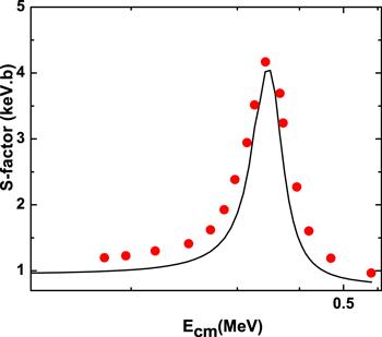
Figure 1. The solid line depicts the resonant s1/2 transition form Jπ = 1− to the bound states Jπ = 1+, 0+ and 1+ using only the PM. The filled circles shows the experimental data of [22]. |
There is another possible E1 transition that take place from the Jπ = 2− to the ground state Jπ = 3+ of 10B. This resonance does not have a significant contribution to the total radiative capture cross-section within the selected energy range, especially at zero energy. We accounted their non-resonance contribution. As a consequence, we consider the PM that describing the proton wave function in its continuum as a conventional Coulomb function in the d5/2 and d3/2 states. The d5/2 → p1/2 and d3/2 → p1/2 transitions may lead to a non-significant contribution to the total cross-section.
We also took into account the M1 transition from the continuum Jπ = 2+ at excitation energy Ex = 7.469 MeV and Γ = 65 keV [23] to the ground state Jπ = 3+ of 10B. We can not regenerate this result by PM. Therefore, we employed the R-matrix method equation (9 ) for the calculation of resonance cross-section. We took the radiative width Γγ from [24] while the total width Γ(E) from [23]. For the resonant transition computed by the R-matrix method the channel radius b = 5 fm was taken into consideration. Further, we considered the non-resonant transition of proton from the continuum to the ground state.
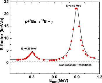
Adding up the outcomes of our calculations, as defined by the PM and R-matrix methods, the total S(0) is 1.307 keV·b, while the S(0) was 1.2 keV·b [4], 1.05 keV·b [8], and 4.3 keV·b [10]. We furthermore depicted the partial sum of all S-factors for 10B within the energy range (0–1.3) MeV in figure 2. The present result of S-factor coincides well with the experimental results both below, above and at the resonant positions 0.29 and 0.89 MeV. The result of χ2 test was 3.045. Further studies may give more insight in the study of 9Be(p, γ)10B within the framework of PM and R-matrix approach.
Figure 2. The solid line depicts the sum of resonant (s wave resonance peak at 0.29 MeV and p wave resonance peak at 0.89 MeV) and non-resonant (d wave Jπ = 2−) transitions using the PM and R-matrix approach. The dashed line shows the non-resonant transitions. The filled circle shows the experimental data [22]. |
4. Conclusion
For the computation of partial components of S-factors, we have used PM and R-matrix methods. We accounted for the multi-entrance channel radiative capture of proton by 9Be. Within the PM, the bound wave functions were obtained by modifying the Woods–Saxon potential. The PM approach was not only applied for ground state but also for the excited state wave functions. The model regenerates the existed measured data for (p, γ) reaction. There are certain cases, at high excitation energy (Ex), where the PM fails to regenerate the experimental data. We employed the R-matrix approach for such cases. Our model based results show that the present scheme is a reasonable approach for the radiative capture of proton by 9Be for multi-channel capture processes.