


1. Introduction
Using quantum matter as a working substance [1], a quantum heat engine (QHE) as its classical counterpart can transform heat to work. The QHE can fall into three categories, i.e., a four-stroke engine [2] , a two-stroke engine [3], and a continuous engine [4], and the Carnot and Otto engine belongs to the four-stroke engine category. The QHE model has been applied to many fields, such as laser [5], photocell [6] and photosynthesis [7]. The QHE has been realized in nitrogen-vacancy centers [8], nuclear magnetic resonance [9, 10], trapped ion [11], quasi-spin system [12] and impurity electron spin in a silicon tunnel field-effect transistor [13]. It is found that there is a trade-off relation between the power and efficiency of the engine [14], which attracts much attention on the finite time thermodynamics [15–18]. In classical thermodynamics, it is found that the C-A efficiency ${\eta }_{\mathrm{CA}}=1-\sqrt{{T}_{l}/{T}_{h}}$ is universal [19]. For QHE under certain conditions this C-A efficiency is also universal [20, 21]. We note that the QHE is an open quantum system, and as a result its state evolution can be described by a master equation. But for a non-adiabatic driven system the usual derivation of the Lindblad master equation is invalid [22], and this problem can be avoided in the quantum Otto heat engine.
One difference between the QHE and its corresponding classical counterpart is that the quantum information can be employed to increase the efficiency of the QHE [23, 24]. Szilárd shows that using classical information in a heat engine can extract work circularly from only one heat reservoir [25]. For the QHE it is also proposed that the information reservoir can be used to extract work from a single heat reservoir [26]. More generally the resource theory is used to study the thermodynamic process [27]. There are many proposals to utilize quantum information to drive the heat engine to surpass its classical counterpart [28–30]. Specifically it is shown that the indefinite causal order (ICO) is capable of effectively cooling a heat reservoir [31].
The definite causal order means that operations performed temporally follow one another, and inversely the ICO means that the order of the operations is indefinite. In resource theory, operations can be performed in ICO, which has been applied to the field of quantum information and other aspects [32–38]. One of the ICO is the quantum SWITCH, which can be implemented through coherent control by a quantum system. In quantum thermodynamics, Falce and Vedral have proposed a thermodynamic refrigeration cycle with an ICO [31], and then its unitary equivalent process has been achieved on a cloud quantum computer [39] and nuclear magnetic resonance system [40]. Recently this refrigerator has been explored with an optical quantum simulator [41]. Then there is an interesting question about the role of the ICO on the efficiency of the QHE.
In this paper, we study the influence of the ICO on the efficiency of an Otto engine. We first review what a ICO is, and then propose a model of an Otto engine with an ICO. Lastly we show that this Otto engine with ICO can be implemented with two trapped ions. In this model, we show that both the quasi-static efficiency and the efficiency at maximum power are much higher than the corresponding efficiency of a normal Otto heat engine.
2. The indefinite casual order
The effects of the heat reservoir on the work substance can be expressed in the Kraus representation as
$\begin{eqnarray}\varepsilon (\rho )=\sum _{i}{E}_{i}\rho {E}_{i}^{\dagger },\end{eqnarray}$
where $\left\{{E}_{i}\right\}$ is the Kraus operators and satisfies ${\sum }_{i}{E}_{i}^{\dagger }{E}_{i}=I$ [32, 33]. Here we consider that the control quantum system is a qubit, and correspondingly there are two kinds of Kraus operators Ei1 and Ej2, which describe the effect of the first kind and the second of the heat reservoirs, respectively. The ICO of the first and second kind operations can be implemented by a quantum SWICH through the control qubit, which can be described by $\begin{eqnarray}{W}_{{ij}}=| 0\rangle \langle 0{| }_{c}\otimes {E}_{i}^{2}{E}_{j}^{1}+| 1\rangle \langle 1{| }_{c}\otimes {E}_{j}^{1}{E}_{i}^{2}.\end{eqnarray}$
Obviously, when the control qubit is the state ${\left|0\right\rangle }_{c}$, the order is the first kind operation acting at first and then the second, and inversely the second kind acting at first and then the first kind if the control qubit is the state ${\left|1\right\rangle }_{c}$. The state after the quantum SWITCH is $\begin{eqnarray}{ \mathcal S }({\rho }_{c}\otimes \rho )=\sum _{i,j}{W}_{{ij}}({\rho }_{c}\otimes \rho ){W}_{{ij}}^{\dagger },\end{eqnarray}$
where the state of the work substance (control qubit) is ρ (ρc).Now we consider the interaction between the work substance and the heat reservoir. For simplicity, we assume that the work substance is also a qubit, whose Hamiltonian is $H=\tfrac{1}{2}\omega {\sigma }_{z}$ with ω being the transition frequency between these two levels, and σz being the Pauli operator. This work substance can exchange heat with a heat reservoir. Here for simplicity we assume that the effects of the reservoir on the work substance can be described by the following Lindblad master equation4 ) is equivalent to $\rho (t)\,={E}_{0}{\rho }_{0}{E}_{0}^{\dagger }+{E}_{1}{\rho }_{0}{E}_{1}^{\dagger }+{E}_{2}{\rho }_{0}{E}_{2}^{\dagger }+{E}_{3}{\rho }_{0}{E}_{3}^{\dagger }$.
$\begin{eqnarray}\displaystyle \frac{{\rm{d}}\rho ({t})}{d{t}}=-{\rm{i}}[{H},\rho ({t})]+{ \mathcal L }[\rho ({t})],\end{eqnarray}$
where the dissipator is ${ \mathcal L }[\rho (t)]=\tfrac{1}{2}\gamma (n+1)(2{\sigma }_{-}\rho {\sigma }_{+}-{\sigma }_{+}{\sigma }_{-}\rho $ $-\rho {\sigma }_{+}{\sigma }_{-})+\tfrac{1}{2}\gamma n(2{\sigma }_{+}\rho $ σ− − σ−σ+ρ − ρσ−σ+), γ is the damping rate, $n={\left({{\rm{e}}}^{{\hslash }\omega /{\kappa }_{{\rm{B}}}{T}}-1\right)}^{-1}$ is the mean number of bath quanta, and σ− = ∣0⟩⟨1∣ (σ+ = ∣1⟩⟨0∣) is the lowering (raising) operator. The solution of this master equation can be represented by the following Kraus operators ${E}_{0}=\sqrt{p}\left(\begin{array}{cc}1 & 0\\ 0 & \sqrt{1-\gamma ^{\prime} }\end{array}\right)$, ${E}_{1}=\sqrt{p}\left(\begin{array}{cc}0 & \sqrt{\gamma ^{\prime} }\\ 0 & 0\end{array}\right)$, ${E}_{2}=\sqrt{1-p}\left(\begin{array}{cc}\sqrt{1-\gamma ^{\prime} } & 0\\ 0 & 1\end{array}\right)$, ${E}_{3}=\sqrt{1-p}\left(\begin{array}{cc}0 & 0\\ \sqrt{\gamma ^{\prime} } & 0\end{array}\right)$, where $p=\tfrac{n}{1+2n}$, and $\gamma ^{\prime} =1-{{\rm{e}}}^{-\gamma (1+2n)t}$, and it can be easily checked that the state evolution governed by equation (3. A quantum Otto cycle with an ICO
In a quantum system the internal energy is defined as $U=\mathrm{Tr}[{H}\rho ({\rm{t}})]$, and its differential is $\mathrm{d}{U}=\mathrm{Tr}\rho \mathrm{d}H+\mathrm{Tr}H\mathrm{d}\rho $. The work and heat can be defined as $dW=\mathrm{Tr}\rho dH$ and $dQ=\mathrm{Tr}Hd\rho =\mathrm{Tr}H{ \mathcal L }[\rho ({t})]dt$ [42], respectively. Obviously the first law dU = dW + dQ is satisfied. In a finite time process the heat is obtained by integration
$\begin{eqnarray}Q={\int }_{0}^{{t}^{{\prime} }}TrH{ \mathcal L }[\rho ({t})]dt.\end{eqnarray}$
In the following the calculation is obtained in Bloch representation, i.e., the ρ is written as $\rho =\tfrac{1}{2}\left(\begin{array}{cc}1+z & x-\mathrm{iy}\\ x+\mathrm{iy} & 1-z\end{array}\right)$, and the initial state of work substance is expressed as ${x}_{0}=r\sin \theta \cos \phi $, ${y}_{0}=r\sin \theta \sin \phi $, and ${z}_{0}=r\cos \theta $.The Otto cycle consists of two isochoric strokes and two adiabatic strokes, as presented in figure 1. The first stroke is the isochoric cooling stroke, in which the heat is transferred from the work substance to the cold reservoir. In this stroke, the interaction between the work substance and two kind reservoirs is controlled by a control qubit, i.e., the heat transport in this stroke is achieved through the ICO operation. The third stroke is the isochoric heating strokes. In this stroke, the work substance contact with a hot reservoir, and heat is absorbed by the work substance. This stroke is the same as that in the usual Otto cycle. The second and the fourth strokes are two isentropic strokes, and the work is done by or on the work substance. In these two isentropic strokes, the work substance is isolated from the heat reservoir, and as a result there is no heat transferred.
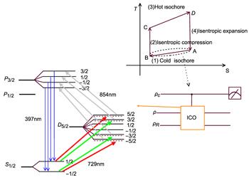
Figure 1. A schematic diagram of quantum Otto cycle based on two-level quantum system. The thermodynamic cycle consists of two isentropic strokes B → C (compression) and D → A (expansion) and two isochoric strokes A → B (cooling) and C → D (heating). The quantum circuit represents the cooling isochoric strokes, which is achieved by the quantum SWITCH followed by a measurement of the control qubit, where ρc, ρ and ρR denote the control qubit, work substance and reservoirs, respectively. Then the quantum SWITCH can be obtained through four sideband cooling as shown by the transition diagram. |
As only the isochoric cooling stroke of our Otto QHE is different from the usual Otto QHE, we will concentrate on this stroke. In this isochoric cooling strokes, two kinds of cold reservoirs are placed in an ICO by the quantum SWITCH, which reduce the heat transferred to them. Here and following we assume that these two kinds of reservoirs are the same. The initial state of the control qubit is set as ρc = ∣ψc⟩⟨ψc∣ with $| {\psi }_{c}\rangle =\sqrt{\alpha }| 0\rangle +\sqrt{1-\alpha }| 1\rangle $. The output state after the quantum SWITCH will be
$\begin{eqnarray}\begin{array}{l}{ \mathcal S }({\rho }_{c}\otimes \rho )=[\alpha | 0\rangle \langle 0{| }_{c}+(1-\alpha )| 1\rangle \langle 1{| }_{c}]\\ \otimes \,A+\sqrt{\alpha (1-\alpha )}[| 0\rangle \langle 1{| }_{c}+| 1\rangle \langle 0{| }_{c}]\otimes B,\end{array}\end{eqnarray}$
where $A=\left(\begin{array}{cc}{A}_{00} & {A}_{01}\\ {A}_{10} & {A}_{11}\end{array}\right)$ and $B=\left(\begin{array}{cc}{B}_{00} & {B}_{01}\\ {B}_{10} & {B}_{11}\end{array}\right)$ are the matrix of the Kraus operators acting on the work substance, with the elements being ${A}_{00}={{\rm{e}}}^{-2(1+2n){\gamma }_{1}{t}_{1}}(1+2{{\rm{e}}}^{2(1+2n){\gamma }_{1}{t}_{1}}n+{z}_{0}+2{{nz}}_{0})/(2+4n)$, ${A}_{01}=\tfrac{1}{2}{{\rm{e}}}^{-(1+2n){\gamma }_{1}{t}_{1}}({x}_{0}-{\rm{i}}{y}_{0})$, ${A}_{10}=\tfrac{1}{2}{{\rm{e}}}^{-(1+2n){\gamma }_{1}{t}_{1}}({x}_{0}+{\rm{i}}{y}_{0})$, ${A}_{11}={{\rm{e}}}^{-2(1+2n){\gamma }_{1}{t}_{1}}[2(1+n){{\rm{e}}}^{2(1+2n){\gamma }_{1}{t}_{1}}-(1+2n){z}_{0}-1]/(2+4n)$, ${B}_{00}=\tfrac{1}{2{\left(1+2n\right)}^{2}}\{2n(1+n)(1+{z}_{0}){{\rm{e}}}^{-(1+2n){\gamma }_{1}{t}_{1}}+{\left(1+n\right)}^{2}(1+{z}_{0})$ ${{\rm{e}}}^{-2(1+2n){\gamma }_{1}{t}_{1}}+n[-2\sqrt{{{\rm{e}}}^{-(1+2n){\gamma }_{1}{t}_{1}}}(1+2n)({z}_{0}-1)+2(1$ $+2n)({z}_{0}-1){\left({{\rm{e}}}^{-(1+2n){\gamma }_{1}{t}_{1}}\right)}^{3/2}+n(1+{z}_{0})]\}$, B01 = $\tfrac{1}{2{\left(1+2n\right)}^{2}}[n(1+n)+{{\rm{e}}}^{-2(1+2n){\gamma }_{1}{t}_{1}}n(1+n)+{{\rm{e}}}^{-(1+2n){\gamma }_{1}{t}_{1}}(1+2n\,+2{n}^{2})]({x}_{0}-{\rm{i}}{y}_{0})\mathrm{,}$ ${B}_{10}=\tfrac{1}{2{\left(1+2n\right)}^{2}}[n(1+n)+{{\rm{e}}}^{-2(1+2n){\gamma }_{1}{t}_{1}}n(1+n)+{{\rm{e}}}^{-(1+2n){\gamma }_{1}{t}_{1}}(1+2n+2{n}^{2})]({x}_{0}+{\rm{i}}{y}_{0})$, and ${B}_{11}=\tfrac{-1}{2{\left(1+2n\right)}^{2}}\{{{\rm{e}}}^{-2(1+2n){\gamma }_{1}{t}_{1}}{n}^{2}(-1+{z}_{0})+2{{\rm{e}}}^{-(1+2n){\gamma }_{1}{t}_{1}}n(1+n)$ $({z}_{0}-1)+{\left(1+n\right)}^{2}({z}_{0}-1)-2{\left({{\rm{e}}}^{-(1+2n){\gamma }_{1}{t}_{1}}\right)}^{3/2}({{\rm{e}}}^{(1+2n){\gamma }_{1}{t}_{1}}$ $-1)n(1+n)(1+{z}_{0})-2{\left({{\rm{e}}}^{-(1+2n){\gamma }_{1}{t}_{1}}\right)}^{3/2}({{\rm{e}}}^{(1+2n){\gamma }_{1}{t}_{1}}-1)$ ${\left(1+n\right)}^{2}(1+{z}_{0})\}$ (where we set the damping rate as γ1). After the quantum SWITCH, we make a measurement of the control qubit in the $\left\{| +{\rangle }_{c},| -{\rangle }_{c}\right\}$ basis, and obtain the final state of the work substance $\begin{eqnarray}\rho (t){=}_{c}\langle \pm | { \mathcal S }({\rho }_{c}\otimes \rho )| \pm {\rangle }_{c}.\end{eqnarray}$
This process is presented in figure 1. The temperature of the work substance at final time will be higher or lower than that of the heat reservoir depending on the measured state of the control qubit being ∣ + ⟩c or ∣ − ⟩c.Then, when the result state ∣ − ⟩c is measured, we can obtain the reduced density matrix of the work substance at the final time t1 of isochoric cooling stroke from equations (4 ) and (8 ). Correspondingly, the heat transferred from the work substance into the cold reservoirs is
$\begin{eqnarray}{Q}_{l}={\int }_{0}^{{t}_{1}}\mathrm{Tr}H{\dot{\rho }}_{l}(t)\mathrm{dt},\end{eqnarray}$
and the work required to erase the control qubit (determined by Landauer principle) is $\begin{eqnarray}{W}_{d}={\kappa }_{B}{T}_{l}S,\end{eqnarray}$
where $S=-\mathrm{Tr}[{\rho }_{c}({{\rm{t}}}_{1})\mathrm{ln}{\rho }_{c}({{\rm{t}}}_{1})]$ here is the entropy of the control qubit at the final time t1.In the second and fourth strokes, there is no heat transferred and the work is equal to the change of the internal energy. For comparison with the normal Otto engine we consider the work done quasi-statically in these two strokes. The work in a quasi-static adiabatic process is ${W}^{\mathrm{adi}}=\sum {p}_{j}({E}_{j}^{f}-{E}_{j}^{i})$, with the probability ${p}_{j}=\tfrac{1}{{Z}^{i}}\exp [-{E}_{j}^{i}/({\kappa }_{B}T)]$, Eji (Ejf) being the j-th eigenvalue of the initial (final) Hamiltonian, and Zi = ∑j $\exp [-{E}_{j}^{i}/({\kappa }_{B}T)]$ being the partition function. Correspondingly the work in a quasi-static Otto engine is ${W}_{T}^{\mathrm{adi}}\,=-({W}_{B}^{\mathrm{adi}}+{W}_{D}^{\mathrm{adi}})$, with ${W}_{B}^{\mathrm{adi}}=\sum {p}_{j}({E}_{j}^{C}-{E}_{j}^{B})$ and ${W}_{D}^{\mathrm{adi}}\,=\sum {p}_{j}({E}_{j}^{A}-{E}_{j}^{D})$.
In the third stroke, the work substance is interacted with the hot reservoirs with the temperature Th, and its state denoted as ρh can be obtained by solving the equation (4 ) (the damping rate is supposed to be γ2). Here we assume that the duration of the interaction time is t2. As the work substance is isolated from the heat reservoir in the second and fourth strokes, it means that the initial (final) entropy of the first stroke is equal to the final (initial) entropy of the third stroke. We will use this property to determine the duration time t2. As a result, the heat transferred into the work substance from the hot reservoirs is
$\begin{eqnarray}{Q}_{h}={\int }_{0}^{{t}_{2}}\mathrm{Tr}H{\dot{\rho }}_{h}(t)\mathrm{dt}.\end{eqnarray}$
Similarly the heat in the corresponding quasi-static process is ${Q}_{h}^{\mathrm{adi}}=\sum {E}_{j}^{A}({p}_{j}^{A}-{p}_{j}^{D})$. Correspondingly the efficiency in our model can be calculated as $\begin{eqnarray}\eta =\displaystyle \frac{{Q}_{h}+{Q}_{l}-{W}_{d}}{{Q}_{h}}.\end{eqnarray}$
It has been shown that the efficiency of a normal Otto heat engine at maximum power is [43] $\begin{eqnarray}{\eta }_{\mathrm{EMP}}=\displaystyle \frac{2{\eta }^{\mathrm{adi}}}{3-{\eta }^{\mathrm{adi}}},\end{eqnarray}$
where the efficiency of the corresponding qua-sistatic Otto heat engine is ${\eta }^{\mathrm{adi}}=\tfrac{{W}_{T}^{\mathrm{adi}}}{{Q}_{h}^{\mathrm{adi}}}$.4. Performance of the heat engine
Here we propose a scheme to achieve our Otto heat engine in trapped ions. We assume that there are two trapped 40Ca† ions in a linear trap with one being a control qubit and another being work substance, and its energy levels are shown in figure 1. Here we assume that there is a magnetic field to split the Zeeman sublevels, which can be coupled individually through lasers with different frequency. Both the work substance and control qubit are encoded in the Zeeman qubit, i.e., $\left|0\right\rangle ={\left|0\right\rangle }_{c}=\left|{4}^{2}{S}_{1/2},{m}_{J}=-1/2\right\rangle $ and $\left|1\right\rangle ={\left|1\right\rangle }_{c}=\left|{4}^{2}{S}_{1/2},{m}_{J}=+1/2\right\rangle $, as shown in figure 1. The heat reservoir can be achieved though the technique of reservoir engineering. For hot reservoir it can be achieved through RF noise generator as achieved in [44]. The cold reservoir can be implemented by applying the 729 nm and 854 nm lasers to the control qubit, which can achieve the sideband cooling of the center of mass mode. If we add another 729 nm laser to the work substance, then we can couple it to the center of mass mode, which in turn result an indirect interaction between the work substance and the cold reservoir, and the master equation of this system composed by the center of mass mode and the work substance is4 ) [45].
$\begin{eqnarray}{\dot{\rho }}_{\mathrm{mw}}=-i\left[{H}_{\mathrm{mw}},{\rho }_{\mathrm{mw}}\right]+{\rm{\Gamma }}({\rho }_{\mathrm{mw}}),\end{eqnarray}$
where the density matrix of the composed system is ρmw, ${H}_{\mathrm{mw}}=\tfrac{1}{2}\omega {\sigma }_{z}+\nu {a}^{\dagger }a+{\rm{\Omega }}$ (σ−a† + σ+a) is its Hamiltonian with ω being the transition frequency of the work substance, ν (a† and a) being the frequency (the creation and annihilation operators) of the center of mass mode, Ω being the effective coupling strength between the work substance and the center of mass mode, ${\rm{\Gamma }}(\rho )=-\tfrac{1}{2}{\text{}}ϝ(n+1)({a}^{\dagger }a{\rho }_{\mathrm{mw}}-2a{\rho }_{\mathrm{mw}}{a}^{\dagger }+{\rho }_{\mathrm{mw}}{a}^{\dagger }a)$ $-\tfrac{1}{2}{\text{}}ϝn({{aa}}^{\dagger }{\rho }_{\mathrm{mw}}-2{a}^{\dagger }{\rho }_{\mathrm{mw}}a+{\rho }_{\mathrm{mw}}{{aa}}^{\dagger })$ being the dissipator,$ϝ$ being the cooling rate, and n being the average photon of the reservoir. We assume that the coupling strength between the reservoir and work substance γ = 4Ω2/$ϝ$ is weak compared with rate of cooling. Under this condition the variable of the center of mass mode can be eliminated adiabatically, and as a result the state evolution of the work substance is governed by the equation (We show how to implement the quantum SWITCH in our trapped ions. When the control qubit is in state ${\left|0\right\rangle }_{c}$, we apply the 729 nm and 854 nm lasers (denoted as L0l) to achieve the sideband cooling through the trajectory ${\left|0\right\rangle }_{c}\to {\left|{3}^{2}{D}_{5/2},{m}_{J}=-5/2\right\rangle }_{c}\to {\left|{4}^{2}{P}_{3/2},{m}_{J}=-3/2\right\rangle }_{c}$. Then we shut down the L0l , and simultaneously apply another 729 nm and 854 nm lasers (denoted as ${L}_{0}^{r}$) to achieve the sideband cooling through the trajectory ${\left|0\right\rangle }_{c}\to {\left|{3}^{2}{D}_{5/2},{m}_{J}=-3/2\right\rangle }_{c}\to {\left|{4}^{2}{P}_{3/2},{m}_{J}=-1/2\right\rangle }_{c}$. If the intensities or pulse lengths of the L0l and L0r are different, then these two cooling processes are also different. Being similar as the cases of the control qubit being state ${\left|0\right\rangle }_{c}$, when the control qubit is in state ${\left|1\right\rangle }_{c}$, we can achieve two sideband cooling through two pairs of 729 nm and 854 nm lasers, i.e., ${L}_{1}^{r}$ through the trajectory ${\left|1\right\rangle }_{c}\to {\left|{3}^{2}{D}_{5/2},{m}_{J}=3/2\right\rangle }_{c}\to {\left|{4}^{2}{P}_{3/2},{m}_{J}=1/2\right\rangle }_{c}$ and then L1l through the trajectory ${\left|1\right\rangle }_{c}\to {\left|{3}^{2}{D}_{5/2},{m}_{J}=5/2\right\rangle }_{c}\to {\left|{4}^{2}{P}_{3/2},{m}_{J}=3/2\right\rangle }_{c}$. We can tune the intensities and pulse lengths of the lasers L1l (L1r ) to be equal to that of the L0l (L0r), which will induce the operation induced by L1l (L1r) to be identical to that by the L0l (L0r). In other words we can obtain two kinds of reservoirs. As a result, when the control qubit is in a superposition state, we implement the quantum SWITCH. As mentioned above, we will further set these two kinds of reservoirs as being identical.
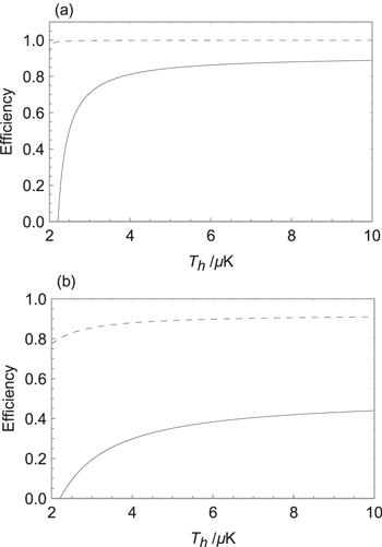
Now we present our calculation in this system. In our calculation, we fix the duration time t1 of the quantum SWITCH, which should assure that the heat is released from the work substance to the cold reservoirs. Then we change the interaction time t2 between the work substance and the hot reservoir to obtain the maximum (or minimum) power and the corresponding time. With these two times we can obtain the quasi-static efficiency (here corresponding to minimum power) and the efficiency at maximum power. To show the advantage of the ICO, we compare our results with the efficiency of the normal Otto engine. In figure 2(a) we compare the quasi-static efficiency. It shows that our efficiency is much larger than that of the normal Otto engine and can reach unit one. In figure 2(b) we compare the efficiency at maximum power. Being similar as the case of the quasi-static efficiency, our efficiency at maximum power is also better than that of the normal Otto engine. These enhancement of the efficiency can be attributed to two reasons. The first one is the non-equilibrium of the cold reservoir. As the control qubit should be included in the cold reservoir, and correspondingly the state of this enlarged heat reservoir is no longer equilibrium. We note that the ICO is, essentially, a series of conditional operations, and as a result, the second one is the measurement of the control qubit, as shown in Maxwell demon that the measurement can enhance the efficiency of heat engine [46, 47].
Figure 2. The efficiency versus the temperature of the hot reservoir Th. (a) Comparison of the quasi-static efficiency between our heat engine and the normal Otto heat engine, where the dashed and solid curves are the quasi-static efficiency of our engine and of the normal Otto heat engine, respectively. (b) Comparison of the efficiency at maximum power between our heat engine and a normal Otto heat engine, where the dashed and solid curves are the efficiency η and ηEMP, respectively. The parameters are $\alpha =\tfrac{1}{2}$, ω = 2π × 50 KHz, γ1 = 2π × 2 KHz, γ2 = 2π × 2 KHz, θ = 3, φ = π/2, r = 0.5, and Tc = 1 μK. |
5. Conclusion
In this paper, we proposed a model of an Otto engine with the ICO. Then we show how to achieve this engine with two trapped ions. With this model we studied the effect of the ICO in the Otto cycle on the performance of the heat engine, and found that the efficiency of the heat engine could be improved by the ICO, i.e., the efficiency at maximum power can be significantly improved over the corresponding efficiency of the normal Otto engine, and the quasi-static efficiency can also greatly exceed that of the normal Otto engine and may be close to one.