Welcome to visit Communications in Theoretical Physics,
Quantum Physics and Quantum Information

Entanglement witnesses of four-qubit tripartite separable quantum states

  • Miao Xu(徐淼) 1 ,
  • Wei-Feng Zhou(周伟峰) 1 ,
  • Feng Chen(陈峰) 1 ,
  • Li-Zhen Jiang(蒋丽珍) , 1, ∗∗ ,
  • Xiao-Yu Chen(陈小余) 2
Expand
  • 1College of Information and Electronic Engineering, Zhejiang Gongshang University, Hangzhou 310018, China
  • 2School of Information & Electrical Engineering, Zhejiang University City College, Hangzhou 310015, China

∗∗ Author to whom any correspondence should be addressed.

Received date: 2021-10-15

  Revised date: 2021-12-01

  Accepted date: 2021-12-03

  Online published: 2022-03-22

Supported by

*National Natural Science Foundation of China(61871347)

Copyright

© 2022 Institute of Theoretical Physics CAS, Chinese Physical Society and IOP Publishing

Abstract

A quantum entangled state is easily disturbed by noise and degenerates into a separable state. Compared to the entanglement with bipartite quantum systems, less progress has been made for the entanglement with multipartite quantum systems. For tripartite separability of a four-qubit system, we propose two entanglement witnesses, each of which corresponds to a necessary condition of tripartite separability. For the four-qubit GHZ state mixed with a W state and white noise, we prove that the necessary conditions of tripartite separability are also sufficient at W states side.

Cite this article

Miao Xu(徐淼) , Wei-Feng Zhou(周伟峰) , Feng Chen(陈峰) , Li-Zhen Jiang(蒋丽珍) , Xiao-Yu Chen(陈小余) . Entanglement witnesses of four-qubit tripartite separable quantum states[J]. Communications in Theoretical Physics, 2022 , 74(3) : 035102 . DOI: 10.1088/1572-9494/ac3fb1

1. Introduction

Quantum entanglement [1] as an extremely crucial resource [2] has potential applications for quantum computation and quantum communication. A quantum state is only known as separable if it can be generated by local operations and classical communications (LOCC) only, otherwise it is entangled. It is particularly significant to have a criterion that can systematically determine whether a given quantum state is entangled or separable. In 1996, Peres first put forward positive partial transition (PPT) [3] criterion, later, Horodecki proved that PPT criterion is not only necessary but also sufficient in the ${{ \mathcal H }}_{2}\otimes {{ \mathcal H }}_{2}$ and ${{ \mathcal H }}_{2}\otimes {{ \mathcal H }}_{3}$ systems. For example, a quantum state ρ has elements ρμκ,νι = ⟨μ∣⟨κρν⟩∣ι⟩, if its partial transposition ${\rho }^{{{\rm{T}}}_{{A}}}$(with ${\rho }_{\mu \kappa ,\nu \iota }^{{{\rm{T}}}_{{A}}}={\rho }_{\nu \kappa ,\mu \iota }$) is positive, the state is separable [4]. However, in some high dimensional quantum state systems, such as ${{ \mathcal H }}_{3}\otimes {{ \mathcal H }}_{3}$ and ${{ \mathcal H }}_{2}\otimes {{ \mathcal H }}_{4}$, the transposition of some entangled state is also positive [5]. It shows that PPT criterion may no longer be sufficient for the separability of high dimensional and multipartite quantum states. Another separable criterion, the computable cross-norm or realignment (CCNR) criterion which can detect some other entangled states is regarded as a complement [6] to PPT criterion. Range criterion [7] and some other criteria had also been proposed. However, there is an obvious defect within the range criterion that the density matrix of the quantum state and its partial transposition are generally full rank in a noise environment,which makes the criterion no longer applicable. Quantum Fisher information (QFI) [810] has been used in the detection of the entanglement and the k-nonseparability of multipartite quantum systems. Entanglement witness [11] is also widely used and appropriate for multipartite systems in entanglement detection [1217]. Theoretically, an entanglement witness exists which can be a sufficient and necessary condition for detecting entanglement. The entanglement witness is essentially an observable Hermitian operator $\hat{W}$, we have $\mathrm{Tr}[\hat{W}{\rho }_{s}]\geqslant 0$ for all separable quantum state ρs and there is at least an entangled state ρe such that $\mathrm{Tr}[\hat{W}{\rho }_{e}]\lt 0$, we assert that the state ρe is witnessed by $\hat{W}$ [18]. Then the task of detecting entanglement is transformed into searching for an entanglement witness.
Compared to the entanglement with bipartite quantum systems, less progress has been made for the entanglement with multipartite quantum systems [1922]. When we study the entanglement with multipartite quantum systems, besides the full separability [23, 24] or full entanglement of all particles, the partial separability [25] has also attracted much attention. In the finite dimensional composite Hilbert space ${ \mathcal H }={{ \mathcal H }}_{1}\otimes ...\otimes {{ \mathcal H }}_{n}$, we divide the index set ${ \mathcal J }=\{1,\ldots ,n\}$ into m parts and denote the partition as ${ \mathcal I }=\{{{ \mathcal I }}_{1},\ldots ,{{ \mathcal I }}_{m}\}$, a quantum state ${\sigma }_{{ \mathcal I }}$ is separable with respect to the partition ${ \mathcal I }$ if it can be written as follows:
$\begin{eqnarray}{\sigma }_{{ \mathcal I }}=\sum _{i}{q}_{i}| {\psi }_{{{ \mathcal I }}_{1}}^{(i)}\rangle \langle {\psi }_{{{ \mathcal I }}_{1}}^{(i)}| \otimes ...\otimes | {\psi }_{{{ \mathcal I }}_{m}}^{(i)}\rangle \langle {\psi }_{{{ \mathcal I }}_{m}}^{(i)}| ,\end{eqnarray}$
where qi is a classical probability distribution, $| {\psi }_{{{ \mathcal I }}_{j}}^{(i)}\rangle $ is the pure state in the subset of ${{ \mathcal I }}_{j}$. Further, if the state σ is in the form of
$\begin{eqnarray}\sigma =\sum _{{ \mathcal I }:| { \mathcal I }| =k}{q}_{{ \mathcal I }}^{{\prime} }{\sigma }_{{ \mathcal I }},\end{eqnarray}$
we call it k-separable [26, 27], where $| { \mathcal I }| $ is the number of elements of set ${ \mathcal I }$, and ${q}_{{ \mathcal I }}^{{\prime} }$ is a classical probability distribution. In the four-qubit triseparable system, if qubits 1, 2, 3, 4 exist, we divide the first and second qubit into the first and second part respectively, and the third and fourth qubits as the third part, which is denoted as ∣1∣2∣34∣. Consequently the pure product state is
$\begin{eqnarray}| {{\rm{\Psi }}}_{s}\rangle =| {{\rm{\Psi }}}_{1}\rangle \otimes | {{\rm{\Psi }}}_{2}\rangle \otimes | {{\rm{\Psi }}}_{34}\rangle .\end{eqnarray}$
In computational basis, a single qubit pure state is
$\begin{eqnarray}\begin{array}{l}| {{\rm{\Psi }}}_{j}\rangle ={c}_{j}| 0\rangle +{s}_{j}{{\rm{e}}}^{{\rm{i}}{\varphi }_{j}}| 1\rangle \\ \quad =\displaystyle \frac{1}{\sqrt{1+| {\xi }_{j}{| }^{2}}}\left(| 0\rangle +{\xi }_{j}| 1\rangle \right),\end{array}\end{eqnarray}$
where ${c}_{j}=\cos (\tfrac{{\theta }_{j}}{2})$, ${s}_{j}=\sin (\tfrac{{\theta }_{j}}{2})$, ${\xi }_{j}={{\rm{e}}}^{{\rm{i}}{\varphi }_{j}}\tan \tfrac{{\theta }_{j}}{2}$, (j = 1, 2).
The paper is organized as follows. In sections 2 and 3 we propose two entanglement witnesses, respectively, each of which corresponds to a necessary condition of tripartite separability for any four-qubit quantum state. We conclude in section 4. GHZ states [28] and W states [29] as the common multipartite entangled states are often used in quantum information processing. Additive white noise has been introduced to describe the effect of the environment on a quantum state. The density matrix of a four-qubit GHZ state mixed with a W state and white noise (denote as noisy GHZ-W state) is
$\begin{eqnarray}\rho =p| \mathrm{GHZ}\rangle \langle \mathrm{GHZ}| +q| {\rm{W}}\rangle \langle {\rm{W}}| +\displaystyle \frac{1-p-q}{16}{I}_{16},\end{eqnarray}$
where (p, q, 1 − pq) represents the probability distribution. I16/16 represents white noise, where ${I}_{16}={\sum }_{i=0}^{4}{D}_{i}$ is the 16 × 16 identity matrix, with Di = ∑k∣=ik⟩⟨k∣ in which k = k1k2k3k4 is a binary sequence vector and ∣k∣ is the Hamming weight of vector k. The four-qubit GHZ state is $| \mathrm{GHZ}\rangle =\tfrac{1}{\sqrt{2}}(| 0000\rangle +| 1111\rangle )$, and the four-qubit W state is $| {\rm{W}}\rangle =\tfrac{1}{2}{\sum }_{| k| =1}| k\rangle $. For a noisy GHZ-W state, we will prove that the two necessary conditions of tripartite separability are also sufficient for the parameter interval of ${\rm{\Theta }}=\arctan (\tfrac{p}{q})\in [0,0.080401\pi ]$ and [0.080401π, 0.11628π] respectively.

2. The first entanglement witness

We propose the first entanglement witness ${\hat{W}}_{1}$. We arrange the order of four qubit computation basis ∣k⟩ with the ascending order of ∣k∣. In such a basis, the 16 × 16 matrix ${\hat{W}}_{1}$ is defined as
$\begin{eqnarray}{\hat{W}}_{1}=\left[\begin{array}{cccc}\displaystyle \frac{4}{3d} & & & \\ & {E}_{1} & & \\ & & \displaystyle \frac{d}{3}{E}_{2} & \\ & & & \ddots \end{array}\right],\end{eqnarray}$
where d > 0, the E1 represents the 4th order matrix $\left[\begin{array}{cccc}1 & -1 & -1 & -1\\ -1 & 1 & -1 & -1\\ -1 & -1 & 1 & -1\\ -1 & -1 & -1 & 1\end{array}\right],$ and the E2 represents the 6th order matrix $\left[\begin{array}{llllll}4 & 1 & 1 & 1 & 1 & 4\\ 1 & 4 & 1 & 1 & 4 & 1\\ 1 & 1 & 4 & 4 & 1 & 1\\ 1 & 1 & 4 & 4 & 1 & 1\\ 1 & 4 & 1 & 1 & 4 & 1\\ 4 & 1 & 1 & 1 & 1 & 4\end{array}\right],$ and the remaining elements not identified are zeros.

For any four-qubit quantum state ρ, a necessary criterion of tripartite separability is $\mathrm{Tr}\left[\rho {\hat{W}}_{1}\right]\geqslant 0$.

Under the partition $| 1| 2| 34| $, the pure state is shown in equation (3), we define ${\widetilde{W}}_{1}=\langle {{\rm{\Psi }}}_{1}| \langle {{\rm{\Psi }}}_{2}| {\hat{W}}_{1}| {{\rm{\Psi }}}_{1}\rangle | {{\rm{\Psi }}}_{2}\rangle $, then the validity of ${\hat{W}}_{1}$ as a witness is equivalent to the positive semi-definite of ${\widetilde{W}}_{1}$. The 4 × 4 matrix ${\widetilde{W}}_{1}$ is

$\begin{eqnarray}{\widetilde{W}}_{1}=\displaystyle \frac{1}{\sqrt{{N}_{1}{N}_{2}}}\left[\begin{array}{cccc}A & {B}^{* } & {B}^{* } & {E}^{* }\\ B & C & D & {H}^{* }\\ B & D & C & {H}^{* }\\ E & H & H & F\end{array}\right],\end{eqnarray}$
where ${N}_{1}={\left(1+| {\xi }_{1}{| }^{2}\right)}^{2}$, ${N}_{2}={(1+| {\xi }_{2}{| }^{2})}^{2}$, and $A=\tfrac{4}{3d}\,+| {\xi }_{1}-{\xi }_{2}{| }^{2}+\tfrac{4d}{3}| {\xi }_{1}{\xi }_{2}{| }^{2}$,
$B=-({\xi }_{1}+{\xi }_{2})+\tfrac{d}{3}{\xi }_{1}{\xi }_{2}({\xi }_{1}^{* }+{\xi }_{2}^{* })$,
$C=1+\tfrac{4d}{3}(| {\xi }_{1}{| }^{2}+| {\xi }_{2}{| }^{2})+\tfrac{d}{3}({\xi }_{1}{\xi }_{2}^{* }+{\xi }_{1}^{* }{\xi }_{2})$,
$D=-1\,+\tfrac{d}{3}(| {\xi }_{1}{| }^{2}+| {\xi }_{2}{| }^{2})+\tfrac{4d}{3}({\xi }_{1}{\xi }_{2}^{* }+{\xi }_{1}^{* }{\xi }_{2})$,
$E=\tfrac{4d}{3}{\xi }_{1}{\xi }_{2}$, $F=\tfrac{4d}{3}$, $H=\tfrac{d}{3}({\xi }_{1}+{\xi }_{2})$. If the following matrix is positive semi-definite:
$\begin{eqnarray}{\widetilde{W}}_{1}^{{\prime} }=\left[\begin{array}{ccc}A & \sqrt{2}{B}^{* } & {E}^{* }\\ \sqrt{2}B & C+D & \sqrt{2}{H}^{* }\\ E & \sqrt{2}H & F\end{array}\right],\end{eqnarray}$
${\widetilde{W}}_{1}$ is also positive semi-definite. In fact, ${\tilde{W}}_{1}\cdot (\alpha ,\beta ,\beta ,\gamma {)}^{{\rm{T}}}=0$ is equivalent to ${\tilde{W}}_{1}^{{\prime} }\cdot (\alpha ,\sqrt{2}\beta ,\gamma {)}^{{\rm{T}}}=0$. The determinant is $\det (\widetilde{W}^{{\prime} }_{1})=2{d}^{2}| {\xi }_{1}^{2}-{\xi }_{2}^{2}{| }^{2}$. Obviously, the matrix $\widetilde{W}^{{\prime} }_{1}$ is always positive semi-definite, and we conclude the ${\widetilde{W}}_{1}$ is also positive semi-definite, so ${\hat{W}}_{1}$ is a valid entanglement witness.

A necessary condition of tripartite separability for a noisy GHZ-W state is

$\begin{eqnarray}8(1-p-q)(1-p+7q)\geqslant 3{\left(1-9p-q\right)}^{2}.\end{eqnarray}$

According to Theorem 1, we can obtain the result for a noisy GHZ-W state as follows:

$\begin{eqnarray}\begin{array}{l}\mathrm{Tr}[\rho {\hat{W}}_{1}]=\displaystyle \frac{2q+4c}{3d}+4c+8{cd}-2p\\ \quad \geqslant 4\sqrt{\displaystyle \frac{{qc}+2{c}^{2}}{3}}+4c-2p\geqslant 0,\end{array}\end{eqnarray}$
where $c=\tfrac{1-p-q}{16}$. Then condition (9) follows, and it is displayed with a cyan solid line in figure 1.

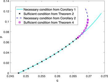
Figure 1. Necessary and/or sufficient criteria for the triseparability of state $\rho =p| \mathrm{GHZ}\rangle \langle \mathrm{GHZ}| +q| {\rm{W}}\rangle \langle {\rm{W}}| +\tfrac{1-p-q}{16}{I}_{16}$.

For a noisy GHZ-W state, the necessary criterion of tripartite separability in corollary 1 is also sufficient in the parameter interval of ${\rm{\Theta }}\in [0,0.080401\pi ]$.

We try to construct a quantum state ${\rho }_{s}=| {{\rm{\Psi }}}_{s}\rangle \langle {{\rm{\Psi }}}_{s}| $ which meets $\mathrm{Tr}[\hat{W}{\rho }_{s}]=0$ if we obtain an entanglement witness $\hat{W}$, hence we can get the boundary hypersurface distinguishing entangled states from separable states. We then construct a triseparable state using the eigenvectors corresponding to zero eigenvalues of some matrix derived from entanglement witness. In other words, the state which we used to construct the tripartite separable states in the boundary of tripartite separable state set should satisfy $\langle {{\rm{\Psi }}}_{s}| \hat{W}| {{\rm{\Psi }}}_{s}\rangle =0$. At $| {\rm{W}}\rangle $ states side of a noisy GHZ-W state, we construct triseparable states with type ${\rm{I}}:{\xi }_{1}={\xi }_{2}$ and type $\mathrm{II}:{\xi }_{1}=-{\xi }_{2}$, then mix the constructed states in order to offset the off diagonal elements except $| {\rm{W}}\rangle $ state and $| \mathrm{GHZ}\rangle $ state. The process is mainly divided into the following three steps:

Step 1. Construct triseparable states. In the case of type I and type II, we use a unitary matrix U = diag(e−iφ, 1, eiφ) to operate on ${\widetilde{W}}_{1}^{{\prime} }$ (see (8)), let ${\widetilde{W}}_{1}^{{\prime\prime} }={U}^{\dagger }{\widetilde{W}}_{1}^{{\prime} }U$. We try to get the value of V when ${\widetilde{W}}_{1}^{{\prime\prime} }V=0$, with $V={\left(\alpha ,\sqrt{2}\beta ,\gamma \right)}^{{\rm{T}}}$. Surely, it has also ${\widetilde{W}}_{1}^{{\prime} }{UV}=0$, with ${UV}={\left(\alpha {{\rm{e}}}^{-{\rm{i}}\varphi },\sqrt{2}\beta ,\gamma {{\rm{e}}}^{{\rm{i}}\varphi }\right)}^{{\rm{T}}}$ which is the eigenvector corresponding to zero eigenvalue of ${\widetilde{W}}_{1}^{{\prime} }$. Under the partition ∣1∣2∣34∣, the pure product state (see (3)) is shown as follows:
$\begin{eqnarray}\begin{array}{l}| {{\rm{\Psi }}}_{s}\rangle =({c}_{1}| 0\rangle +{s}_{1}{{\rm{e}}}^{{\rm{i}}{\varphi }_{1}}| 1\rangle )\otimes ({c}_{2}| 0\rangle +{s}_{2}{{\rm{e}}}^{{\rm{i}}{\varphi }_{2}}| 1\rangle )\\ \quad \otimes [\alpha {{\rm{e}}}^{-{\rm{i}}\varphi }| 00\rangle +\beta (| 01\rangle +| 10\rangle )+\gamma {{\rm{e}}}^{{\rm{i}}\varphi }| 11\rangle ].\end{array}\end{eqnarray}$
For the type I, there is ξ1 = ξ2 := ξeiφ , with $\xi =\tan \tfrac{\theta }{2}$, θ ∈ [0, π], φ ∈ [0, 2π], correspondingly, the quantum state is ${\rho }_{| 1| 2| 34| }=\tfrac{1}{4}{\sum }_{m=0}^{3}\left|{{\rm{\Psi }}}_{s}(\theta ,\varphi =\tfrac{(2m+1)\pi }{4})\right\rangle \left\langle \cdot \right|$. It is worth noting that we simplify ∣$\Psi$⟩⟨$\Psi$∣ to ∣$\Psi$⟩⟨ · ∣.
For the type II, there is ξ1 = − ξ2 := ηeiφ , with $\eta =\tan \tfrac{{\theta }^{{\prime} }}{2}$, φ2φ1 = π, the quantum state is now ${\rho }_{| 1| 2| 34| }^{{\prime} }\,=\tfrac{1}{4}{\sum }_{m=0}^{3}\left|{{\rm{\Psi }}}_{s}({\theta }^{{\prime} },\varphi =\tfrac{2m\pi }{4})\right\rangle \left\langle \cdot \right|$. It notes that the different values of φ are used in the above cases. One of the reasons is that the result should not be complex after discrete summation. The other is to ensure that those off diagonal elements except ∣W⟩ state and ∣GHZ⟩ state can be eliminated after mixing the triseparable states with suitable proportion. After summing the density matrices of all partitions and averaging the result, we can obtain the final density matrix of the triseparable state, it is
$\begin{eqnarray}\begin{array}{l}\rho =\displaystyle \frac{1}{12}\left({\rho }_{| 1| 2| 34| }+{\rho }_{| 2| 1| 34| }+{\rho }_{| 3| 4| 12| }+{\rho }_{| 4| 3| 12| }\right.\\ +{\rho }_{| 2| 4| 13| }+{\rho }_{| 4| 2| 13| }+{\rho }_{| 2| 3| 14| }+{\rho }_{| 3| 2| 14| }\\ \left.+{\rho }_{| 1| 4| 23| }+{\rho }_{| 4| 1| 23| }+{\rho }_{| 1| 3| 24| }+{\rho }_{| 3| 1| 24| }\right).\end{array}\end{eqnarray}$
In the type I and type II, the density matrices are ρI and ρII respectively, where ρI (ρII is similar) can be written as
$\begin{eqnarray}\begin{array}{l}{\rho }_{{\rm{I}}}={C}_{{\mathrm{GHZ}}_{{\rm{I}}}}\cdot | \mathrm{GHZ} \rangle \langle \cdot | +{C}_{{{\rm{W}}}_{{\rm{I}}}}\cdot | {\rm{W}} \rangle \langle \cdot | +{C}_{{{\rm{D}}}_{42{\rm{I}}}}\cdot | {{\rm{D}}}_{42} \rangle \langle \cdot | \\ \\ +{C}_{{\bar{{\rm{W}}}}_{{\rm{I}}}}\cdot | \bar{{\rm{W}}} \rangle \langle \cdot | +{C}_{{\bar{{\rm{D}}}}_{42{\rm{I}}}}\cdot {\rho }_{{\bar{{\rm{D}}}}_{42}}+\displaystyle \sum _{i=0}^{4}{C}_{i{\rm{I}}}\cdot {D}_{i},\\ \end{array}\,\end{eqnarray}$
where ${C}_{{\mathrm{GHZ}}_{{\rm{I}}}}$ means the coefficient of the ∣GHZ⟩ state in type I, and so on. $| \overline{{\rm{W}}}\rangle =\tfrac{1}{2}{\sum }_{| k| =3}| k\rangle $ is the qubit flip of the four-qubit ∣W⟩ state. $| {{\rm{D}}}_{42}\rangle =\tfrac{1}{\sqrt{6}}{\sum }_{| k| =2}| k\rangle $ is the Dicke state. And ${\rho }_{{\overline{{\rm{D}}}}_{42}}$ is
$\begin{eqnarray}\begin{array}{rcl}{\rho }_{{\bar{{\rm{D}}}}_{42}} & = & | 0011 \rangle \langle 1100| +| 0101 \rangle \langle 1010| +| 0110 \rangle \langle 1001| \\ & & \\ & & +| 1001 \rangle \langle 0110| +| 1010 \rangle \langle 0101| +| 1100 \rangle \langle 0011| .\\ & & \end{array}\,\end{eqnarray}$
Step 2. Offset the off diagonal elements except ∣W⟩ state and ∣GHZ⟩ state. In the case of type I, let $\delta =\tfrac{1}{3d}$, the values of (α, β, γ) in equation (11) are
$\begin{eqnarray}\begin{array}{rcl}\alpha & = & \sqrt{\displaystyle \frac{{\xi }^{2}}{{\xi }^{2}+2{\delta }^{2}+{\left(\delta +{\xi }^{2}\right)}^{2}{\xi }^{2}}},\\ \beta & = & \displaystyle \frac{\delta \alpha }{\xi }\quad \mathrm{and}\quad \gamma =-(\delta +{\xi }^{2})\alpha .\end{array}\end{eqnarray}$
In the case of type II, there are ${\alpha }^{{\prime} }={\gamma }^{{\prime} }=0$ and ${\beta }^{{\prime} }=\tfrac{1}{\sqrt{2}}$. Then we return to step 1 to construct states ρI and ρII. It shows that ${C}_{{{\rm{D}}}_{42{\rm{I}}}}={C}_{{{\rm{D}}}_{42\mathrm{II}}}=0$, C0II = C4II = 0, and ${C}_{{\mathrm{GHZ}}_{\mathrm{II}}}=0$. By mixing ρI and ρII with probability p1 and (1 − p1), $\widetilde{\rho }$ can be obtained as
$\begin{eqnarray}\begin{array}{rcl}\widetilde{\rho } & = & {p}_{1}{\rho }_{{\rm{I}}}+(1-{p}_{1}){\rho }_{\mathrm{II}}\\ & = & {p}_{1}{C}_{{\mathrm{GHZ}}_{{\rm{I}}}}\cdot | \mathrm{GHZ}\rangle \langle \cdot | +[{p}_{1}{C}_{{{\rm{W}}}_{{\rm{I}}}}\\ & & +(1-{p}_{1}){C}_{{{\rm{W}}}_{\mathrm{II}}}]\cdot | {\rm{W}}\rangle \langle \cdot | \\ & & +[{p}_{1}{C}_{{\overline{{\rm{D}}}}_{42{\rm{I}}}}+(1-{p}_{1}){C}_{{\overline{{\rm{D}}}}_{42\mathrm{II}}}]\cdot {\rho }_{{\overline{{\rm{D}}}}_{42}}+{p}_{1}{C}_{0{\rm{I}}}\cdot {D}_{0}\\ & & +[{p}_{1}{C}_{{\overline{{\rm{W}}}}_{{\rm{I}}}}+(1-{p}_{1}){C}_{{\overline{{\rm{W}}}}_{\mathrm{II}}}]\cdot | \overline{{\rm{W}}}\rangle \langle \cdot | +{p}_{1}{C}_{4{\rm{I}}}\cdot {D}_{4}\\ & & +\displaystyle \sum _{i=1}^{3}[{p}_{1}{C}_{i{\rm{I}}}+(1-{p}_{1}){C}_{i\mathrm{II}}]\cdot {D}_{i},\end{array}\end{eqnarray}$
where ${\rho }_{{\overline{{\rm{D}}}}_{42}}$ and $| \overline{{\rm{W}}}\rangle $ need to be eliminated. They must satisfy
$\begin{eqnarray}{C}_{{\overline{{\rm{D}}}}_{42{\rm{I}}}}{C}_{{\overline{{\rm{W}}}}_{\mathrm{II}}}-{C}_{{\overline{{\rm{D}}}}_{42{\rm{I}}}}{C}_{{\overline{{\rm{W}}}}_{\mathrm{II}}}=0.\end{eqnarray}$
The results are
$\begin{eqnarray}{\eta }^{2}=\displaystyle \frac{2{\xi }^{2}({\xi }^{2}{\beta }^{2}+4\xi \beta \gamma +{\gamma }^{2})}{({\xi }^{2}\alpha -\xi \beta )(\xi \beta -\gamma )},\end{eqnarray}$
and
$\begin{eqnarray}\displaystyle \frac{{C}_{{\overline{{\rm{D}}}}_{42{\rm{I}}}}}{{C}_{{\overline{{\rm{D}}}}_{42\mathrm{II}}}}=1-\displaystyle \frac{1}{{p}_{1}}.\end{eqnarray}$
Step 3. Mix with state ρIII. Di = ∑k∣=ik⟩⟨ · ∣, (i ≠ 1) are mixed states of full-separable states and they satisfy $\langle k| {\hat{W}}_{1}| k\rangle =0$. So we can mix them with state $\widetilde{\rho }$ in the right proportion to the equal coefficients of all Di states. In addition, we can construct a new quantum state ρIII from ρI by setting θ = 0. The new state ρIII is
$\begin{eqnarray}{\rho }_{\mathrm{III}}=\displaystyle \frac{1}{3}| {\rm{W}}\rangle \langle \cdot | +\displaystyle \frac{1}{6}{D}_{1}.\end{eqnarray}$
We denote ${\widetilde{\rho }}_{1}$ as the state after eliminating $| \overline{{\rm{W}}}\rangle $ and ${\rho }_{{\overline{{D}}}_{42}}$ from state $\widetilde{\rho }$. Later we mix state ρIII and state ${\widetilde{\rho }}_{1}$ with probabilities p2 and (1 − p2) for the aim of the same proportion of D1 and other Di, which leads to a state ρ, namely,
$\begin{eqnarray}\begin{array}{l}\rho =(1-{p}_{2}){\widetilde{\rho }}_{1}+{p}_{2}{\rho }_{\mathrm{III}}\\ =[(1-{p}_{2}){C}_{{\rm{W}}}+\displaystyle \frac{{p}_{2}}{3}]\cdot | {\rm{W}}\rangle \langle \cdot | \\ +(1-{p}_{2}){C}_{\mathrm{GHZ}}\cdot | \mathrm{GHZ}\rangle \langle \cdot | \\ +\displaystyle \sum _{i=0}^{4}[(1-{p}_{2}){y}_{i}+\displaystyle \frac{{p}_{2}}{6}{\delta }_{i1}]\cdot {D}_{i},\end{array}\end{eqnarray}$
where ${C}_{{\rm{W}}}={p}_{1}{C}_{{{\rm{W}}}_{{\rm{I}}}}+(1-{p}_{1}){C}_{{{\rm{W}}}_{\mathrm{II}}}$, ${C}_{\mathrm{GHZ}}={p}_{1}{C}_{{\mathrm{GHZ}}_{{\rm{I}}}}$, and yi = p1CiI + (1 − p1)CiII. We define $r\sin ({\rm{\Theta }}):= p,r\cos ({\rm{\Theta }})\,:= q$, it shows that we can get the maximum ${r}_{\max }$ when y0 = y2. Now the coefficient of white noise is (1 − p2)y0. Hence, noise D1 should read
$\begin{eqnarray}(1-{p}_{2}){y}_{2}=(1-{p}_{2}){y}_{1}+\displaystyle \frac{{p}_{2}}{6}.\end{eqnarray}$
And the result from y0 = y2 is
$\begin{eqnarray}{\xi }^{2}=\displaystyle \frac{1}{2}[-\delta +\sqrt{4-5{\delta }^{2}}].\end{eqnarray}$
Let ${C}_{{{\rm{W}}}_{1}}={C}_{{\rm{W}}}+2({y}_{2}-{y}_{1})$, r reaches its maximum ${r}_{\max }$:
$\begin{eqnarray}{r}_{\max }=\displaystyle \frac{\sqrt{{C}_{{{\rm{W}}}_{1}}^{2}+{C}_{\mathrm{GHZ}}^{2}}}{{C}_{{{\rm{W}}}_{1}}+{C}_{\mathrm{GHZ}}+16{y}_{2}}.\end{eqnarray}$
It is easy to prove that both ${C}_{{{\rm{W}}}_{1}}/{y}_{2}$ and CGHZ/y2 are functions of δ, with ${C}_{{{\rm{W}}}_{1}}/{y}_{2}=2[1+\tfrac{4}{3\delta }]$, and ${C}_{\mathrm{GHZ}}/{y}_{2}=2[\tfrac{\alpha }{3{\delta }^{2}}-1]$. At the same time, we have $p=\tfrac{2-3{\delta }^{2}}{24{\delta }^{2}+2+4\delta }$ and $q=\tfrac{3{\delta }^{2}+4\delta }{24{\delta }^{2}+2+4\delta }$ in equation (5). Let $\tau := \tan ({\rm{\Theta }})=p/q$, hence δ is converted to a function of τ as follows:
$\begin{eqnarray}\delta =\displaystyle \frac{1}{3(\tau +1)}[-2\tau +\sqrt{{\left(2\tau \right)}^{2}+6(\tau +1)}].\end{eqnarray}$
Thus we have the sufficient condition of tripartite separability $r\leqslant {r}_{\max }$, with
$\begin{eqnarray}{r}_{\max }=\displaystyle \frac{\sqrt{1+{\tau }^{2}}(27\tau +19+16\sqrt{4{\tau }^{2}+6\tau +6})}{59{\tau }^{2}+102\tau +235}.\end{eqnarray}$
It concludes that the above sufficient condition $r\leqslant {r}_{\max }$ is completely equivalent to the necessary condition in corollary 1 in a proper domain of the angle Θ. Significantly, we should find the boundaries. When y2 = y3, we have
$\begin{eqnarray}{\xi }^{2}=\displaystyle \frac{1}{2}\left[-\delta +\sqrt{{\delta }^{2}+3\delta }\right].\end{eqnarray}$
Combining with equation (23), then
$\begin{eqnarray}6{\delta }^{2}+3\delta -4=0.\end{eqnarray}$
We get Θ ≈ 0.080401π, namely the upper bound distinguishing the sufficient condition and the necessary condition. When y1 = y2, we can get Θ ≈ 0.024073π, i.e. the lower bound. In all, the sufficient condition is consistent with the necessary condition in Θ ∈ [0.024073π, 0.080401π]. Next we will consider the case in Θ ≤ 0.024073π, and there is little difference in step 1 and 2 compared to above processes.
Step 1. Construct triseparable states. For the state ρI, see (13), there is $\tfrac{1}{\sqrt{N}}(\alpha | 0000\rangle +\gamma {\xi }^{2}{{\rm{e}}}^{{\rm{i}}4\varphi }| 1111\rangle )$ term, with $N={\left(1+{\xi }^{2}\right)}^{2}$ and ei4φ = −1. If we let ei4φ = 1, we can construct triseparable state ρIV, whose coefficients of D0, D4, and ∣GHZ⟩ states are different from those of state ρI. At the same time, we keep the state ρI and ρII.
Step 2. Offset the off diagonal elements except ∣W⟩ state and ∣GHZ⟩ state. First of all, we mix state ρI and state ρIV with probabilities p3 and (1 − p3), which constructs a new state ${\rho }_{{\rm{I}}}^{{\prime} }$ whose coefficient of ∣GHZ⟩ state becomes smaller. Next we will mix state ${\rho }_{{\rm{I}}}^{{\prime} }$ and state ρII with probabilities p1 and (1 − p1) in order to construct state ${\widetilde{\rho }}^{{\prime} }$ after eliminating $| \overline{{\rm{W}}}\rangle $ and ${\rho }_{{\overline{{D}}}_{42}}$. The state ${\widetilde{\rho }}^{{\prime} }$ reads as
$\begin{eqnarray}\begin{array}{l}{\tilde{\rho }}^{{\prime} }={p}_{1}{C}_{{\mathrm{GHZ}}_{{\rm{I}}}^{{\prime} }}| \mathrm{GHZ} \rangle \langle \cdot | +[{p}_{1}{C}_{{{\rm{W}}}_{{\rm{I}}}}\\ +(1-{p}_{1}){C}_{{{\rm{W}}}_{\mathrm{II}}}]| {\rm{W}} \rangle \langle \cdot | \\ +{p}_{1}{C}_{0{\rm{I}}}^{{\prime} }{D}_{0}+{p}_{1}{C}_{4{\rm{I}}}^{{\prime} }{D}_{4}\\ +\displaystyle \sum _{i=1}^{3}[{p}_{1}{C}_{i{\rm{I}}}+(1-{p}_{1}){C}_{i\mathrm{II}}]\cdot {D}_{i}.\end{array}\end{eqnarray}$
Let n = 2p3 − 1, so there are ${C}_{{\mathrm{GHZ}}_{{\rm{I}}}^{{\prime} }}=n\tfrac{2\alpha | \gamma | {\xi }^{2}}{N}$, ${C}_{0{\rm{I}}}^{{\prime} }=\tfrac{{\alpha }^{2}}{N}-n\tfrac{\alpha | \gamma | {\xi }^{2}}{N}$, ${C}_{4{\rm{I}}}^{{\prime} }=\tfrac{{\gamma }^{2}{\xi }^{4}}{N}-n\tfrac{\alpha | \gamma | {\xi }^{2}}{N}$ in above formula.
Step 3. Mix with state ρIII. Similarly, we construct a state $\rho ={p}_{2}{\widetilde{\rho }}^{{\prime} }+(1-{p}_{2}){\rho }_{\mathrm{III}}$ by mixing state ${\widetilde{\rho }}^{{\prime} }$ and ρIII with probabilities p2 and (1 − p2) respectively. when y0 = y2, there is
$\begin{eqnarray}n{\xi }^{2}(\delta +{\xi }^{2})=1-\displaystyle \frac{3{\delta }^{2}}{2}.\end{eqnarray}$
The value of ${r}_{\max }$ can be deduced to
$\begin{eqnarray}{r}_{\max }=\displaystyle \frac{\sqrt{{\left(2-3{\delta }^{2}\right)}^{2}+{\delta }^{2}{\left(4+3\delta \right)}^{2}}}{24{\delta }^{2}+4\delta +2}.\end{eqnarray}$
The sufficient condition of tripartite separability $r\leqslant {r}_{\max }$ is equivalent to the necessary condition after a simple transformation within Θ ∈ [0, 0.024073π]. At last, the necessary condition in Corollary 1 for a four-qubit noisy GHZ-W state is also sufficient in Θ ∈ [0, 0.080401π]. And the sufficiency is displayed with the black cross line in figure 1.

3. The second entanglement witness

We propose the second 16th order witness ${\hat{W}}_{2}$ which is
$\begin{eqnarray}\left[\begin{array}{lllll}\displaystyle \frac{4}{3{d}^{{\prime} }} & & & & -\displaystyle \frac{4f}{3{d}^{{\prime} }}\\ & {E}_{1} & & & \\ & & \displaystyle \frac{{d}^{{\prime} }}{3}{E}_{2} & & \\ & & & {{fE}}_{1} & \\ -\displaystyle \frac{4f}{3{d}^{{\prime} }} & & & & \displaystyle \frac{4{f}^{2}}{3{d}^{{\prime} }}\end{array}\right],\end{eqnarray}$
in the basis ∣k⟩ with the ascending order of ∣k∣, where $f\gt 0,{d}^{{\prime} }\gt 0$ with $f\leqslant \tfrac{9{d}^{{\prime} 2}}{11-2\sqrt{10}}$, and the matrices E1 and E2 refer to equation (6), and other unidentified elements are zeros.

For any four-qubit quantum state ρ, another necessary criterion of tripartite separability is $\mathrm{Tr}\left[\rho {\hat{W}}_{2}\right]\geqslant 0$.

Under the partition $| 1| 2| 34| $ (see (3)), let ${\widetilde{W}}_{2}=\langle {{\rm{\Psi }}}_{1}| \langle {{\rm{\Psi }}}_{2}| {\hat{W}}_{2}| {{\rm{\Psi }}}_{1}\rangle | {{\rm{\Psi }}}_{2}\rangle $, hence the validity of ${\hat{W}}_{2}$ as a witness is equivalent to positive semi-definite of matrix ${\widetilde{W}}_{2}$. Similarly, we can get the 3 × 3 matrix ${\widetilde{W}}_{2}^{{\prime} }$, referring to equations (7) (8). The elements of ${\widetilde{W}}_{2}^{{\prime} }$ are

$\begin{eqnarray*}\begin{array}{rcl}A & = & \displaystyle \frac{4}{3{d}^{{\prime} }}+(| {\xi }_{1}{| }^{2}+| {\xi }_{2}{| }^{2}-{\xi }_{1}^{* }{\xi }_{2}\\ & & -{\xi }_{1}{\xi }_{2}^{* })+\displaystyle \frac{4{d}^{{\prime} }}{3}| {\xi }_{1}{\xi }_{2}{| }^{2},\\ B & = & -({\xi }_{1}+{\xi }_{2})+\displaystyle \frac{{d}^{{\prime} }}{3}({\xi }_{1}^{* }+{\xi }_{2}^{* }){\xi }_{1}{\xi }_{2},\\ E & = & \displaystyle \frac{4{d}^{{\prime} }}{3}{\xi }_{1}{\xi }_{2}-\displaystyle \frac{4f}{3{d}^{{\prime} }}{\xi }_{1}^{* }{\xi }_{2}^{* },\\ F & = & f(| {\xi }_{1}{| }^{2}+| {\xi }_{2}{| }^{2}-{\xi }_{1}^{* }{\xi }_{2}-{\xi }_{1}{\xi }_{2}^{* })\\ & & +\displaystyle \frac{4{d}^{{\prime} }}{3}+\displaystyle \frac{4{f}^{2}}{3{d}^{{\prime} }}| {\xi }_{1}{\xi }_{2}{| }^{2},\\ G & = & C+D=\displaystyle \frac{5{d}^{{\prime} }}{3}(| {\xi }_{1}{| }^{2}+| {\xi }_{2}{| }^{2}+{\xi }_{1}^{* }{\xi }_{2}+{\xi }_{1}{\xi }_{2}^{* }),\\ H & = & -f{\xi }_{1}{\xi }_{2}({\xi }_{1}^{* }+{\xi }_{2}^{* })+\displaystyle \frac{{d}^{{\prime} }}{3}({\xi }_{1}+{\xi }_{2}).\end{array}\end{eqnarray*}$
Obviously, the first order principal minor of ${\widetilde{W}}_{2}^{{\prime} }$ is $A\geqslant 0$. And the second order principal minor is
$\begin{eqnarray}\begin{array}{l}\left|\begin{array}{cc}A & \sqrt{2}{B}^{* }\\ \sqrt{2}B & G\end{array}\right|=\,\displaystyle \frac{2}{9}| {\xi }_{1}+{\xi }_{2}{| }^{2}\\ +2{d}^{{\prime} 2}| {\xi }_{1}+{\xi }_{2}{| }^{2}| {\xi }_{1}{\xi }_{2}{| }^{2}\\ +{d}^{{\prime} }| {\xi }_{1}-{\xi }_{2}{| }^{2}| {\xi }_{1}+{\xi }_{2}{| }^{2}\\ +\displaystyle \frac{2{d}^{{\prime} }}{3}(| {\xi }_{1}{| }^{2}+| {\xi }_{2}{| }^{2})| {\xi }_{1}+{\xi }_{2}{| }^{2}\\ +\displaystyle \frac{4{d}^{{\prime} }}{3}| {\xi }_{1}{\xi }_{2}{| }^{2}-\displaystyle \frac{2{d}^{{\prime} }}{3}{\xi }_{1}^{2}{\xi }_{2}^{* 2}-\displaystyle \frac{2{d}^{{\prime} }}{3}{\xi }_{1}^{* 2}{\xi }_{2}^{2}.\end{array}\end{eqnarray}$
The above determinant is also greater than or equal to zero. It is difficult to prove the determinant $\det ({\widetilde{W}}_{2}^{{\prime} })\geqslant 0$ directly, while in the case of ${\xi }_{1}={\xi }_{2}$, there is
$\begin{eqnarray}\det ({\widetilde{W}}_{2}^{{\prime} })\propto \left[3{d}^{{\prime} 2}| \xi {| }^{2}-3f| \xi {| }^{2}+{d}^{{\prime} }(1+f| \xi {| }^{4})\right].\end{eqnarray}$
It is obvious that $\det ({\widetilde{W}}_{2}^{{\prime} })\geqslant 0$ is true in the constraint of $f\leqslant \tfrac{9{d}^{{\prime} 2}}{11-2\sqrt{10}}$. With numerical verification, we conclude that $\det ({\widetilde{W}}_{2}^{{\prime} })\geqslant 0$ has always been true for any ${\xi }_{1},{\xi }_{2}$. Namely, ${\hat{W}}_{2}$ is valid.

Another necessary condition of tripartite separability for a noisy GHZ-W state is

$\begin{eqnarray}\displaystyle \frac{8p}{3}+2c-q-\displaystyle \frac{1}{3}(8p+10c)f\geqslant 0,\end{eqnarray}$
where $c=1-p-q$, with
$\begin{eqnarray}f=\displaystyle \frac{4{p}^{2}+5{pc}-2c\sqrt{3(4{p}^{2}+9{pc}+5{c}^{2})}}{4{p}^{2}+13{pc}+10{c}^{2}}.\end{eqnarray}$

Apply theorem 3 to our state in (5), there is $\mathrm{Tr}[\rho {\hat{W}}_{2}]\;=\tfrac{4f}{3{d}^{{\prime} }}\left[(\tfrac{p}{2}\,+\,c)(\tfrac{1}{f}\,+\,f)\,-\,p\right]\,+\,8{{cd}}^{{\prime} }-2q\,+\,4c(1\,+\,f)$, the condition $\mathrm{Tr}[\rho {\hat{W}}_{2}]\geqslant 0$ deduces to

$\begin{eqnarray}{F}_{1}=\displaystyle \frac{8}{3}p+2c-q-\displaystyle \frac{1}{3}(8p+10c)f\geqslant 0.\end{eqnarray}$
Find the zero value of the first derivative of F1 with respect to f, namely $\tfrac{{\rm{d}}{F}_{1}}{{\rm{d}}f}=0$, then the result (36) follows. So far, we have proved the necessity (35) which is displayed with the blue dashed line in figure 1.

For a noisy GHZ-W state, the necessary condition of tripartite separability in corollary 2 is also sufficient in the parameter interval of ${\rm{\Theta }}\in [0.080401\pi ,0.11628\pi ]$.

We will construct new states ${\rho }_{{\rm{I}}}$, ${\rho }_{\mathrm{II}}$ and ${\rho }_{\mathrm{III}}$ by using the witness ${\hat{W}}_{2}$. There will be some differences in the treatments of diagonal elements of the states between witnesses ${\hat{W}}_{1}$ case and ${\hat{W}}_{2}$ case. Taking the state ρ in equation (21) as an example, we can construct noises Di ($i\ne 1$) by making use of the witness ${\hat{W}}_{1}$ and mix them with ${\rho }_{\mathrm{III}}$ in equation (20) and state ρ to construct the white noise $(1-{p}_{2}){y}_{0}\cdot {I}_{16}$. In the case of the witness ${\hat{W}}_{2}$, for noises D2 and D3, there are $\langle k| {\hat{W}}_{2}| k\rangle =0$ when ${\theta }_{1}={\theta }_{2}=\pi $, namely, $\xi \longrightarrow \infty $, it means we can construct noises D2 and D3 with tripartite optimal product states. However, for noises D0 and D4, there are always $\langle k| {\hat{W}}_{2}| k\rangle \ne 0$ whatever the values of ${\theta }_{1}$ and ${\theta }_{2}$ are, it means that we can not prepare them by making use of ${\hat{W}}_{2}$. In other words, if we construct a new state ρ similar to equation (21), we can not arbitrarily mix the state ρ with D0 or D4 to get the white noise ${I}_{16}/16$. We put forward the following idea to solve the problem:

In the case of type I, the numerical signs of noise D0 (D4) of state ρI are opposite in $\theta \lt \tfrac{4\pi }{9}$ and $\theta \gt \tfrac{5\pi }{9}$. Hence we can correspondingly construct state ρI(θa) with angle ${\theta }_{a}\lt \tfrac{4\pi }{9}$ and state ρI(θc) with angle ${\theta }_{c}\gt \tfrac{5\pi }{9}$ in type I, then we mix them with right probability to get the same proportion of noises D0 and D4. Importantly, if $\mathrm{Tr}[\rho {\hat{W}}_{2}]=0$, we can get
$\begin{eqnarray}{d}^{{\prime} }=\sqrt{\displaystyle \frac{[(\tfrac{p}{2}+c)(f+\tfrac{1}{f})-p]f}{6c}}.\end{eqnarray}$
The construction of the triseparable states can also be divided into the following three steps:
Step 1. Construct triseparable states. Given the value of the angle Θ, i.e. $r\sin ({\rm{\Theta }})=p$, $r\cos ({\rm{\Theta }})=q$, we can obtain the values of p, q when $\mathrm{Tr}[\rho {\hat{W}}_{2}]=0$ according to the condition (35), further, we can get the values of f and ${d}^{{\prime} }$. Hence we can obtain the eigenvectors to construct tripartite separable states. Then referring to equations (11)∼(13) and (20), we construct states ρI(θa), ρI(θc), ρII and ρIII.
Step 2. Offset the off diagonal elements except ∣W⟩ state and ∣GHZ⟩ state. Let’s mix state ρI(θa) and ρI(θc) with probabilities p4 and (1 − p4). It must satisfy
$\begin{eqnarray}{p}_{4}{C}_{0{\rm{I}}}^{a}+(1-{p}_{4}){C}_{0{\rm{I}}}^{c}={p}_{4}{C}_{4{\rm{I}}}^{a}+(1-{p}_{4}){C}_{4{\rm{I}}}^{c},\end{eqnarray}$
where ${C}_{0{\rm{I}}}^{a}$ denotes the coefficient of noise D0 when θ = θa in type I, and so on. So we get a new state ${\rho }_{{\rm{I}}}^{{\prime\prime} }$. Then we mix states ${\rho }_{{\rm{I}}}^{{\prime\prime} }$ and ρII with probabilities p1 and (1 − p1) to eliminate ${\rho }_{{\overline{{D}}}_{42}}$ and $| \overline{{\rm{W}}}\rangle $, referring to equation (17).
Step 3. Mix with ρIII. We mix the state constructed by step 2 and state ρIII with probability p2 and (1 − p2), referring to equations (20)∼(24). Surely, the maximal value of r can be obtained through traversing θa at $(0,\tfrac{4\pi }{9})$ and θc at $(\tfrac{5\pi }{9},\pi )$.
It shows that the value of r is maximal when y0 = y2 = y3 = y4. So we display the sufficient criterion with the magenta square line in figure 1, which is equivalent to the necessary condition (35) in the parameter interval of Θ ∈ [0.080401π, 0.11628π].

4. Conclusion

In a four-qubit system, both $\mathrm{Tr}[\rho {\hat{W}}_{1}]\geqslant 0$ and $\mathrm{Tr}[\rho {\hat{W}}_{2}]\geqslant 0$ are the necessary criteria of tripartite separability for any quantum state ρ. For a four-qubit noisy GHZ-W state, we get two necessities of tripartite separability at ∣W⟩ state side. In the derivation of sufficiency, we make use of the eigenvectors corresponding to zero eigenvalues of some matrices derived from witness to construct quantum states for the aim of obtaining boundary hypersurface distinguishing separable states from entanglement states. Significantly, the pure product state ∣$\Psi$⟩ constructed by entanglement witness should read $\langle {\rm{\Psi }}| \hat{W}| {\rm{\Psi }}\rangle =0$, noise Di as a special case of the optimal product states should also satisfy the condition $\mathrm{Tr}[{D}_{i}\hat{W}]=0$. Finally, We prove that two necessary conditions of tripartite separability for a noisy GHZ-W state are also sufficient for the parameter interval of Θ ∈ [0, 0.080401π] and [0.080401π, 0.11628π] respectively.
1
Horodecki R 2009 Rev. Mod. Phys. 81 865

DOI

2
Eltschka C Siewert J 2014 J. Phys. A: Math. Theor. 47 424005

DOI

3
Peres A 1996 Phys. Rev. Lett. 77 1413

DOI

4
Doherty A C Parrilo P A Spedalieri F M 2002 Phys. Rev. Lett. 88 187904

DOI

5
Horodecki P 1997 Phys. Lett. A 232 333 339

DOI

6
Gühne O 2006 Phys. Rev. A 74 010301

DOI

7
Bandyopadhyay S Ghosh S Roychowdhury V 2005 Phys. Rev. A 71 012316

DOI

8
Tóth G Apellaniz I 2014 J. Phys. A: Math. Theor. 47 424006

DOI

9
Liu J 2019 J. Phys. A: Math. Theor. 53 023001

DOI

10
Yang L M 2020 Quant. Inf. Process. 19 262

DOI

11
Sperling J Vogel W 2013 Phys. Rev. Lett. 111 110503

DOI

12
Chen X Y Jiang L Z 2020 Phys. Rev. A 101 012308

DOI

13
Chen X Y Jiang L Z Xu Z A 2018 Front. Phys. 13 130317

DOI

14
Bourennane M 2004 Phys. Rev. Lett. 92 087902

DOI

15
Eisert J Brandão F G S L Audenaert K M R 2007 New. J. Phys. 9 46

DOI

16
Zhang C J 2008 Phys. Rev. A 77 060301

DOI

17
Liu L Gao T Yan F L 2018 Chinese Phys. B 27 020306

DOI

18
Chen X Y Jiang L Z Xu Z A 2017 Quant. Inf. Process. 16 95

DOI

19
Chen X Y Jiang L Z 2020 IEEE J. Sel. Area. Comm. 38 557 567

DOI

20
Neumann P 2008 Science 320 1326 1329

DOI

21
Gühne O 2011 Phys. Rev. A 84 052319

DOI

22
Chen L Chen Y X 2007 Phys. Rev. A 76 022330

DOI

23
Gühne O 2011 Phys. Lett. A 375 406 410

DOI

24
Chen X Y 2015 Quant. Inf. Process. 14 2463 2476

DOI

25
Seevinck M Uffink J 2008 Phys. Rev. A 78 032101

DOI

26
Dür W Cirac J I 2000 Phys. Rev. A 61 042314

DOI

27
Chen X Y Jiang L Z Xu Z A 2018 Int. J. Quant. Inf. 16 1850037

DOI

28
Greenberger D M 1990 Am. J. Phys. 58 1131

DOI

29
Dür W Vidal G Cirac J I 2000 Phys. Rev. A 62 062314

DOI

Outlines

/