


1. Introduction
2. Wave-particle duality
2.1. Greenberger and Yasin [5]
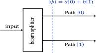
Figure 1. State preparation of a two-path interferometer in Greenberger–Yasin’s investigation of the wave-particle duality: the wave feature and particle feature with respect to the computational basis {∣0⟩, ∣1⟩} refer to those of the intermediate pure state ∣ψ⟩ generated by passing the input state through the first beam splitter [5]. |
2.2. Englert [6]
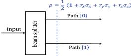
Figure 2. State preparation of a two-path interferometer in Englert’s investigation of the wave-particle duality: the wave feature and particle feature with respect to the computational basis {∣0⟩, ∣1⟩} refer to those of the intermediate mixed state ρ generated by passing the input state through the first beam splitter [6]. Though the setup is completely similar to that in figure 1, we depict it in this figure to emphasize that mixedness of the state yields significant difference for the wave-particle duality. |
2.3. Qian and Agarwal [34]
2.4. Dürr [7]
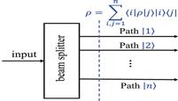
Figure 3. State preparation of an n-path interferometry in Dürr’s investigation of the wave-particle duality: the wave feature and particle feature with respect to the computational basis {∣i⟩: i = 1, 2, ⋯ , n} refer to that of the intermediate mixed state $\rho ={\sum }_{i,j=1}^{n}\langle i| \rho | j\rangle | i\rangle \langle j| $ generated by passing the input state through the first beam splitter [7]. |
3. Wave versus particle: quantitative aspects
| a | (a)${ \mathcal W }(\rho | {\rm{\Pi }})$ reaches its global minimum if the state ρ is classical (i.e. diagonal in the computational basis). |
| b | (b)${ \mathcal W }(\rho | {\rm{\Pi }})$ reaches its global maximum if ρ is pure and a uniform superposition of the states in the computational basis, i.e. ⟨i∣ρ∣i⟩ = 1/n for all i. |
| c | (c)${ \mathcal W }(\rho | {\rm{\Pi }})$ is invariant under permutations of the diagonal elements ⟨i∣ρ∣i⟩ of ρ. |
| d | (d)${ \mathcal W }(\rho | {\rm{\Pi }})$ is convex in ρ. |
| a | (a)${ \mathcal P }(\rho | {\rm{\Pi }})$ reaches its global maximum if ⟨i∣ρ∣i⟩ = 1 for some i. |
| b | (b)${ \mathcal P }(\rho | {\rm{\Pi }})$ reaches its global minimum if ⟨i∣ρ∣i⟩ = 1/n for all i. |
| c | (c)${ \mathcal P }(\rho | {\rm{\Pi }})$ is invariant under permutations of the diagonal elements ⟨i∣ρ∣i⟩ of ρ. |
| d | (d)${ \mathcal P }(\rho | {\rm{\Pi }})$ is convex in ρ. |
4. Wave-particle-mixedness triality
4.1. Quantifying wave feature via state uncertainty
| a | (a)${ \mathcal W }(\rho | {\rm{\Pi }})$ depends explicitly only on the off-diagonal elements of the density matrix of ρ in the computational basis {∣i⟩: i = 1, 2, …, n}, and is invariant under permutations of the off-diagonal elements. |
| b | (b)$0\leqslant { \mathcal W }(\rho | {\rm{\Pi }})\leqslant (n-1)/n$ for all quantum states. It is zero if and only if ρ is classical in the sense that its density matrix is diagonal in the computational basis, i.e., $\rho ={\sum }_{i=1}^{n}{p}_{i}| i\rangle \langle i| $ for some probabilities pi. While the maximal value (n − 1)/n is obtained if and only if the state is a maximal superposition of pure states in the computational basis, i.e., ρ = ∣φ⟩⟨φ∣ with $| \phi \rangle \,=\tfrac{1}{\sqrt{n}}{\sum }_{j=1}^{n}{{\rm{e}}}^{{\rm{i}}{\theta }_{j}}| j\rangle ,{\theta }_{j}\in {\mathbb{R}}.$ |
| c | (c)${ \mathcal W }(\rho | {\rm{\Pi }})$ is convex in ρ, that is, $\begin{eqnarray*}{ \mathcal W }\left(\sum _{i=1}^{k}{p}_{i}{\rho }_{i}| {\rm{\Pi }}\right)\leqslant \sum _{i=1}^{k}{p}_{i}{ \mathcal W }({\rho }_{i}| {\rm{\Pi }}),\end{eqnarray*}$ for a set of probabilities pi and quantum states ρi. |
4.2. Quantifying particle feature via measurement (un)certainty
| a | (a)${ \mathcal P }(\rho | {\rm{\Pi }})$ depends explicitly only on the diagonal elements of the density matrix of ρ in the computational basis {∣i⟩: i = 1, 2, …, n}, and is invariant under permutations of the diagonal elements. |
| b | (b)$1/n\leqslant { \mathcal P }(\rho | {\rm{\Pi }})\leqslant 1.$ The minimal value is obtained if ⟨i∣ρ∣i⟩ = 1/n for all i, while the maximal value is obtained if ⟨i∣ρ∣i⟩ = 1 for some i. |
| c | (c)${ \mathcal P }(\rho | {\rm{\Pi }})$ is convex in ρ. |
4.3. Quantifying mixedness via Brukner–Zeilinger invariant uncertainty
| a | (a)$0\leqslant { \mathcal M }(\rho )\leqslant (n-1)/n.$ The minimal value ${ \mathcal M }(\rho )=0$ is achieved if and only if ρ is a pure state, and the maximal value ${ \mathcal M }(\rho )=(n-1)/n$ is achieved if and only if ρ = 1/n is the maximally mixed state. |
| b | (b)${ \mathcal M }(\rho )$ is concave in ρ. |
Table 1. Various uncertainties. |
| Measurement uncertainty | ${ \mathcal U }(\rho | {\rm{\Pi }})=1-\displaystyle \sum _{i=1}^{n}\langle i| \rho | i{\rangle }^{2}$: Concave in ρ |
| Measurement certainty | ${ \mathcal P }(\rho | {\rm{\Pi }})=1-{ \mathcal U }(\rho | {\rm{\Pi }})=\displaystyle \sum _{i=1}^{n}\langle i| \rho | i{\rangle }^{2}$: Convex in ρ |
| State uncertainty | ${ \mathcal W }(\rho | {\rm{\Pi }})={\sum }_{i\ne j}| \langle i| \rho | j\rangle {| }^{2}$: Convex in ρ |
| Mixedness | ${ \mathcal M }(\rho )=1-\mathrm{tr}{\rho }^{2}$: Concave in ρ |
4.4. Wave-particle-mixedness triality
| a | (a)${ \mathcal W }(\rho | {\rm{\Pi }})$ summarizes the state uncertainty of ρ (in the von Neumann measurement Π induced by the paths), and can be regarded as a quantifier of interference potential. Large state uncertainty means large coherence, or equivalently, large potential for interference (fringe visibility). |
| b | (b)${ \mathcal P }(\rho | {\rm{\Pi }})$ quantifiers the measurement (un)certainty of Π induced by the paths (in the state ρ), and can be interpreted as a quantifier of path-detecting capability. Small measurement certainty (large uncertainty) means little information about the path. |
| c | (c)${ \mathcal M }(\rho )$ measures the uncertainty intrinsic to the state itself, as such, it can also be regarded as the capability of establishing correlations (entanglement) with other systems. |
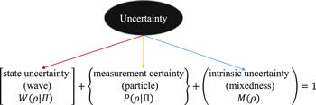
Figure 4. Wave-particle-mixedness triality as a resolution of unity: ${ \mathcal W }(\rho | {\rm{\Pi }})$ quantifies the uncertainty of state ρ in the paths described by Π and is interpreted as indicating the wave feature of the state, ${ \mathcal P }(\rho | {\rm{\Pi }})$ quantifies the measurement certainty of Π in the state ρ and is interpreted as indicating the particle feature of the state, ${ \mathcal M }(\rho )$ quantifies the intrinsic mixedness of the state ρ. These three kinds of uncertainties add up to unity. This constitutes our wave-particle-mixedness complementarity in a form of information conservation. |
| a | (a)When ρ = ∣ψ⟩⟨ψ∣ with $| \psi \rangle ={\sum }_{i=1}^{n}| i\rangle /\sqrt{n},$ one expects the maximal interference, the minimal path information, and the minimal mixedness. Indeed, ${ \mathcal W }(\rho | {\rm{\Pi }})=(n-1)/n$ (the maximal interference), ${ \mathcal P }(\rho | {\rm{\Pi }})=1/n$ (the minimal path information), ${ \mathcal M }(\rho )=0$ (the minimal mixedness), which is consistent with our expectation. |
| b | (b)When ρ = ∣i⟩⟨i∣ for some i, one expects the vanishing interference, the maximal path information, and the minimal mixedness. Indeed, ${ \mathcal W }(\rho | {\rm{\Pi }})=0$ (the vanishing interference), ${ \mathcal P }(\rho | {\rm{\Pi }})=1$ (the maximal path information), ${ \mathcal M }(\rho )=0$ (the minimal mixedness), which is consistent with our expectation. |
| c | (c)When ρ = 1/n, one expects the minimal interference, the minimal path information, and the maximal mixedness. Indeed, ${ \mathcal W }(\rho | {\rm{\Pi }})=0$ (the minimal interference), ${ \mathcal P }(\rho | {\rm{\Pi }})=1/n$ (the minimal path information), ${ \mathcal M }(\rho )=(n-1)/n$ (the maximal mixedness), which is also consistent with our expectation. |
Table 2. Some extreme cases for the triality relation ${ \mathcal W }(\rho | {\rm{\Pi }})+{ \mathcal P }(\rho | {\rm{\Pi }})+{ \mathcal M }(\rho )=1$. |
| ρ | ${ \mathcal W }(\rho | {\rm{\Pi }})$ | ${ \mathcal P }(\rho | {\rm{\Pi }})$ | ${ \mathcal M }(\rho )$ | Sum |
|---|---|---|---|---|
| $\tfrac{1}{n}{\sum }_{i,j=1}^{n}| i\rangle \langle j| $ | $\tfrac{n-1}{n}$ (max) | $\tfrac{1}{n}$ (min) | 0 (min) | 1 |
| ∣i⟩⟨i∣ | 0 (min) | 1 (max) | 0 (min) | 1 |
| $\tfrac{1}{n}1$ | 0 (min) | $\tfrac{1}{n}$ (min) | $\tfrac{n-1}{n}$ (max) | 1 |
5. Illustration and comparison
Table 3. Comparisons between our result, Englert’s duality, Qian–Agarwal’s duality, for a qubit state. Here ρ = (1 + rxσx + ryσy + rzσz)/2, Π = {∣0⟩⟨0∣, ∣1⟩⟨1∣}. |
| Englert | Qian and Agarwal | Our result | |
|---|---|---|---|
| Wave | ${V}_{{\rm{E}}}(\rho | {\rm{\Pi }})=\sqrt{{r}_{x}^{2}+{r}_{y}^{2}}$ | ${V}_{\mathrm{QA}}(\rho | {\rm{\Pi }})=\sqrt{{r}_{x}^{2}+{r}_{y}^{2}}$ | ${ \mathcal W }(\rho | {\rm{\Pi }})=({r}_{x}^{2}+{r}_{y}^{2})/2$ |
| Particle | PE(ρ∣Π) = ∣rz∣ | PQA(ρ∣Π) = ∣rz∣ | ${ \mathcal P }(\rho | {\rm{\Pi }})=(1+{r}_{z}^{2})/2$ |
| Purity/Mixedness | Not mentioned | ${\mu }_{S}(\rho )=\sqrt{{r}_{x}^{2}+{r}_{y}^{2}+{r}_{z}^{2}}$ | ${ \mathcal M }(\rho )=(1-({r}_{x}^{2}+{r}_{y}^{2}+{r}_{z}^{2}))/2$ |
| Duality/Triality | ${P}_{{\rm{E}}}^{2}(\rho | {\rm{\Pi }})+{V}_{{\rm{E}}}^{2}(\rho | {\rm{\Pi }})\leqslant 1$ | ${P}_{\mathrm{QA}}^{2}(\rho | {\rm{\Pi }})+{V}_{\mathrm{QA}}^{2}(\rho | {\rm{\Pi }})={\mu }_{S}^{2}(\rho )$ | ${ \mathcal P }(\rho | {\rm{\Pi }})+{ \mathcal W }(\rho | {\rm{\Pi }})+{ \mathcal M }(\rho )=1$ |
Table 4. Comparisons between our result, Dürr’s result and Jacob–Bergou’s result. Here Π = {∣i⟩⟨i∣: i = 1, 2, ⋯ , n}, ρij = ⟨i∣ρ∣j⟩. |
| Dürr | Jacob and Bergou | Our result | |
|---|---|---|---|
| Wave | ${V}_{{\rm{D}}}^{2}(\rho | {\rm{\Pi }})=\tfrac{n}{n-1}{\sum }_{i\ne j}| {\rho }_{{ij}}{| }^{2}$ | ${V}_{\mathrm{JB}}^{2}(\rho | {\rm{\Pi }})=2{\sum }_{i\ne j}| {\rho }_{{ij}}{| }^{2}$ | ${ \mathcal W }(\rho | {\rm{\Pi }})={\sum }_{i\ne j}| {\rho }_{{ij}}{| }^{2}$ |
| Particle | ${P}_{{\rm{D}}}^{2}(\rho | {\rm{\Pi }})=\tfrac{n}{n-1}{\sum }_{i\,=\,1}^{n}{\left({\rho }_{{ii}}-\tfrac{1}{n}\right)}^{2}$ | ${P}_{\mathrm{JB}}^{2}(\rho | {\rm{\Pi }})=2({\sum }_{i=1}^{n}{\rho }_{{ii}}^{2}-\tfrac{1}{n})$ | ${ \mathcal P }(\rho | {\rm{\Pi }})={\sum }_{i=1}^{n}{\rho }_{{ii}}^{2}$ |
| Mixedness | $\tfrac{n}{n-1}(1-\mathrm{tr}{\rho }^{2})$ | Not mentioned | ${ \mathcal M }(\rho )=1-\mathrm{tr}{\rho }^{2}$ |
| Triality | Equation ( | Equation ( | ${ \mathcal P }(\rho | {\rm{\Pi }})+{ \mathcal W }(\rho | {\rm{\Pi }})+{ \mathcal M }(\rho )=1$ |