


1. Introduction
Quantum optomechanics techniques now provide a new approach for mechanical resonators as novel systems for quantum science. During the 1990s, several aspects of quantum cavity optomechanical systems started to be explored theoretically [1]. It was also pointed out that for extremely strong optomechanical coupling the resulting quantum nonlinearities could give rise to nonclassical and entangled states of the light field and the mechanics [2].
Recently optomechanical systems have been used to study the quantum effects of macroscopic objects. A scheme to prepare a macroscopic mechanical oscillator in a cat-like state is proposed using state-of-the-art photonic crystal optomechanical system [3]. The investigation discussed in [4] shows that the use of squeezed states can significantly lengthen the lifetime of the cat states and improves the feasibility of generating cat states of large amplitude and with a greater degree of quantum macroscopic coherence. They show that the thermal decoherence of the dynamical cat states can be inhibited by a careful control of the squeezing of the reservoir. A feasible scheme in pulsed cavity optomechanics to generate the cat-like states of a macroscopic mechanical resonator is proposed by [5]. This approach can be used to produce non-Gaussian mechanical states, like optical-catalysis nonclassical states. Qin et al [6] proposed to create and stabilize long-lived macroscopic quantum superposition states in atomic ensembles, which opens up a new possibility towards the long-standing goal of generating large-size and long-lived cat states.
In the cavity quantum electrodynamics (QED), the interaction between a two-level atom and a quantum light field can be described by the quantum Rabi model (QRM). If the coupling strength between the atom and the field is quite weak, the Jaynes–Cummings model can be efficient. With the progress of the experimental techniques, the ultra-strong coupling strength regimes can be implemented in some solid-state devices such as superconducting circuits [7–11], quantum wells [12], cold atoms [13]. Recently, the QRM with arbitrary parameters has been realized in quantum simulations [14, 15], and the proposed scheme [14] shows that for ultra-strong coupling, a nonlinear coupling can also emerge, beside the linear dipole coupling between atom and field. This generalized model is called the quantum Rabi-Stark model (QRSM), for the nonlinear coupling term is associated with the dynamical Stark shift in the quantum optics.
QRSM has also attracted much attention in recent years [16–21]. Theoretically, the QRSM has been studied by the Bargmann space approach [16] and solved by the Bogoliubov operator approach [17]. Ref. [17] have given the G-function for the quantum Rabi-Stark model in a compact way, and declared that the regular spectrum can be determined by the zeros of the G-function.
In one of our previous works, we have proposed a scheme to prepare a macroscopically distinct mechanical superposition states of the mechanical oscillator using the QRM [22]. However, the distinguishable feature of the generated state is not strong. In this paper, we propose a new scheme to generate large-size cat states using the QRSM. The rest of this paper is organized as follows. In section 2 , we will introduce the physical model and its Hamiltonian. An effective Hamiltonian will be derived to depict the evolution of the system. In section 3 , we will study the preparation of the macroscopic quantum superposition state of the mechanical oscillator. Moreover, we will give a demonstration of the enhancement of the generated states by Wigner Function in section 4 . Finally, we will give some discussions in section 5 .
2. Model
Considering a cavity-QED system which consists of a two-level atom, single-mode Fabry–Perot cavity and a mechanical oscillator. There is a fixed mirror and a movable mirror in the cavity, the movable mirror coupled to the mechanical oscillator by opto-mechanical coupling. Resonance interaction occurs between spin and electromagnetic models restricted in the cavity. The Hamiltonian is given by ($\hslash =1$)
$\begin{eqnarray}H={H}_{{\rm{RS}}}+{H}_{{\rm{M}}}+{H}_{{\rm{RSM}}}.\end{eqnarray}$
Here, $\begin{eqnarray}{H}_{{\rm{RS}}}={H}_{{\rm{R}}}+{H}_{{\rm{Stark}}},\end{eqnarray}$
is the Rabi-Stark Hamiltonian.${H}_{{\rm{R}}}$ is the quantum Rabi Hamiltonian of the light–matter system written as
$\begin{eqnarray}{H}_{{\rm{R}}}=\omega {a}^{\dagger }a+\displaystyle \frac{\omega }{2}{\sigma }_{z}+{\rm{\Omega }}\left({\sigma }_{+}+{\sigma }_{-}\right)\left({a}^{\dagger }+a\right).\end{eqnarray}$
Here, ${a}^{\dagger }$($a$) represents the photonic creation (annihilation) operator of the single-mode cavity with frequency $\omega .$ {${\sigma }_{z},$ ${\sigma }_{\pm }$} are the Pauli matrices describing the two-level system which is supposed to be resonant with the cavity field. ω refers to the Rabi coupling of the atom and the cavity field, and for the ultrastrong coupling regime, we have η = ω/ω > 0.1.${H}_{{\rm{Stark}}}$ is the atom-cavity Stark interaction term with
$\begin{eqnarray}{H}_{{\rm{Stark}}}=\gamma {a}^{\dagger }a{\sigma }_{z}.\end{eqnarray}$
$\gamma {a}^{\dagger }a{\sigma }_{z}$ is the nonlinear coupling term added to the coupling of the atom-cavity [14, 15]. $\gamma $ is the non-linear Stark coupling strength. $\begin{eqnarray}{H}_{{\rm{M}}}={\omega }_{M}{b}^{\dagger }b,\end{eqnarray}$
is the Hamiltonian of the mechanical oscillator. ${b}^{\dagger }$($b$) is the creation (annihilation) operator of the mechanical oscillator separately, with the free frequency of the spring ${\omega }_{M}.$ And $\begin{eqnarray}{H}_{{\rm{RSM}}}={g}_{0}{a}^{\dagger }a\left(b+{b}^{\dagger }\right),\end{eqnarray}$
is the opto-mechanical interaction term. ${g}_{0}$ denotes the vacuum opto-mechanical coupling.For ${H}_{{\rm{R}}}$ in equation (3 ), a low-energy effective model was described [23]. And there are three energy eigen states with lowest energies, which were given by using quasi degenerate perturbation theory, at second order in $\eta .$ These eigenstates are:
$\begin{eqnarray}\begin{array}{l}\left|\left.G\right\rangle \right.=\left(1-\displaystyle \frac{{\eta }^{2}}{8}\right)\left|\left.0,g\right\rangle \right.+\displaystyle \frac{\eta }{2\sqrt{2}}\left(\left|\left.2-\right\rangle \right.-\left|\left.2+\right\rangle \right.\right)\\ \,+\displaystyle \frac{{\eta }^{2}}{4}\left(\left|\left.2-\right\rangle \right.+\left|\left.2+\right\rangle \right.\right),\end{array}\end{eqnarray}$
$\begin{eqnarray}\begin{array}{l}\left|\left.+\right\rangle \right.=\left(1-\displaystyle \frac{{\eta }^{2}}{8}-\displaystyle \frac{{\eta }^{2}}{32}\right)\left|1\left.+\right\rangle \right.-\displaystyle \frac{\eta }{4}\left(1+\displaystyle \frac{\eta }{2}\right)\left|1\left.-\right\rangle \right.\\ \,+\left(\displaystyle \frac{\eta }{2\sqrt{2}}+\displaystyle \frac{{\eta }^{2}}{2\sqrt{2}}\right)\left(\left|\left.3-\right\rangle \right.-\left|3\left.+\right\rangle \right.\right)\\ \,+\displaystyle \frac{\sqrt{3}{\eta }^{2}}{4\sqrt{2}}\left(\left|\left.3-\right\rangle \right.+\left|3\left.+\right\rangle \right.\right),\,\end{array}\end{eqnarray}$
$\begin{eqnarray}\begin{array}{l}\left|\left.-\right\rangle \right.=\left(1-\displaystyle \frac{{\eta }^{2}}{8}-\displaystyle \frac{{\eta }^{2}}{32}\right)\left|1\left.-\right\rangle \right.+\displaystyle \frac{\eta }{4}\left(1-\displaystyle \frac{\eta }{2}\right)\left|1\left.+\right\rangle \right.\\ \,+\left(\displaystyle \frac{\eta }{2\sqrt{2}}-\displaystyle \frac{{\eta }^{2}}{2\sqrt{2}}\right)\left(\left|\left.3-\right\rangle \right.-\left|3\left.+\right\rangle \right.\right)\\ \,+\displaystyle \frac{\sqrt{3}{\eta }^{2}}{4\sqrt{2}}\left(\left|\left.3-\right\rangle \right.+\left|3\left.+\right\rangle \right.\right),\end{array}\end{eqnarray}$
where $\{\left|\left.G\right\rangle \right.,\left|\left.\pm \right\rangle \right.\}$ are the three energy eigenstates of ${{\rm{H}}}_{{\rm{R}}}$ with lowest energies. $\left|\left.G\right\rangle \right.$ is the ground state with the energy of ${E}_{0}=-\omega /2-{\eta }^{2}\omega /2,$ and $\left|\left.\pm \right\rangle \right.$ are the excited states with the energies of ${E}_{\pm }=\omega /2\pm \eta \omega -{\eta }^{2}\omega /2.$ $\left|\left.g\right\rangle \right.$ and $\left|\left.e\right\rangle \right.$ are the atomic electronica ground state and excited state respectively. $\left|n\left.\pm \right\rangle =\left(\left|n,\left.g\right\rangle \right.\right.\right.\pm \left.\left|n-1,\left.e\right\rangle \right.\right)/\sqrt{2}$ ($n=1,2,3$) with $\left|\left.0\right\rangle \right.$ and $\left|\left.n\right\rangle \right.$ are Fock states of the cavity field.Since ${H}_{{\rm{RS}}}$ to be added by a term of ${H}_{{\rm{Stark}}}$ based on ${H}_{{\rm{R}}},$ we can revise the engen energies and eigen states once more, by using quasi degenerate perturbation theory, at second order in $\eta .$ Thus, we obtain the revised eigen energy as
$\begin{eqnarray}{E}_{0}=-\displaystyle \frac{\omega }{2}-\displaystyle \frac{{\eta }^{2}\omega }{2}-\displaystyle \frac{{\eta }^{2}}{4}\gamma ,\end{eqnarray}$
$\begin{eqnarray}{E}_{\pm }=\displaystyle \frac{\omega }{2}\pm \eta \omega -\displaystyle \frac{{\eta }^{2}\omega }{2}+\gamma \left(\displaystyle \frac{-1}{2}\pm \displaystyle \frac{\eta }{4}+\displaystyle \frac{3{\eta }^{2}}{4}\right).\end{eqnarray}$
And the revised ground state wave function and excited state wave function are respectively $\begin{eqnarray}\left|\left.G\right\rangle \right.=\left(1-\displaystyle \frac{{\eta }^{2}}{8}\right)\left|0,\left.g\right\rangle \right.-\displaystyle \frac{\eta }{2}\left|1,\left.e\right\rangle \right.+\displaystyle \frac{\sqrt{2}{\eta }^{2}}{4}\left|2,\left.g\right\rangle \right.,\end{eqnarray}$
$\begin{eqnarray}\begin{array}{l}\left|\left.\pm \right\rangle \right.=\displaystyle \frac{1}{\sqrt{2}}\left[\left(1\mp \displaystyle \frac{\eta }{4}-\displaystyle \frac{9{\eta }^{2}}{32}\right)+\displaystyle \frac{{\gamma }^{2}}{4{{\rm{\Omega }}}^{2}}\left(-\displaystyle \frac{1}{4}\pm \displaystyle \frac{3\eta }{8}\right.\right.\\ \,+\left.\left.\displaystyle \frac{25{\eta }^{2}}{32}\right)\right]\left|1,\left.g\right\rangle \right.\pm \displaystyle \frac{1}{\sqrt{2}}\left[\left(1\pm \displaystyle \frac{\eta }{4}-\displaystyle \frac{{\eta }^{2}}{32}\right)\right.\\ \left.\,-\displaystyle \frac{{\gamma }^{2}}{4{{\rm{\Omega }}}^{2}}\left(-\displaystyle \frac{1}{4}\pm \displaystyle \frac{3\eta }{8}+\displaystyle \frac{25{\eta }^{2}}{32}\right)\right]\left|0,\left.e\right\rangle \right.\\ \,-\left(\displaystyle \frac{\eta }{2}\pm \displaystyle \frac{{\eta }^{2}}{2}\right)\left|2,\left.e\right\rangle \right.+\displaystyle \frac{\sqrt{3}{\eta }^{2}}{4}\left|3,\left.g\right\rangle \right..\end{array}\end{eqnarray}$
According to the perturbation theory and equations (10 )–(13 ), we can get the valid range of the coupling strength $\gamma $ by satisfying the condition of $\left|\tfrac{\left\langle \left.+\right|\right.\gamma {a}^{\dagger }a{\sigma }_{z}\left|-\right\rangle }{{E}_{-}-{E}_{+}}\right|=\tfrac{\gamma /\omega \left(1-\displaystyle \tfrac{3{\eta }^{2}}{4}\right)}{4\eta }\ll 1.$ Here and in the following, we take $\omega =1.$ So we can get the valid range of the coupling strength $\gamma $ would be $\gamma \ll \tfrac{16\eta }{4-3{\eta }^{2}}\sim 4\eta .$ The obtained approximated eigen energies can also be compared with the regular energy spectra of QRSM given by [17]. For example, figure 1(a) shows the lowest three eigen energies for varying $\eta $ with $\gamma =0.25$ and $\eta =0.1,$ which are in good agreement with the lowest three eigen energies induced by the results in [17] (seeing figures 1(b) and (c)). Figure 1(b) shows the energy spectra of QRSM deduced from [17] for $\gamma =0.25.$ It can be seen that for $\eta \lt 0.3,$ the evolution of the lowest three eigen energies, are almost same to that in figure 1(a) deduced from our approximate model. Figure 1(c) plots the G-curves for $\gamma =0.25$ and $\eta =0.1$ based on the conclusions in [17]. The zeros in figure 1(c) can be easily detected, and then a good agreement can also be obtained. According to equations (10 ) and (11 ), for $\gamma =0.25,$ $\eta =0.1,$ we get ${E}_{+}\approx 0.48,{E}_{-}\approx 0.27,{E}_{0}\approx -0.51.$ From figures 1(c) or (b), we can get ${E}_{+}\approx 0.54,{E}_{-}\approx 0.21,{E}_{0}\approx -0.51$ for $\gamma =0.25,$ $\eta =0.1.$ Thus, our model is in good agreement with that in [17].
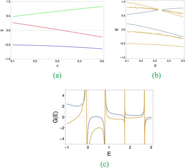
Figure 1. (a) The lowest three eigen energies of QRSM for $\gamma =0.25,$ $\eta =0.1.$ Green line and Red line are for ${E}_{+}$ and ${E}_{-}$ respectively. The Blue line is for ${E}_{0}.$ (b) Energy spectra deduced from [17] for $\gamma =0.25.$ The irregular broken lines are for the poles of the G-function. (c) G-curves for $\gamma =0.25,$ $\eta =0.1.$ |
Then by using this low-energy effective model, we can write the effective Hamilton of $H$ as
$\begin{eqnarray}\begin{array}{l}{H}^{{\rm{eff}}}={\omega }_{+}\left|+\right\rangle \left\langle \left.+\right|\right.+{\omega }_{-}\left|\left.-\right\rangle \right.\left\langle \left.-\right|\right.+{\omega }_{M}{b}^{\dagger }b+{g}_{0}\\ \,\times \left(b+{b}^{\dagger }\right)\left({\alpha }_{+}\left|+\right\rangle \left\langle \left.+\right|\right.+{\alpha }_{-}\left|+\right\rangle \left\langle \left.-\right|\right.+\xi \right).\end{array}\end{eqnarray}$
Here, we omitted terms proportional to the operators $\left|\pm \right\rangle \left\langle \left.\mp \right|\right.$ in a rotating-wave approximation [23], and $\xi =\tfrac{{\eta }^{2}}{4},$ $\begin{eqnarray}\begin{array}{l}{\alpha }_{\pm }=\displaystyle \frac{1}{2}\mp \displaystyle \frac{\eta }{4}+\displaystyle \frac{{\gamma }^{2}}{4{{\rm{\Omega }}}^{2}}\left(-\displaystyle \frac{1}{4}\pm \displaystyle \frac{7\eta }{16}+\displaystyle \frac{97{\eta }^{2}}{128}\right)\\ \,+\displaystyle \frac{{\gamma }^{4}}{32{{\rm{\Omega }}}^{4}}\left(\displaystyle \frac{1}{16}\pm \displaystyle \frac{3\eta }{16}-\displaystyle \frac{{\eta }^{2}}{4}\right),\end{array}\end{eqnarray}$
$\begin{eqnarray}\begin{array}{l}{\omega }_{\pm }=\omega \pm \eta \omega +\gamma \left(-1\pm \displaystyle \frac{\eta }{2}+\displaystyle \frac{7{\eta }^{2}}{4}\right)-\displaystyle \frac{{\gamma }^{3}}{4{{\rm{\Omega }}}^{2}}\\ \,\times \left(-\displaystyle \frac{1}{4}\pm \displaystyle \frac{7\eta }{16}+\displaystyle \frac{97{\eta }^{2}}{128}\right)-\displaystyle \frac{{\gamma }^{5}}{32{{\rm{\Omega }}}^{4}}\left(\displaystyle \frac{1}{16}\mp \displaystyle \frac{3\eta }{16}-\displaystyle \frac{{\eta }^{2}}{4}\right).\end{array}\end{eqnarray}$
We also assume that the opto-mechanical coupling is modulated by ${g}_{0}\to {g}_{0}\,\cos (vt),$ with cosine law regularly. $v={\omega }_{M}-\delta $ is the modulating frequency. $\delta $ is the detuning caused by modulation. In the interaction picture, the effective Hamiltonian can be given as
$\begin{eqnarray}{H}_{{\rm{I}}}^{{\rm{eff}}}=\displaystyle \frac{{g}_{0}}{2}\left(b{{\rm{e}}}^{-{\rm{i}}\delta t}+{b}^{\dagger }{{\rm{e}}}^{{\rm{i}}\delta t}\right)\left({\alpha }_{+}\left|\left.+\right\rangle \left.\left\langle +\right.\right|\right.+{\alpha }_{-}\left|\left.-\right\rangle \left.\left\langle -\right.\right|\right.+\xi \right).\end{eqnarray}$
3. Macroscopic quantum superposition state of the mechanical oscillator
At time $t=0,$ we assume that the initial state of the whole system to be $\left|\left.\pm \right\rangle \otimes {\left|0\right.}_{m}\right.,$ where ${\left.\left|0\right.\right\rangle }_{m}$ is the vacuum state of the mechanical oscillator. by applying the propagator associated with ${H}_{{\rm{I}}}^{{\rm{eff}}}$ on the initial state, the evolution state of the whole system at time $t$ in the interaction picture can be derived as
$\begin{eqnarray}{\left|{\rm{\Psi }}\left.\left(t\right)\right\rangle \right.}_{\pm }^{I}={{\rm{e}}}^{P+{\rm{i}}{Q}_{\pm }}\left|\left.\pm \right\rangle \right.\left|\left.{F}_{\pm }\right\rangle \right.,\end{eqnarray}$
with $\begin{eqnarray}P=-\displaystyle \frac{{{{\rm{g}}}_{0}}^{2}{\xi }^{2}}{2{\delta }^{2}}{\sin }^{2}\left(\displaystyle \frac{\delta t}{2}\right),\end{eqnarray}$
$\begin{eqnarray}{Q}_{\pm }=\displaystyle \frac{{{{\rm{g}}}_{0}}^{2}{\alpha }_{\pm }}{4\delta }\left(2\xi +{\alpha }_{\pm }\right)t-\displaystyle \frac{{{{\rm{g}}}_{0}}^{2}{\alpha }_{\pm }}{4{\delta }^{2}}\left(2{\rm{\xi }}+{\alpha }_{\pm }\right)\sin \left(\delta t\right),\end{eqnarray}$
$\begin{eqnarray}{F}_{\pm }=-\displaystyle \frac{{{\rm{g}}}_{0}}{2\delta }\left({{\rm{e}}}^{{\rm{i}}\delta t}-1\right)({\alpha }_{\pm }+\xi ).\end{eqnarray}$
$\left|\left.{F}_{\pm }\right\rangle \right.$ are the coherent states of the mechanical oscillator. Transforming ${\left|{\rm{\Psi }}\left.\left(t\right)\right\rangle \right.}_{\pm }^{I}$ into the Schrödinger picture, we can get the evolution state ${\left|{\rm{\Psi }}\left.\left(t\right)\right\rangle \right.}_{\pm }$ of the total system in the Schrödinger picture as
$\begin{eqnarray}{\left|{\rm{\Psi }}\left.\left(t\right)\right\rangle \right.}_{\pm }={{\rm{e}}}^{P+{\rm{i}}{v}_{\pm }(t)}\left|\left.\pm \right\rangle \right.\left|\left.{\beta }_{\pm }\right\rangle \right.,\end{eqnarray}$
with $\begin{eqnarray}{v}_{\pm }\left(t\right)=-\left[{\omega }_{\pm }-\displaystyle \frac{{{g}_{0}}^{2}{\alpha }_{\pm }}{4\delta }\left(2\xi +{\alpha }_{\pm }\right)\right]t-{\left(\displaystyle \frac{{g}_{0}{\alpha }_{\pm }}{2\delta }\right)}^{2}\,\sin \left(\delta t\right),\end{eqnarray}$
and $\begin{eqnarray}{\beta }_{\pm }\left(t\right)=-\displaystyle \frac{{\rm{i}}{g}_{0}({\alpha }_{\pm }+\xi )}{\delta }\,\sin \left(\displaystyle \frac{\delta t}{2}\right){{\rm{e}}}^{-{\rm{i}}\left({\omega }_{M}-\displaystyle \frac{\delta }{2}\right)t}.\end{eqnarray}$
Now we assume that for time $t=0,$ the initial state of the atom-cavity to be $\left|0,e\right.,$ and the mechanical oscillator to be in the state of ${\left.\left|0\right.\right\rangle }_{m},$ i.e., the initial state of the whole system is22 ), the evolution state of the whole system at time $t$ in the Schrödinger picture can be obtained as
$\begin{eqnarray}\left|{\rm{\Psi }}\left.\left(t=0\right)\right\rangle \right.=\left|0\left.e\right\rangle \right.\otimes {\left|\left.0\right\rangle \right.}_{m}=\displaystyle \frac{1}{\sqrt{2}}\left[\left|\left.+\right\rangle \right.\right.-\left|\left.\left.-\right\rangle \right]\otimes {\left.\left|0\right.\right\rangle }_{m}\right..\end{eqnarray}$
According to equation ( $\begin{eqnarray}\left|{\rm{\Psi }}\left.\left(t\right)\right\rangle \right.=\displaystyle \frac{1}{\sqrt{2}}\left[{{\rm{e}}}^{P+{\rm{i}}{v}_{+}\left(t\right)}\left.\left|+\right.\right\rangle \left|\left.{\beta }_{+}\right\rangle \right.-{{\rm{e}}}^{P+{\rm{i}}{v}_{-}\left(t\right)}\left|\left.-\right\rangle \right.\left|\left.{\beta }_{-}\right\rangle \right.\right].\end{eqnarray}$
Taking equation (13 ) into the equation (26 ), we can rewrite $\left|{\rm{\Psi }}\left(t\right)\right.$ as
$\begin{eqnarray}\begin{array}{l}\left|{\rm{\Psi }}\left.\left(t\right)\right\rangle \right.=\displaystyle \frac{1}{\sqrt{2}}\left[\left|1,\left.g\right\rangle \right.\left|{\left.{\varphi }_{1g}\right\rangle }_{m}\right.\right.+\left|0,\left.e\right\rangle \right.\left|{\left.{\varphi }_{0e}\right\rangle }_{m}\right.\\ \,+\left|2,\left.e\right\rangle \right.\left|{\left.{\varphi }_{2e}\right\rangle }_{m}\right.+\left.\left|3,\left.g\right\rangle \right.\left|{\left.{\varphi }_{3g}\right\rangle }_{m}\right.\right].\end{array}\end{eqnarray}$
Here, $\left|{\left.{\varphi }_{1g}\right\rangle }_{m}\right.,\left|{\left.{\varphi }_{0e}\right\rangle }_{m}\right.,\left|{\left.{\varphi }_{2e}\right\rangle }_{m}\right.$ and $\left|{\left.{\varphi }_{3g}\right\rangle }_{m}\right.$ are the evolution states of the mechanical oscillator at time $t,$ having the form of $\begin{eqnarray}\begin{array}{l}\left|{\left.{\varphi }_{1g}\right\rangle }_{m}\right.=\displaystyle \frac{1}{\sqrt{2}}{{\rm{e}}}^{P+{\rm{i}}{v}_{+}\left(t\right)}\left[\left(1-\displaystyle \frac{\eta }{4}-\displaystyle \frac{9{\eta }^{2}}{32}\right)\right.\\ \,+\left.\displaystyle \frac{{\gamma }^{2}}{4{{\rm{\Omega }}}^{2}}\left(-\displaystyle \frac{1}{4}+\displaystyle \frac{3\eta }{8}+\displaystyle \frac{25{\eta }^{2}}{32}\right)\right]\left|\left.{\beta }_{+}\right\rangle \right.\\ \,-\displaystyle \frac{1}{\sqrt{2}}{{\rm{e}}}^{P+{\rm{i}}{v}_{-}\left(t\right)}\left[\left(1+\displaystyle \frac{\eta }{4}-\displaystyle \frac{9{\eta }^{2}}{32}\right)\right.\\ \,+\left.\displaystyle \frac{{\gamma }^{2}}{4{{\rm{\Omega }}}^{2}}\left(-\displaystyle \frac{1}{4}-\displaystyle \frac{3\eta }{8}+\displaystyle \frac{25{\eta }^{2}}{32}\right)\right]\left|\left.{\beta }_{-}\right\rangle \right.,\end{array}\end{eqnarray}$
$\begin{eqnarray}\begin{array}{l}\left|{\left.{\varphi }_{0e}\right\rangle }_{m}\right.=\displaystyle \frac{1}{\sqrt{2}}{{\rm{e}}}^{P+{\rm{i}}{v}_{+}\left(t\right)}\left[\left(1+\displaystyle \frac{\eta }{4}-\displaystyle \frac{{\eta }^{2}}{32}\right)\right.\\ \,-\left.\displaystyle \frac{{\gamma }^{2}}{4{{\rm{\Omega }}}^{2}}\left(-\displaystyle \frac{1}{4}+\displaystyle \frac{3\eta }{8}+\displaystyle \frac{25{\eta }^{2}}{32}\right)\right]\left|\left.{\beta }_{+}\right\rangle \right.\\ \,+\displaystyle \frac{1}{\sqrt{2}}{{\rm{e}}}^{P+{\rm{i}}{v}_{-}\left(t\right)}\left[\left(1-\displaystyle \frac{\eta }{4}-\displaystyle \frac{{\eta }^{2}}{32}\right)\right.\\ \,-\left.\displaystyle \frac{{\gamma }^{2}}{4{{\rm{\Omega }}}^{2}}\left(-\displaystyle \frac{1}{4}-\displaystyle \frac{3\eta }{8}+\displaystyle \frac{25{\eta }^{2}}{32}\right)\right]\left|\left.{\beta }_{-}\right\rangle \right.,\end{array}\end{eqnarray}$
$\begin{eqnarray}\begin{array}{l}\left|{\left.{\varphi }_{2e}\right\rangle }_{m}\right.=-\left(\displaystyle \frac{\eta }{2}+\displaystyle \frac{{\eta }^{2}}{2}\right){{\rm{e}}}^{P+{\rm{i}}{v}_{+}\left(t\right)}\left|\left.{\beta }_{+}\right\rangle \right.-\left(\displaystyle \frac{\eta }{2}-\displaystyle \frac{{\eta }^{2}}{2}\right)\\ \,\times {{\rm{e}}}^{{P}_{-}+{\rm{i}}{v}_{-}\left(t\right)}\left|\left.{\beta }_{-}\right\rangle \right.,\end{array}\end{eqnarray}$
$\begin{eqnarray}\left|{\left.{\varphi }_{3g}\right\rangle }_{m}\right.=\displaystyle \frac{\sqrt{3}{\eta }^{2}}{4}{{\rm{e}}}^{P+{\rm{i}}{v}_{+}\left(t\right)}\left|\left.{\beta }_{+}\right\rangle \right.-\displaystyle \frac{\sqrt{3}{\eta }^{2}}{4}{{\rm{e}}}^{P+{\rm{i}}{v}_{-}\left(t\right)}\left|\left.{\beta }_{-}\right\rangle \right..\end{eqnarray}$
It can be seen that $\left|{\left.{\varphi }_{1g}\right\rangle }_{m}\right.,$ $\left|{\left.{\varphi }_{0e}\right\rangle }_{m}\right.,$ $\left|{\left.{\varphi }_{2e}\right\rangle }_{m}\right.$ and $\left|{\left.{\varphi }_{3g}\right\rangle }_{m}\right.$ are all quantum superposition of the coherent state $\left|\left.{\beta }_{\pm }\right\rangle \right.,$ respectively. If we take a measurement to the atom or the cavity field state, a mechanical superposition state would be generated.For a macroscopically distinct coherent state, the coherent amplitude should be $\left|{\beta }_{\pm }\right|\gt 1$ and $\left\langle {\beta }_{+}| {\beta }_{-}\right\rangle \ll 1.$ It can be seen from equation (24 ) that ${\left|{\beta }_{\pm }\right|}_{\max }=\left|\tfrac{{{\rm{g}}}_{0}({\alpha }_{\pm }+\xi )}{\delta }\right|$ for $\delta t=\left(2k+1\right)\pi $ ($k$ is nonnegative integer). If the amplitudes satisfy ${\left|{\beta }_{\pm }\right|}_{\max }\gt 1,$ we should take $\left|\delta /{{\rm{g}}}_{0}\right|\lt \left|{\alpha }_{\pm }+\xi \right|.$ For $\left\langle {\beta }_{+}| {\beta }_{-}\right\rangle ={{\rm{e}}}^{-{{{\rm{g}}}_{0}}^{2}{\left({\alpha }_{-}-{\alpha }_{+}\right)}^{2}\,\sin \,{\left(\displaystyle \frac{\delta {\rm{t}}}{2}\right)}^{2}/\,(2{\delta }^{2})\,},$ we get ${\left\langle {\beta }_{+}| {\beta }_{-}\right\rangle }_{{\rm{\min }}}={{\rm{e}}}^{-{{{\rm{g}}}_{0}}^{2}{\left({\alpha }_{-}-{\alpha }_{+}\right)}^{2}/\,(2{\delta }^{2})}$ when $\delta t=\left(2k+1\right)\pi $ ($k\in Z$). $\left|\left.{\beta }_{+}\right\rangle \right.$ and $\left|\left.{\beta }_{-}\right\rangle \right.$ will be orthogonal if $\left\langle {\beta }_{+}| {\beta }_{-}\right\rangle =0,$ i.e., the two states are maximally distinct. Thus $\left|\delta /{{\rm{g}}}_{0}\right|$ should satisfy $\left|\delta /{{\rm{g}}}_{0}\right|\lt \left|{\alpha }_{\pm }+\xi \right|$ and $\left|\delta /{{\rm{g}}}_{0}\right|\ll \tfrac{\left|{\alpha }_{-}-{\alpha }_{+}\right|}{\sqrt{2}}$ simultaneously, for a generated macroscopically distinct coherent state.
Since the values of $\left|{\alpha }_{\pm }+\xi \right|$ in ${\left|{\beta }_{\pm }\right|}_{{\rm{\max }}}$and $\tfrac{\left|{\alpha }_{-}-{\alpha }_{+}\right|}{\sqrt{2}}$in ${\left\langle {\beta }_{+}| {\beta }_{-}\right\rangle }_{{\rm{\min }}}$ have both connection with $\gamma ,$ the valid value of $\left|\delta /{{\rm{g}}}_{0}\right|$ is also limited by $\gamma .$ Thus, we can improve the distinguishability between the two macroscopic states of $\left.\left|{\beta }_{+}\right.\right\rangle $ and $\left.\left|{\beta }_{-}\right.\right\rangle $ by adjusting $\left|\delta /{{\rm{g}}}_{0}\right|$ and $\gamma .$ The smaller $\left|\delta /{{\rm{g}}}_{0}\right|$ is, the better the distinguishability is. The larger the difference between ${\alpha }_{+}$ and ${\alpha }_{-}$ is, the better the distinguishability is.
We provide a demonstration of the curves of $\left|{\alpha }_{\pm }+\xi \right|$ and $\tfrac{\left|{\alpha }_{-}-{\alpha }_{+}\right|}{\sqrt{2}}$varying with $\gamma $ in figure 2. According to figures 2(a) and (b), it can be seen that for $0\lt \gamma \lt 0.13,$ we can choose a valid regime about $\left|\delta /{{\rm{g}}}_{0}\right|\lt 0.01,$ and for $0.15\lt \gamma \lt 0.28,$ we can choose a valid regime about $\left|\delta /{{\rm{g}}}_{0}\right|\lt \mathrm{0.04.}$ Then the coherent amplitude should satisfy $\left|{\beta }_{\pm }\right|\gt 1$ and $\left\langle {\beta }_{+}| {\beta }_{-}\right\rangle \ll 1,$ and the generated macroscopical coherent state can be macroscopically distinguished.
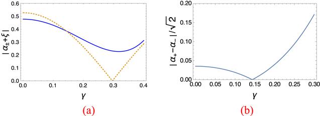
Figure 2. The demonstration of $\left|{\alpha }_{\pm }+\xi \right|$ and $\tfrac{\left|{\alpha }_{-}-{\alpha }_{+}\right|}{\sqrt{2}}$ varying with $\gamma $ (The dotted curve is for $\left|{\alpha }_{-}+\xi \right|$ and the solid curve is for $\left|{\alpha }_{+}+\xi \right|$). Here, we take $\eta =0.1,\tfrac{{\omega }_{M}}{{g}_{0}}=20.$ |
In figure 3, we give the demonstration of the evolution curves of $\left\langle {\beta }_{+}| {\beta }_{-}\right\rangle $ with $t$ for $\gamma =0$ (which corresponds to the circumstances using the Rabi model [22]) and $\gamma =0.25.$ It can be seen from the two curves that the minimum of $\left\langle {\beta }_{+}| {\beta }_{-}\right\rangle $ for $\gamma =0.25$ can get down to zero faster than the case for $\gamma =0,$ and sustaining zero for a much longer time, following which would improve the distinguishability of the macroscopically distinct coherent state in the Rabi-Stark model.
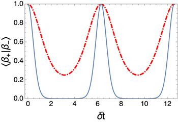
Figure 3. The demonstration of the evolution of $\left\langle {\beta }_{+}| {\beta }_{-}\right\rangle $ with time, for $\gamma =0$ (the dashing dotted curve) and $\gamma =0.25\,$(the solid curve). Here, we take $\delta =0.03{g}_{0},\eta =0.1,\tfrac{{\omega }_{M}}{{g}_{0}}=20.$ |
4. Wigner function
We can examine the macroscopic quantum coherence effects by the Wigner function. In this section, we take $\left|{\left.{\varphi }_{0e}\right\rangle }_{m}\right.$ as an example to demonstrate how strong macroscopic quantum coherence it has, by analyzing the properties of its Wigner function ${W}_{0e}\left(\alpha \right).$ Similar demonstrations can also be found for the other three states.
For the density matrix ρ, the Wigner function is defined by $W\left(\alpha \right)=\displaystyle \frac{2}{\pi }{\rm{Tr}}\left[{D}^{\dagger }(\alpha )\rho D(\alpha ){(-1)}^{{b}^{\dagger }b}\right],$ with $D(\alpha )$ is a displacement operator. So, we can get the Wigner function ${W}_{0e}\left(\alpha \right)$ of $\left|{\left.{\varphi }_{0e}\right\rangle }_{m}\right.$ by
$\begin{eqnarray}{W}_{0e}\left(\alpha \right)=\displaystyle \frac{2}{\pi }{\rm{Tr}}[{D}^{\dagger }(\alpha )\left|{\varphi }_{0e}\left.\left(t\right)\right\rangle \right.\left.\left\langle {\varphi }_{0e}\right.\left(t\right)\right|D(\alpha ){(-1)}^{{b}^{\dagger }b}].\end{eqnarray}$
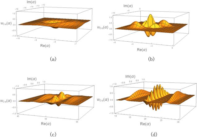
In figure 4, we give a demonstration of ${W}_{0e}\left(\alpha \right).$ Figures 4(a) and (b) are for $\gamma =0$ and $\gamma =0.25$ respectively with $\delta =0.03{g}_{0}.$ It can be seen that in figure 4(a), the two coherent states wave packets are so close that it is difficult to distinguish them, and their coherence is very weak. While in figure 4(b), there is a large distinct and well coherence between the two states wave packets.
Figure 4. The demonstration of the Wigner function ${{\rm{W}}}_{0e}\left(\alpha \right)$ at time $\delta t=\pi ,$ for (a) $\delta =0.03{g}_{0},$ $\gamma =0,$ (b) $\delta =0.03{g}_{0},$ $\gamma =0.25,$ (c) $\delta =0.01{g}_{0},\gamma =0,$ and (d) $\delta =0.01{g}_{0},$ $\gamma =0.25.$ Other parameters are $\eta =0.1,\tfrac{{\omega }_{M}}{{g}_{0}}=20.$ |
Also, figures 4(c) and (d) are for the demonstration of ${W}_{0e}\left(\alpha \right),$ with a smaller $\delta =0.01{g}_{0}$ respectively for $\gamma =0{\rm{and}}\,\gamma =0.25.$ It can be seen that in figure 4(c), the two coherent states have slightly more obvious distinguishability and slightly stronger coherence than figure 4(a). This is due to the reduction of ${\rm{\delta }}$ from $0.03{g}_{0}$ to $0.01{g}_{0}.$ While it can be seen that in figure 4(d), when $\gamma $ increases from 0 to 0.25, the distinguishability and the coherence between the two states will be significantly enhanced than figure 4(c).
5. Conclusion
In this article, we have proposed a method to further improve the preparation of macroscopically distinct quantum superposition state, by a Rabi-Stark coupling opto-mechanical system, compared with the scheme by a Rabi model. Firstly, in a low-energy subspace of the QRSM, we revised the eigen energies and eigen states of the QRM by using quasi degenerate perturbation theory, and then we got the effective Hamiltonian of the whole system.
Compared with the QRM, we have shown that the Stark coupling can induce larger energy level differences between the dressed states. This movement of the energy levels can induce stronger coupling between the atom-cavity subsystem and the quantum mechanical oscillator, which would further enhance the generated macroscopic quantum coherence states to have a stronger quantum coherence effect, and therefore better able to be distinguished.