


1. Introduction
2. Model RB: an example of constraint satisfaction problems
| • | Step 1. To construct a single constraint, we randomly select k ( ≥ 2) distinct variables out of the n variables, and then randomly select exactly pdnk (p is the constraint tightness) different incompatible assignments out of dnk possible ones as the set Qa to restrict the values of these k variables. |
| • | Step 2. We repeat the above step to obtain $m={rn}\mathrm{ln}n$ independent constraints and their corresponding sets Qa (a = 1, 2, ⋯ ,m). |
Let ${p}_{s}=1-{{\rm{e}}}^{-\tfrac{\alpha }{r}}$. If $\alpha \gt \tfrac{1}{k}$, $r\gt 0$ are two constants and $k{{\rm{e}}}^{-\tfrac{\alpha }{r}}\geqslant 1$, then
Let ${r}_{s}=-\tfrac{\alpha }{\mathrm{ln}(1-p)}$. If $\alpha \gt \tfrac{1}{k}$, $0\lt p\lt 1$ are two constants and $k\geqslant \tfrac{1}{1-p}$, then
3. Maximal residual belief propagation algorithm
3.1. Belief propagation algorithm
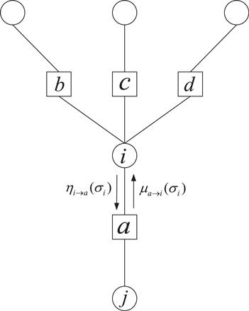
Figure 1. Part of a factor graph representing a random instance of binary model RB. Circles and squares denote the variable nodes and the constraint nodes, respectively. In the message passing algorithm of model RB, μa→i(σi) and ηi→a(σi) are the messages passed between a and i along the edge (a,i) in opposite directions. |
3.2. Maximal residual belief propagation algorithm
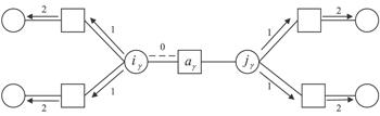
Figure 2. Local procedure of message updating based on maximal residuals on a factor graph. The edge (aγ, iγ) with the largest residual is selected for updating and then marked with 0, and the numbers 1 and 2 represent the order of message updating. |
| • | Type A: The variables that have been assigned with some values. |
| • | Type B: The variables not assigned with values, yet connected to the same constraints as the assigned ones. |
| • | Type C: Others. |
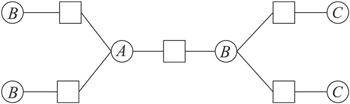
Figure 3. In the decimation process of the BPD algorithm, we classify the variables into three different types, indicated by A, B and C. |
| Input: A factor graph of a random instance generated by model RB, maximal iterations ${t}_{\max }$ used in the subroutines MRBP-UPDATE and MRBP-UPDATE*, and a precision parameter ϵ. |
| Output: A solution or ‘UNCONVERGED’. |
| Step 1 At T = 0: |
| 1.1 Run the subroutine MRBP-UPDATE. |
| 1.2 For each variable i, compute the marginal probability μi(σi) by equation ( |
| 1.3 Select the variable i* with the highest marginal probability from the n variables, and assign it to its most biased value ${\sigma }_{{i}^{* }}^{* }=\mathrm{argmax}{\mu }_{{i}^{* }}({\sigma }_{{i}^{* }})$. |
| Step 2 From T = 1 to n − 1: |
| 2.1 Run the subroutine MRBP-UPDATE*. |
| 2.2For each free (unfixed) variable i, compute the marginal probability μi(σi) by equation ( |
| 2.3 Select the variable i* with the highest marginal probability from the (n − T) free variables, and assign it to its most biased value ${\sigma }_{{i}^{* }}^{* }=\mathrm{argmax}{\mu }_{{i}^{* }}({\sigma }_{{i}^{* }})$. |
| 2.4 Check the energy function $E(\vec{\sigma })$ for the variables with assigned values according to equation ( |
| Step 3 If the assignment ${\vec{\sigma }}^{* }=({\sigma }_{1}^{* },{\sigma }_{2}^{* },\ldots ,{\sigma }_{n}^{* })$ of the n variables satisfies the m constraints simultaneously, output ${\vec{\sigma }}^{* }$ as a solution of the instance, otherwise output ‘UNCONVERGED’. |
| Step 1 At t = 0: for each edge (a, i), randomly initialize ${\mu }_{a\to i}^{0}({\sigma }_{i})\in [0,1]$. |
| Step 2 For the constraints from a = 1 to m: |
| 2.1 For each edge (a,i) with i ∈ V(a), use equation ( |
| 2.2 Use equation ( |
| Step 3 From t = 1 to ${t}_{\max }$: |
| 3.1 For each edge (a,i), calculate the residual ${\gamma }_{a\to i}^{t}$ using equation ( |
| 3.2 For i ∈ V(aγ), use equation ( |
| 3.3 For each edge (a,i), if $| {\mu }_{a\to i}^{t+1}({\sigma }_{i})-{\mu }_{a\to i}^{t}({\sigma }_{i})| \lt \varepsilon $ holds, break the loop and set ${\mu }_{a\to i}^{* }({\sigma }_{i})={\mu }_{a\to i}^{t}({\sigma }_{i})$. Otherwise go to 3.1 until all edges are marked. |
| 3.4 If $t={t}_{\max }$, output ‘UNCONVERGED’. |
| Step 1 At t = 0: |
| • For variables of Type A: skip; |
| • For variables of Type B: if the assignment of the variable i and the value of the fixed variable satisfy the corresponding constraint a, set ${\mu }_{a\to i}^{0}({\sigma }_{i})=1;$ otherwise, set ${\mu }_{a\to i}^{0}({\sigma }_{i})=0;$ |
| • For variables of Type C: uniformly initialize the values of ${\mu }_{a\to i}^{0}({\sigma }_{i})\in [0,1]$ at random. |
| Step 2 For the constraints from a = 1 to m: |
| 2.1 For each edge (a,i), where i ∈ V(a). |
| • For variables of Type A and Type B: skip; |
| • For variables of Type C: use equation ( |
| 2.2 Update ${\mu }_{a\to i}^{1}({\sigma }_{i})$. |
| • For variables of Type A: skip; |
| • For variables of Type B: let ${\mu }_{a\to i}^{1}({\sigma }_{i})={\mu }_{a\to i}^{0}({\sigma }_{i});$ |
| •For variables of Type C: use equation ( |
| Step 3 From t = 1 to ${t}_{\max }$: |
| 3.1 Compute the residual ${\gamma }_{a\to i}^{t}$. |
| • For variables of Type A and Type B: skip; |
| • For variables of Type C: for each edge (a,i), calculate the residual ${\gamma }_{a\to i}^{t}$ using equation ( |
| 3.2 For i ∈ V(aγ), use equation ( |
| 3.3 Determine whether the iterative equations converge or not. |
| • For variables of Type A and Type B: skip; |
| • For variables of Type C: for each edge (a,i), if $| {\mu }_{a\to i}^{t+1}({\sigma }_{i})-{\mu }_{a\to i}^{t}({\sigma }_{i})| \lt \varepsilon $ holds, break the loop and set ${\mu }_{a\to i}^{* }({\sigma }_{i})={\mu }_{a\to i}^{t}({\sigma }_{i})$. Otherwise go to 3.1 until all edges are marked. |
| 3.4 If $t={t}_{\max }$, output ‘UNCONVERGED’. |
4. Results
Table 1. For different problem sizes n, the domain size dn, the constraint number m, and the theoretical satisfiability threshold ps obtained by Theorem |
| n | α | r | dn | m | ps |
|---|---|---|---|---|---|
| 20 | 0.8 | 3 | 11 | 180 | ≃ 0.23 |
| 40 | 0.8 | 3 | 19 | 443 | ≃ 0.23 |
| 60 | 0.8 | 3 | 26 | 737 | ≃ 0.23 |
| 80 | 0.8 | 3 | 33 | 1052 | ≃ 0.23 |
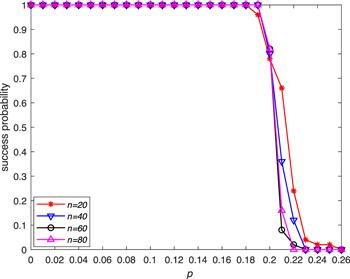
Figure 4. Fraction of satisfiable instances as a function of p obtained by the MRBP algorithm in solving 50 random instances generated by model RB. |
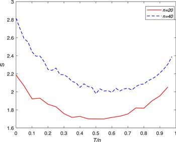
Figure 5. Entropy $S({x}_{i}^{T})$ of the decimated variables at each step T in the MRBP algorithm for binary model RB as a function of T/n at p = 0.1. |
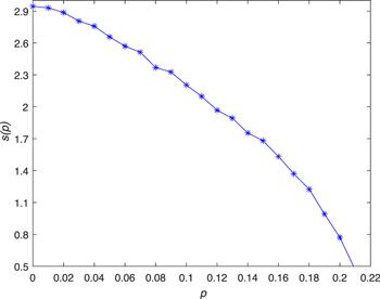
Figure 6. Mean degree of freedom s(p) on n variables in function of p during the execution of MRBP algorithm on a random instance generated by binary model RB for n = 40. |
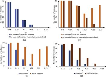
Figure 7. (a) Number of convergent instances and number of instances for which a solution can be found by algorithm 3 in [39] when solving 50 random instances of binary model RB for n = 40. (b) Results of the same content with (a) yet obtained from the MRBP algorithm. (c) and (d) Comparison of the two algorithms on the number of convergent instances and the number of successful instances, respectively. |
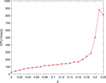
Figure 10. Running time of the MRBP algorithm as a function of p. We consider here n = 20. |