


1. Introduction
The last two decades have witnessed the rapid development of network science [1–3], with a growing number of scientific researchers from various fields plunging into the investigation of dynamics both of and on complex networks [4, 5]. The reason why complex networks have become the focus of scientific research is rooted in the fundamental understanding that many complex systems of interacting individuals can be described by networks [6, 7], in which nodes represent individuals and edges (i.e. links or connections) that join pairs of nodes mimic the interactions between the corresponding individuals.
It is well-known that one of the most important findings in the area of network science is that many complex networks in the real world exhibit a scale-free property [8–10] associated with a power-law degree distribution [11, 12], meaning that the probability P(k) for a randomly selected node to have k connections approximately follows a power law, P(k) ∝ k−γ, with the exponent γ varying for different empirical networks [13–18]. It is worth remarking that for many realistic networks the degree distribution is not a perfect power law but rather a right-skewed decay with an exponential cutoff [19, 20]. These observations suggest that the connectivity of nodes in real networks is extremely heterogeneous, which is in sharp contrast with the previous viewpoint by the random graph theory [21] that the nodes are homogeneous and their degrees obey a Poisson distribution where most degrees are close to the average degree. To provide a mechanism explanation for the universality of the power-law scaling behavior, Barabási and Albert proposed a growing network model [13, 22] with two indispensable ingredients—the growth and preferential attachment rules—where, at each time step, a node is added into the network with a certain number m of new links, each of which is connected to an old node with a probability proportional to the old node’s degree. They obtained a perfect scale-free network with the power-law exponent γ = 3 in the thermodynamic limit [22].
Since its publication, the pioneering work by Barabási and Albert [13] has swiftly sparked a surge of interest in the study of heterogeneous networks and a series of subsequent evolution models of growing networks have been studied [23–31]. Some variants of evolving network models are focused on the preferential attachment rule [23, 24, 26, 29–31]. For example, the fitness-based preferential attachment on the basis of ‘fit-get-richer’ principle [32, 33] has been considered as an alternative rule for attracting new links from newcomers to old nodes. Here, the fitness of a node is referred to as an intrinsic trait (or property) of the node [34], such as the innovation of a scientific paper or the personality of an individual. In comparison with the ‘rich-get-richer’ principle [33] (also known as the Matthew effect [35]) reflected by the degree-based preferential attachment in the Barabási–Albert model [13, 22], the fitness-based preferential attachment model of growing networks assume that the old nodes with large fitness values will have a larger probability to be attached by the newly added nodes, that is, the fitter the node is, the larger its degree will become [36].
In the literature, more general growing network models have also been proposed in terms of combining the degree- and fitness-based preferential attachment rules [33, 37]. For example, Bianconi and Barabási [38] considered the probability of node i to attract new links from new nodes is proportional to kiηi, where ki and ηi are the degree and fitness of node i, respectively. It was shown that the probability distribution of node fitness ρ(η) plays an important role in shaping the network structure [38]. Despite the success in characterizing the diversity of intrinsic property of individuals, introducing the fitness distribution into the preferential attachment network model has usually led to considerable difficulty in model analysis [37, 39, 40]. A simplifying approach for characterizing the intrinsic property of nodes is to introduce the so-called initial attractiveness in the preferential attachment network growth models, as done in [23, 37], where the initial attractiveness is assumed to be time-invariant and thus usually denoted by a constant parameter A. In these models, the probability for new nodes to connect an old one i is proportional to ki + A, the sum of the node i's degree ki and the initial attractiveness A.
Although very insightful, the above mentioned models for network growth have largely neglected the fact that during the growth of many real networks, aging of nodes occurs [19, 41–47]. For example, in scientific citation networks, old papers will gradually loose attractiveness since they are no longer sufficiently topical (or they are more often credited by intermediate citations) [43, 44]. In the movie actor networks [42], once popular stars are retiring from stage; while in the World Wide Web old famous web sites will loose favor to newly developed ones [48]. In view of these factors, it is of great importance to study the network evolving model that simultaneously account for the degree-dependent and initial attractiveness-based preferential attachment rules as well as the aging (or temporal) effects [45]. To this end, in this paper we propose a growing network model with a generalized preferential attachment rule that is based on degrees, initial attractiveness, and ages of nodes. We show that the resulting network has different structures depending on the initial attractiveness and aging parameters.
The paper is outlined as follows. In section 2 , we present our preferential attachment model for network growth with aging and initial attractiveness. In addition, the scaling behavior of the average degree and the degree distribution of the resulting network is analyzed. In section 3 , we present the numerical and simulation results with respect to different parameters. We conclude the paper in section 4 .
2. Preferential attachment network model with aging and initial attractiveness
In order to simultaneously take into account the degree- and initial attractiveness-based preferential linking as well as the aging effect, we propose a generalized preferential attachment model for the evolution of a growing network. Our model starts with a small number (m0) of nodes without any connections among them. Then, per unit time step, the network evolves as follows:
| i | (i)Growth—A new node is added. |
| ii | (ii)New links—The newly added node is preferentially attached to m (m ≤ m0) old nodes. |
| iii | (iii)Preferential attachment—The probability Πi for each old node i to be attached by the newly added node is proportional not only to the sum of the degree ki and the initial attractiveness Ai of node i but also to the power of its age, ${\tau }_{i}^{-\alpha }$, where α is the aging parameter and τi is node i's age. The choice of the power function ${\tau }_{i}^{-\alpha }$ to characterize the aging effect for old nodes is similar to the [41, 46, 47]. For simplicity, we assume an identical and constant initial attractiveness, A, for all nodes, i.e. Ai ≡ A. Thus, the preferential attachment probability to old node i is $\begin{eqnarray}{{\rm{\Pi }}}_{i}\propto ({k}_{i}+A){\tau }_{i}^{-\alpha }.\end{eqnarray}$ |
Suppose each node i is added into the network at time ti, then we can use the time tag ti to denote node i whose age τi(t) at an arbitrary time t (t ≥ ti) reads τi(t) = t − ti. Let k(ti, t) denote the average degree of node i at time t. Following the continuum approximation technique [13, 22], we obtain the following mean-field equation2 ) with respect to ti from 0 to t leads to
$\begin{eqnarray}\displaystyle \frac{\partial k({t}_{i},t)}{\partial t}=m\displaystyle \frac{\left[k({t}_{i},t)+A\right]{\left(t-{t}_{i}\right)}^{-\alpha }}{{\int }_{0}^{t}\left[k({t}_{j},t)+A\right]{\left(t-{t}_{j}\right)}^{-\alpha }{\rm{d}}{t}_{j}},\end{eqnarray}$
with the boundary condition k(t, t) = m, which holds since every newly added node has m links to old nodes. Integrating both sides of equation ( $\begin{eqnarray}{\int }_{0}^{t}\displaystyle \frac{\partial k({t}_{i},t)}{\partial t}{\rm{d}}{t}_{i}=m.\end{eqnarray}$
Note that $\begin{eqnarray}\displaystyle \frac{\partial }{\partial t}{\int }_{0}^{t}k({t}_{i},t){\rm{d}}{t}_{i}=k(t,t)+{\int }_{0}^{t}\displaystyle \frac{\partial k({t}_{i},t)}{\partial t}{\rm{d}}{t}_{i}=2m,\end{eqnarray}$
one immediately has the equality $\begin{eqnarray}{\int }_{0}^{t}k({t}_{i},t){\rm{d}}{t}_{i}=2{mt},\end{eqnarray}$
which means the total degree of all nodes is twice the number of links in the network.The homogeneous form of equation (2 ) suggests that we can seek a self-similar solution as a function of the single variable ti/t rather than two separate variables5 ) and (6 ) gives rise to2 ), we obtain8 ), we get9 ) can be taken as10 ) into equation (9 ) leads to13 ), we can derive the degree distribution P(k) of the network in a similar way to [22]. To do this, suppose $k({t}_{i},t)=C(t){t}_{i}^{-\beta }$ where C(t) = Ctβ with some constant C. Consequently, the probability for a node to have a degree equal to or smaller than k is14 ) is determined by the probability density function f(ti) of the random variable ti. To obtain the expression of f(ti), we make the following assumption. Note that in our model each node is added per unit time step and there are m0 + t nodes at time t (including m0 nodes at the initial step). Assume that we add each node at equal time intervals to the network. In the continuous time limit, this is equivalent to assuming that the entrance time ti is a random variable uniformly distributed in the time window [0, m0 + t]. In fact this trick was originally made in the classic Barabási–Albert scale-free network model (see the statement for equation (8) in [22]). Therefore, under the continuous limit the probability density of ti can be approximated as15 ) into equation (14 ) we have12 ) into (8 ):7 ) and (8 ) that
$\begin{eqnarray}k({t}_{i},t)=\kappa (x),\qquad x\equiv {t}_{i}/t.\end{eqnarray}$
Combining equations ( $\begin{eqnarray}{\int }_{0}^{1}\kappa (x){\rm{d}}x=2m.\end{eqnarray}$
Performing the variable transformation on equation ( $\begin{eqnarray}-x{\left(1-x\right)}^{\alpha }\displaystyle \frac{\mathrm{dln}[\kappa (x)+A]}{{\rm{d}}x}=\displaystyle \frac{m}{{\int }_{0}^{1}\tfrac{\kappa (x)+A}{{\left(1-x\right)}^{\alpha }}{\rm{d}}x}\equiv \beta ,\end{eqnarray}$
with κ(1) = m. Here, β is a constant to be determined. Solving equation ( $\begin{eqnarray}\mathrm{ln}\displaystyle \frac{\kappa (x)+A}{m+A}={\int }_{x}^{1}\displaystyle \frac{\beta }{y{\left(1-y\right)}^{\alpha }}{\rm{d}}y.\end{eqnarray}$
For α < 1 the integration on the right hand side of equation ( $\begin{eqnarray}\begin{array}{rcl}{\displaystyle \int }_{x}^{1}\displaystyle \frac{\beta }{y{\left(1-y\right)}^{\alpha }}{\rm{d}}y & = & -\beta \alpha x{\,}_{3}{F}_{2}(1,1,1+\alpha ;2,2;x)\\ & & -\beta \left[H(-\alpha )+\mathrm{ln}x\right],\end{array}\end{eqnarray}$
where 3F2( , , ; , ; ) is the hypergeometric function [49] and H( · ) is the harmonic number which can be derived as $\begin{eqnarray}H(x)=\psi (1+x)+{\gamma }_{{\rm{E}}},\end{eqnarray}$
with $\psi (x)=\tfrac{{\rm{d}}}{{\rm{d}}x}\mathrm{ln}\left({\rm{\Gamma }}(x)\right)=\tfrac{{\rm{\Gamma }}^{\prime} (x)}{{\rm{\Gamma }}(x)}$ being the digamma function and γE = 0.57721... the Euler-Mascheroni constant. Inserting equation ( $\begin{eqnarray}\begin{array}{rcl}\kappa (x)+A & = & (m+A){{\rm{e}}}^{-\beta \alpha x{\,}_{3}{F}_{2}(\mathrm{1,1,1}+\alpha ;\mathrm{2,2};x)}\\ & & \times {{\rm{e}}}^{-\beta [\psi (1-\alpha )+{\gamma }_{{\rm{E}}}]}{x}^{-\beta }.\end{array}\end{eqnarray}$
For x → 0, we have κ(x) ∝ x−β, that is, the constant β is the exponent of the average degree such that for ti ≪ t $\begin{eqnarray}k({t}_{i},t)\propto {\left({t}_{i}/t\right)}^{-\beta }.\end{eqnarray}$
This result implies that the average degree of old nodes exhibits a power-law scaling behavior with exponent β. Moreover, according to such scaling behavior of the average degree given by equation ( $\begin{eqnarray}P\left(k({t}_{i},t)\leqslant k\right)=P\left({t}_{i}\geqslant {\left[\displaystyle \frac{C(t)}{k}\right]}^{1/\beta }\right).\end{eqnarray}$
The probability on the right side of equation ( $\begin{eqnarray}f({t}_{i})=\displaystyle \frac{1}{{m}_{0}+t}.\end{eqnarray}$
Plugging equation ( $\begin{eqnarray}P\left(k({t}_{i},t)\leqslant k\right)=1-\displaystyle \frac{{\left[C(t)\right]}^{1/\beta }}{{m}_{0}+t}{k}^{-1/\beta }.\end{eqnarray}$
The probability density for P(k) can be obtained by $\begin{eqnarray}P(k)=\displaystyle \frac{\partial P\left(k({t}_{i},t)\leqslant k\right)}{\partial k}=\displaystyle \frac{{C}^{1/\beta }t}{\beta ({m}_{0}+t)}{k}^{-(1+1/\beta )}.\end{eqnarray}$
As a result, as t → ∞ , the degree distribution of the network has a power-law scaling for large k (small ti): $\begin{eqnarray}P(k)\propto {k}^{-\gamma },\quad \gamma \equiv 1+1/\beta .\end{eqnarray}$
Obviously, the calculation of the value of the exponent β is very important as it shapes the scaling behavior for both the average degree and the degree distribution. For this purpose, we obtain the following transcendental equation for β by substituting equations ( $\begin{eqnarray}\begin{array}{rcl}{\beta }^{-1} & = & \left(1+\displaystyle \frac{A}{m}\right){{\rm{e}}}^{-\beta \left[\psi (1-\alpha )+{\gamma }_{{\rm{E}}}\right]}\\ & & \times {\displaystyle \int }_{0}^{1}\displaystyle \frac{{{\rm{e}}}^{-\beta \alpha x{\,}_{3}{F}_{2}(\mathrm{1,1,1}+\alpha ;\mathrm{2,2};x)}}{{\left(1-x\right)}^{\alpha }{x}^{\beta }}{\rm{d}}x.\end{array}\end{eqnarray}$
In the special case of α = 0 when the aging effect is removed, it follows from equations ( $\begin{eqnarray}\beta =\displaystyle \frac{1}{2+A/m},\end{eqnarray}$
and hence $\begin{eqnarray}\gamma =3+A/m.\end{eqnarray}$
Furthermore, when the initial attractiveness is set to zero, A = 0, we have β = 1/2 and γ = 3, which recovers the result of the Barabási–Albert model [13, 22].In the more general case when α ≠ 0, it is hard to derive an analytic solution for β in the transcendental equation (8 ). In fact, according to equation (10 ), the solution for β pertaining to equation (19 ) exists only in the range − ∞ < α < 1. Note that although only the case of α ≥ 0 seems to be of realistic significance, we also consider the case of α < 0 since it does not cause any contradiction.
3. Simulations
In order to verify our theoretical analysis, we perform extensive stochastic simulations on our network model for different parameter values.
In figure 1 we present the results of the average connectivity k(ti, t) of node i versus its adding time ti at time t = 104. All the results are obtained by averaging over 200 independent realizations of Monte Carlo stochastic simulation. The observed linearity plotted in the log–log scale in all the panels (a), (b) and (c) of figure 1 indicates that there is a power-law scaling behavior $k({t}_{i},t)\propto {t}_{i}^{-\beta }$ for 1 ≤ ti ≤ 103, supporting the theoretical prediction by equation (13 ). Specifically, as shown in figure 1(a) for A = m = 4, in case of negative values of the aging parameter, i.e. α = −3, −2, −1, the average degree k(ti, t) decays very quickly (with a rather steep slope). On the other hand, when the aging parameter α rises from zero to 0.3, and to 0.7, the average degree k(ti, t) decays more and more slowly with a relatively smaller exponent β (this can also be clarified in figure 2). Interestingly, when the value of α becomes large enough, as shown in figure 1(a) for α = 3, the average degree of node i tends to be a constant k ≃ 8 (with the power-law exponent β ≃ 0) irrespective of its age τi (i.e. independent of the entering time ti of node i). In this situation, the decaying effect dominates the preferential linking such that each new node is only connected to the latest added m nodes. Therefore, each node has on average a number k = 2m of connections, half of which are connected to its latest m predecessors and the other half are connected by its m subsequent newcomers. In figure 1(b) we show the power-law decaying behavior of the average degree k(ti, t) versus ti for various values of A = 0, 4, 8, 12 with m = 4 and α = 0.3. As the value of A rises (equivalently, as the value of A/m rises), the power law decays more and more slowly. That is, the larger the value of A/m, the smaller value of the power exponent β (this can also be shown in figure 2). Moreover, as illustrated in figure 1(c), when we set A = m and change their values from 2 to 4, and to 6, three parallel power-law curves are observed in the log–log scale, suggesting the power exponent β is strongly dependent on the ratio A/m, which is consistent to the theoretical analysis given in equation (19 ).

Figure 1. The average degree k(ti, t) of node i at time t = 104 as a function of node i's entering time ti for (a) different values of α with A = m = 4 (from top to bottom, α = −3, −2, −1, 0, 0.3, 0.7, 3); (b) different values of A with m = 4 and α = 0.3 (from top to bottom, A = 0, 4, 8, 12); and (c) different values of m with A = m and α = 0.7 (from top to bottom, A = m = 2, 4, 6). |

Figure 2. Dependence of the exponent β of the power law scaling for the average degree $k({t}_{i},t)\propto {t}_{i}^{-\beta }$ on the aging parameter α and the ratio A/m. The lines are numerical solution of β obtained from equation ( |
In figure 2 we provide a full diagram for the dependence of the power exponent β on the aging parameter α and the ratio A/m. The lines in the plot represent the theoretical results of β calculated by numerical integration from equation (19 ) and the symbols with error bars correspond to the average results with standard deviation obtained from stochastic simulations. There is good agreement between theory and simulation. For a fixed value of the ratio A/m, as shown in each line, the power exponent β declines with α. In particular, as the aging decaying effect becomes strong (large α), the old node will loose the opportunity to accumulate connections. As a result, the larger the value of α, the smaller degree for old nodes (with small ti). More interestingly, as the value of α approaches 1, all lines converges at the limit β → 0. On the other hand, for a given α < 1, the value of β decreases with the increase of the value of the ratio A/m.
To exhibit a clearer scaling behavior for their relationship, in figure 3 we redraw the results in terms of 1/β as a function of the ratio A/m. The straight lines suggest that the reciprocal of the exponent β is a linear function of the ratio A/m, i.e. $\tfrac{1}{\beta }={C}_{1}\tfrac{A}{m}+{C}_{2}$, where C1 and C2 are coefficients that depend on α. In the special case α = 0, we have C1 = 1 and C2 = 2 according to equation (20 ).

Figure 3. The reciprocal of the exponent β of the power law scaling for the average degree $k({t}_{i},t)\propto {t}_{i}^{-\beta }$ as a function of the ratio A/m for various values of the aging parameter α. From bottom to top, the value of α is set to −2, −1, −0.5, 0, 2, 4, 6, 7 and 8. |
In figure 4 we present the simulation results of the degree distribution of the resulting network of size N = 106 for different parameter settings. As shown in figure 4(a), in the special case of α = 0 and A = 0, the degree distribution obtained from simulation (marked by black squares) follows a perfect power law, that is, we obtain a typical scale-free network. In this case, there is no aging effect and initial attractiveness, therefore our model is reduced to the classic Barabási–Albert scale-free network model [13, 22], in which the theoretical result of the degree distribution takes the form P(k) = 2m2k−3 (see the green line). It is clear that the simulation result agrees well with the theoretical outcome. In figure 4(b) we show that in the case when the aging effect is removed α = 0 and the initial attractiveness is included A = 4, the degree distribution has a power-law scaling behavior P(k) ∝ k−γ for large degree k. Direct comparison between the slope in the range k > 30 and the (pink dotted) guiding line suggests that the simulation result of the scaling exponent is in good agreement with the theoretical prediction γ = 5 by equation (21 ). In figure 4(c) we depict the the simulation results of degree distribution in the more general case when both aging effect and initial attractiveness are considered. The results show that when α < 1 the degree distribution scales as a power law for large k. In particular, as the value of the aging parameter α rises, the degree distribution becomes narrower and the exponent γ increases correspondingly (also see figure 5). On the other hand, when α is relatively large, the model will generate exponential networks. The log-linear plot in the inset of figure 4(c) shows that, for α = 1, 3, 5, the degree distribution of the network decays exponentially when k is greater than the average degree ⟨k⟩ = 2m = 4.

Figure 4. Degree distribution of the resulting network when the network size is N = 106 for different parameters. Panel (a) represents the special case when α = 0, A = 0, and m = 2, where black squares are simulation results and the green line stands for the theoretical result P(k) = 2m2k−3 obtained in the Barabási–Albert model [13, 22]. Panel (b) corresponds to the case when α = 0, A = 4, and m = 2. Panel (c) displays the degree distribution for different values of the aging parameter α when A = 4 and m = 2. |
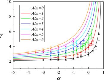
Figure 5. The scaling exponent γ of power-law degree distribution P(k) ∝ k−γ in the limit of large k as a function of the aging parameter α for various values of the ratio A/m. From bottom to top, the value of A/m is set to 0, 1, 2, 3, 4, 5 and 6. Lines are numerical solution obtained from equations ( |
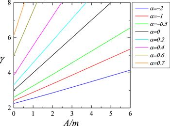
In figure 5 we plot the scaling exponent γ of the degree distribution P(k) ∝ k−γ for large k versus the aging parameter α for different values of A/m. Given the ratio A/m, the exponent γ increases with the aging parameter α. In particular, in the limit α → 1, the exponent γ becomes extremely large, meaning the network turns to be an exponential rather than a power-law network. This is in consistency with the simulation results given in figure 4(c). In addition, for any given α < 1, the exponent γ increases with the ratio A/m. Moreover, we demonstrate in figure 6 that the scaling exponent γ is linearly dependent on the ratio A/m. In fact, as illustrated in figure 3, the reciprocal of exponent β is linearly correlated with A/m, i.e. $1/\beta ={C}_{1}\tfrac{A}{m}+{C}_{2}$. Then the relationship γ = 1 + 1/β by equation (18 ) indicates that the exponent γ is also a linear function of the ratio A/m, namely, $\gamma ={C}_{1}\tfrac{A}{m}+({C}_{2}+1)$, which takes the form γ = 3 + A/m [equation (21 )] for α = 0. If we further assume A = 0, then we reproduce the scaling exponent γ = 3 discovered in the Barabási–Albert scale-free network model [13, 22].
Figure 6. The scaling exponent γ of power-law degree distribution P(k) ∝ k−γ in the limit of large k as a function of the ratio A/m for various values of the aging parameter α. From bottom to top, the value of α is set to −2, −1, −0.5, 0, 0.2, 0.4, 0.6 and 0.7. |
4. Conclusion
In this paper, we have studied a generalized growing model that integrates the aging effects into the preferential linking mechanism. In our model, the probability for newly added nodes to attach to an old node is not only proportional to the sum, k + A, of the degree k and initial attractiveness A of the old node but also proportional to an aging factor that is defined as a decaying function in terms of the age of the old node with an aging parameter, α. This preferential attachment rule is defined to account for the fact that the higher connectivity, the larger initial attractiveness, and the smaller age a node has, the higher probability for it to be attached to. Through continuous approximation and mean-field analysis, we have uncovered the scaling behavior for both the average connectivity and the degree distribution of the resulting network. The results from both theory and simulations have shown that for the region α < 1, the average connectivity k(ti, t) of a node i (that is added into the network at time ti) at the current time t scales as a power law $k({t}_{i},t)\propto {t}_{i}^{-\beta }$, especially when ti ≪ t. In addition, in the limit of large degree k, the degree distribution also scales as a power law P(k) ∝ k−γ with the scaling exponent γ = 1 + 1/β. More interestingly, we have found that the scaling exponents β and γ are both a linear function of the ratio, A/m, of the initial attractiveness A to the number m of emanating links from each new node.
It is worth mentioning that in the same direction as the present work, Sun et al [50] have recently developed a more generalized preferential attachment network model with degree, fitness and aging. In their model, the general fitness distribution (rather than initial attractiveness) is included to account for the ‘fit-get-richer’ principle. Their work focused on the time-invariant degree growth of network nodes; in contrast, the focus of our work is to uncover the scaling behavior of the average degree and the degree distribution when the network growth is subject to preferential attachment with initial attractiveness and aging effect.