How to accurately probe chemically reactive flows with essential thermodynamic nonequilibrium effects is an open issue. Via the Chapman–Enskog analysis, the local nonequilibrium particle velocity distribution function is derived from the gas kinetic theory. It is demonstrated theoretically and numerically that the distribution function depends on the physical quantities and derivatives, and is independent of the chemical reactions directly as the chemical time scale is longer than the molecular relaxation time. Based on the simulation results of the discrete Boltzmann model, the departure between equilibrium and nonequilibrium distribution functions is obtained and analyzed around the detonation wave. In addition, it has been verified for the first time that the kinetic moments calculated by summations of the discrete distribution functions are close to those calculated by integrals of their original forms.
Xianli Su, Chuandong Lin. Nonequilibrium effects of reactive flow based on gas kinetic theory[J]. Communications in Theoretical Physics, 2022, 74(3): 035604. DOI: 10.1088/1572-9494/ac53a0
1. Introduction
Chemical reactive flow is a complex physicochemical phenomenon which is ubiquitous in aerospace, energy and power fields, etc [1, 2]. It exhibits multiscale characteristics in temporal and spatial scales, incorporates various hydrodynamic and thermodynamic nonequilibrium effects [3]. The nonequilibrium effects exert significant influences on fluid systems especially in extremely complex environments [3], such as the spacecraft reentry into the atmosphere [4], multi-component reactive flow in porous media [5, 6], fuel cells [7, 8], phase separation [9], hydrodynamic instability [10], and detonation [11, 12]. At present, how to accurately probe, predict and analyze chemical reactive flows with essential nonequilibrium effects is still an open issue.
Actually, there are various classes of methodologies to retain the information of velocity distribution functions for fluid systems. For example, on the basis of the distribution function, Nagnibeda et al established the kinetic theory of transport processes and discussed the features of complex system strongly deviating from the thermal and chemical equilibrium [3]. Besides, on the microscopic level, the distribution function can be obtained by using the direct simulation Monte Carlo [13, 14], or molecular dynamics [15, 16]. As a kinetic mesoscopic methodology, the discrete Boltzmann method (DBM) is a special discretization of the Boltzmann equation in particle velocity space, and has been successfully developed to recover and probe the velocity distribution functions of nonequilibrium physical systems [11, 17–20].
In fact, the DBM is based on statistical physics and regarded as a variant of the traditional lattice Boltzmann method (LBM) [21–24]. Compared to standard LBMs, the DBM can address more issues, in particular to simulate the compressible fluid systems with significant nonequilibrium effects [17, 20, 25–30]. At present, there are two means to recover the velocity distribution functions. One relies on the analysis of the detailed nonequilibrium physical quantities to obtain the main features of the velocity distribution function in a qualitative way [11, 17, 18]. The other is to recover the detailed velocity distribution function by means of macroscopic quantities and their spatio derivatives quantitatively, which can be derived by using the Chapman–Enskog expansion [19, 20]. The two methods are consistent with each other [20].
In the rest of this paper, we firstly derive the nonequilibrium velocity distribution function of reactive fluid based on the Boltzmann equation in section 2. In section 3, we give a brief introduction of the DBM for compressible reactive flows. In section 4, we verify the consistency of theoretical and numerical results of the equilibrium or nonequilibrium manifestations of reactive flows. The nonequilibrium and equilibrium distribution functions as well as their differences are obtained and analyzed in section 5. Finally, section 6 concludes.
2. Derivation of velocity distribution function of reactive fluid
Now, let us introduce the popular Bhatanger–Gross–Krook (BGK) Boltzmann equation
where D = 2 denotes the dimensional translational degree of freedom, I stands for extra degrees of freedom due to vibration and/or rotation, and η represents the corresponding vibrational and/or rotational energies. Here n is the particle number density, u the hydrodynamic velocity, T the temperature, m = 1 the particle mass, and ρ = nm the mass density.
On the right-hand side of equation (1), R is the chemical term describing the change rate of the distribution function due to chemical reactions, i.e.
To derive the explicit expression of the chemical term, the following qualifications are assumed [26]: tmr < tcr < tsys, where tmr, tcr and tsys represent the time scale of molecular relaxation, the time scale of chemical reaction and the characteristic time scale of the system, respectively. Under the condition tmr < tcr, equation (3) can be approximated by
as f eq is the function of ρ, u, and T, respectively. Furthermore, the assumption tcr < tsys leads to the following conclusion: the chemical reaction results in the change of temperature directly, as the density and flow velocity remain unchanged during the rapid reaction process. Consequently, equation (4) can be reduced to
where Q indicates the chemical heat release per unit mass of fuel, $\lambda ^{\prime} $ is the change rate of the mass fraction of chemical product. Additionally, a two-step reaction scheme is employed to mimic the essential dynamics of a chain-branching reaction of detonation in this paper [33].
Via the Chapman–Enskog analysis, we derive the first-order approximation formula of the velocity distribution function of reacting flows through the macroscopic quantities and their spatial and temporal derivatives
It can be found from equations (11), (12), (14) and (15) that the temporal derivatives can be expressed by the spatial derivatives. Those formulas are obtained from the Chapman–Enskog expansion. In fact, there are two ways to calculate the simulation results of $\tfrac{\partial \rho }{\partial t}$ or $\tfrac{\partial T}{\partial t}$. One method is to calculate the temporal change rate directly. For example
The other method is to use equation (11), (14) and (15) where the spatial derivatives can be computed by the finite difference scheme. The results given by the two methods are similar to each other.
Moreover, it can be inferred from equation (13) that the chemical reaction term is eliminated, so it has no contribution to the velocity distribution function directly. This is due to the aforementioned assumption that the chemical time scale is longer than the molecular relaxation time. The case where the chemical time scale is close to or less than the molecular relaxation time is not considered in this work.
3. Discrete Boltzmann method
In this work, the BGK DBM is used to mimic and measure the nonequilibrium reactive flows [34]. The discretization of the model in particle velocity space takes the form
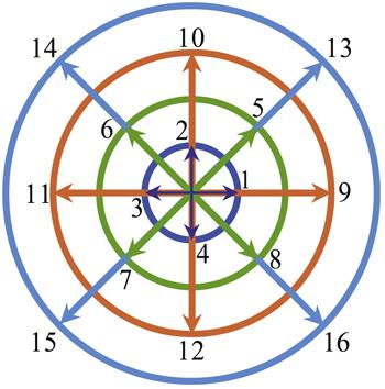
where fi and ${f}_{i}^{\mathrm{eq}}$ represent the discrete distribution function and its equilibrium counterpart, respectively. vi denotes the discrete velocity with i = 1, 2, 3, ⋯, N, and N = 16 is the total number of discrete velocities. Here a two-dimensional sixteen-velocity model is employed, see figure 1.
Physically, the DBM is approximately equivalent to a continuous fluid model plus a coarse-grained model for discrete effects. Meanwhile, the DBM is roughly equivalent to a hydrodynamic model plus a coarse-grained model of thermodynamic nonequilibrium behaviors. For the sake of recovering the NS equations in the hydrodynamic limit, the discrete equilibrium distribution functions ${f}_{i}^{\mathrm{eq}}$ are required to satisfy the following relationship
where M2, M3,1, M3 and M4,2 are the kinetic moments of the distribution functions, ${{\boldsymbol{M}}}_{2}^{\mathrm{eq}}$, ${{\boldsymbol{M}}}_{3,1}^{\mathrm{eq}}$, ${{\boldsymbol{M}}}_{3}^{\mathrm{eq}}$ and ${{\boldsymbol{M}}}_{4,2}^{\mathrm{eq}}$ denote the corresponding equilibrium counterparts, Δ2, Δ3,1, Δ3 and Δ4,2 are the differences between them. Here, Δ2 represents the viscous stress tensor and disorganized momentum flux, Δ3,1 and Δ3 are relevant to the disorganized energy fluxes. Δ4,2 is related to the flux of unnorganized energy flux.
4. Verification and validation
To verify the consistency of theoretical and numerical results of the nonequilibrium manifestations of reactive flows, firstly, we simulate a reaction process in a uniform resting system. The specific-heat ratio is γ = 5/3, the chemical heat release Q = 1, the space step Δx = Δy = 5 × 10⁻⁵, the time step Δt = 2 × 10⁻⁶, and the discrete velocities (va, vb, vc, vd, ηa, ηb, ηc, ηd) = (3.7, 3.2, 1.4, 1.4, 2.4, 0, 0, 0), respectively. In order to possess a high computational efficiency, only one mesh grid (Nx × Ny = 1 × 1) is used, and the periodic boundary condition is adopted in each direction, because the physical field is uniformly distributed. It is found that all simulated nonequilibrium physical quantities (including Δ2, Δ3,1, Δ3, and Δ4,2) remain zero during the evolution. Therefore, in the process of the chemical reaction, the deviation of velocity distribution function f from its equilibrium counterpart f eq is zero, i.e f = f eq. Besides, all physical gradients are zero in the simulation process due to the uniform distribution of physical quantities. Consequently, it is numerically verified that the chemical reaction does not contribute to the nonequilibrium effects directly1
1It should be mentioned that the chemical reaction may change the physical gradients which make an impact on the nonequilibrium effects. In other words, the chemical reaction plays an indirect role in nonequilibrium effect of the reactive flows.
(. This result is consistent with the aforementioned theory that the distribution function depends on the physical quantities and derivatives, and is independent of chemical reactions directly, see equation (13).
For the purpose of further validation, the one-dimensional (1D) steady detonation is simulated. The initial configuration, obtained from the Hugoniot relation, takes the form
where the subscript L indicates 0 ≤ x ≤ 0.00555, and R indicates 0.00555 < x ≤ 0.555. The Mach number is 1.96. To ensure the resolution is high enough, the grid is chosen as Nx × Ny = 11 100 × 1, other parameters are the same as before. Furthermore, the inflow and/or outflow boundary conditions are employed in the x direction, and the periodic boundary condition is adopted in the y direction.
Figure 2 displays the kinetic moments of velocity distribution function (M2,xx, M2,xy, M2,yy, M3,1,x, M3,1,y), the equilibrium counterparts (${M}_{2,{xx}}^{\mathrm{eq}}$, ${M}_{2,{xy}}^{\mathrm{eq}}$, ${M}_{2,{yy}}^{\mathrm{eq}}$, ${M}_{3,1,x}^{\mathrm{eq}}$, ${M}_{3,1,y}^{\mathrm{eq}}$), and the nonequilibrium quantities (Δ2,xx, Δ2,xy, Δ2,yy, Δ3,1,x, Δ3,1,y) around the detonation front. Here Δ2,xx represents twice the disorganized energy in the x degree of freedom, and Δ2,yy twice the disorganized energy in the y degree of freedom. Δ3,1,x and Δ3,1,y denote twice the disorganized energy fluxes in the x and y directions, respectively. The legends are in each plot, where the dashed line is located at the position x = 0.50375.
Figure 2. The nonequilibrium and equilibrium kinetic moments, and the differences between them. Plots (a)–(d) show the independent variables of M2 (${{\boldsymbol{M}}}_{2}^{\mathrm{eq}}$), M3,1 (${{\boldsymbol{M}}}_{3,1}^{\mathrm{eq}}$), Δ2, and Δ3,1, respectively.
In figure 2(a), the solid squares, circles and triangles stand for the DBM results of kinetic moments of distribution function M2,xx, M2,xy, and M2,yy, respectively. The hollow squares, circles and triangles represent the DBM results of the kinetic moments of equilibrium distribution function ${M}_{2,{xx}}^{\mathrm{eq}}$, ${M}_{2,{xy}}^{\mathrm{eq}}$, and ${M}_{2,{yy}}^{\mathrm{eq}}$, respectively. And the solid lines indicate the corresponding analytic solutions, ${M}_{2,{xx}}^{\mathrm{eq}}=\rho \left(T+{u}_{x}^{2}\right)$, ${M}_{2,{xy}}^{\mathrm{eq}}\,=\rho {u}_{x}{u}_{y}$, and ${M}_{2,{yy}}^{\mathrm{eq}}=\rho \left(T+{u}_{y}^{2}\right)$, respectively. With the detonation wave propagating from left to right, M2,xx, ${M}_{2,{xx}}^{\mathrm{eq}}$, M2,yy, ${M}_{2,{yy}}^{\mathrm{eq}}$ first increase due to the compressible effect, then decrease owing to the rarefaction effect, and form a peak around the detonation front. Meanwhile, M2,xy and ${M}_{2,{xy}}^{\mathrm{eq}}$ remain zero, because the detonation wave propagates forwards in the x direction. In addition, as for the equilibrium kinetic moments (${M}_{2,{xx}}^{\mathrm{eq}}$, ${M}_{2,{xy}}^{\mathrm{eq}}$, and ${M}_{2,{yy}}^{\mathrm{eq}}$), the DBM results are in good agreement with the analytical solutions.
In figure 2(b), the solid squares and circles represent M3,1,x and M3,1,y, respectively. The hallow symbols denote the equilibrium counterparts ${M}_{3,1,x}^{\mathrm{eq}}$, and ${M}_{3,1,y}^{\mathrm{eq}}$. And the solid lines indicate the analytic solutions ${M}_{3,1,x}^{\mathrm{eq}}=\rho {u}_{x}\left[\left(D+I+2\right)T+{u}^{2}\right]$ and ${M}_{3,1,y}^{\mathrm{eq}}=\rho {u}_{y}\left[\left(D+I+2\right)T+{u}^{2}\right]$. Similarly, M3,1,x and ${M}_{3,1,x}^{\mathrm{eq}}$ ascend rapidly and then decline slowly due to the compressible and rarefaction effects, respectively. M3,1,y and ${M}_{3,1,y}^{\mathrm{eq}}$ are still zero in the one-dimensional simulation.
In figure 2(c), as the detonation wave travels from left to right, Δ2,xx expressed by the solid line with squares first increases, then decreases, and increases afterwards, so it forms a high positive peak and a negative trough. Actually, figure 2(c) is consistent with figure 2(a) where M2,xx is first greater than ${M}_{2,{xx}}^{\mathrm{eq}}$ and then less than ${M}_{2,{xx}}^{\mathrm{eq}}$ as the detonation wave travels forwards. Physically, Δ2,xx stands for twice the disorganized energy in the x direction, its positive peak and the negative trough correspond to the compression and rarefaction effects, respectively. The solid line with triangles denotes twice the disorganized energy in the y direction Δ2,yy, which first decreases to form a negative trough and then increases to form a low positive peak. This trend is also consistent with the results of M2,yy and ${M}_{2,{yy}}^{\mathrm{eq}}$ in figure 2(a). Additionally, ${{\rm{\Delta }}}_{2,{xy}}={M}_{2,{xy}}-{M}_{2,{xy}}^{\mathrm{eq}}=0$ in figure 2(c) is in line with ${M}_{2,{xy}}={M}_{2,{xy}}^{\mathrm{eq}}=0$ in figure 2(a).
In figure 2(d), Δ3,1,x and Δ3,1,y denote twice the disorganized energy fluxes in the x and y directions, respectively. Δ3,1,x and Δ3,1,y are the differences between the kinetic moment M3,1,x, M3,1,y and their equilibrium counterparts ${M}_{3,1,x}^{\mathrm{eq}},{M}_{3,1,y}^{\mathrm{eq}}$, respectively. Obviously, Δ3,1,x forms a positive peak and then a low negative trough. Because the M3,1,x is first greater and then less than ${M}_{3,1,x}^{\mathrm{eq}}$. Besides, M3,1,y and ${M}_{3,1,y}^{\mathrm{eq}}$ are zero, which causes ${{\rm{\Delta }}}_{\mathrm{3,1},y}={M}_{\mathrm{3,1},y}-{M}_{3,1,y}^{\mathrm{eq}}$ to be zero as well.
Next, let us verify that the kinetic moments calculated by the summations of the discrete distribution functions are close to those calculated by integrals of their original forms at the location x = 0.50375. The kinetic moments calculated by the summations of the discrete distribution functions are (Δ2,xx, Δ2,xy, Δ2,yy, Δ3,1,x, Δ3,1,y) = (0.48449, 0, −0.35844, 2.891 23, 0), while the results of the corresponding integration counterparts are (Δ2,xx, Δ2,xy, Δ2,yy, Δ3,1,x, Δ3,1,y) = (0.56488, 0, −0.27255, 2.801 81, 0). The relative errors are (17%, 0%, 24%, 3%, 0%), which is roughly satisfactory. For the first time, this test demonstrates the accuracy of the nonequilibrium manifestations measured by the DBM, and validates the consistence of the DBM with its theoretical basis.
5. Recovery of velocity distribution function around detonation wave
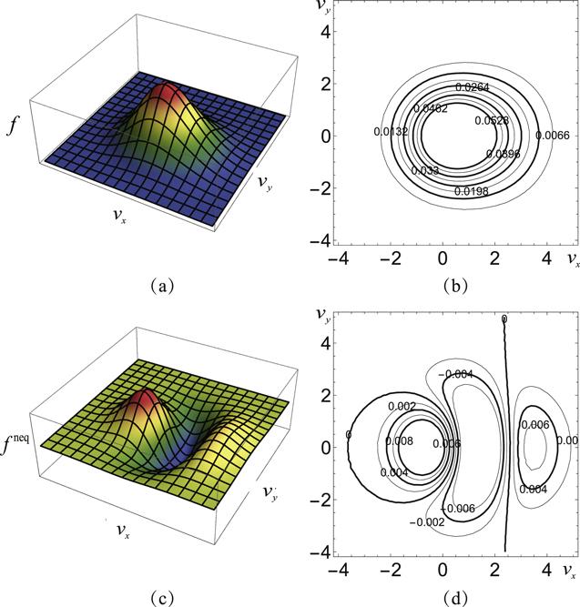
To further perform a quantitative study of the nonequilibrium state around the detonation wave, figure 3(a) displays the velocity distribution function at the peak of Δ2,xx, which is on the vertical dashed line in figure 2. It is clear that the velocity distribution function has a peak in the two-dimensional velocity space. Actually, due to the nonequilibrium effects, the velocity distribution function deviates from its local equilibrium counterpart, i.e. the Maxwellian velocity distribution function.
Figure 3. The velocity distribution function (a) and its corresponding contour(b), the deviation of the velocity distribution function from the equilibrium state (c) and its corresponding contour (d).
In order to have an intuitive study of the local velocity distribution function, figure 3(b) shows its contours in the velocity space, which is in line with figure 3(a). Clearly, the peak is asymmetric in the vx direction and symmetric in the vy direction. The contour lines are close to each other near the peak (especially on the left side), and becomes sparse away from the peak (especially on the right side). That is to say, the gradient is sharp near the peak (especially on the left side), and smooth far from the peak (especially on the left side).
To have a deep understanding of the deviation of the velocity distribution function from the equilibrium state, figure 3(c) depicts the difference between the nonequilibrium and equilibrium distribution functions in the two-dimensional velocity space. It is obvious that there are both positive and negative deviations around the detonation wave. Along the vx direction, a high positive peak first appears, then decreases to form a valley, and then increases to a low positive peak.
As can be seen in figure 3(d), the deviation is symmetric about vy = 0, and asymmetric about vx = ux. The contour plot consists of three segments along the vx direction. The leftmost segment is in the region of the first peak, where the contour lines are approximately elliptical. The middle part is in the low valley area that seems like a ‘moon’ shape. And the rightmost one is in the low peak area, which likes a ‘cobblestone’. The contour lines between the high peak and the valley are closer to each other than those between the valley and low peak, because the gradients between the leftmost and middle parts are sharp than those between the middle and rightmost regions.
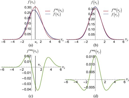
Finally, let us investigate the one-dimensional distribution functions and the corresponding deviations from the equilibrium states. Figures 4(a) and (b) depict the velocity distribution functions in the vx and vy directions, respectively. The solid lines represent the velocity distribution functions f (vx) = ∫∫ fdvydη and f(vy) = ∫∫ fdvxdη, the dashed curves express the equilibrium counterparts f eq(vx) = ∫∫ f eqdvydη and f eq(vy) = ∫∫ f eqdvxdη, respectively. Figures 4(c) and (d) show f neq(vx) = f (vx) − f eq(vx) and f neq(vy) = f(vy) − f eq(vy) which indicate the departures of distribution functions from the equilibrium state in the vx and vy directions, respectively. The following points can be obtained.
I
(I)In figures 4(a)–(b), there is a peak for each curve of f(vx), f eq(vx), f (vy), and f eq(vy). In figures 4(c)–(d), there are two peaks and a trough for f neq(vx), while a peak and two troughs for f neq(vy). Along the vx direction, f neq(vx) forms a positive peak firstly, then decreases to form a valley, and then increases to a second positive peak. Because f (vx) is first greater than f eq(vx), then less than f eq(vx), and finally greater than f eq(vx) again. Similarly, the relation f(vy) > f eq(vy) or f(vy) < f eq(vy) in figure 4(b) leads to the results f neq(vy) > 0 or f neq(vy) < 0 in figure 4(d).
II
(II)f(vx) and f neq(vx) are asymmetric about the vertical dashed line located at vx = ux, while f eq(vx) is symmetric. Physically, as the detonation evolves, the compressible effect plays a significant role in the front of the detonation wave, and the internal energy in the x degree of freedom increases faster than in other degrees of freedom, and there exists disorganized heat flux in the x direction.
III
(III)In figures 4(b) and (d), each curve of f(vy), f eq(vy) and f neq(vy) has a positive peak which is symmetric about vy = 0. On the left and right parts of f neq(vy) are two identical troughs that are symmetrically distributed in figure 4(b). Because the periodic boundary condition is imposed on the y direction, the equilibrium and nonequilibrium velocity distributions for vy > 0 and vy < 0 are symmetrical.
IV
(IV)The nonequilibrium manifestations in figures 2(a)–(d) are consistent with the deviations of distribution functions in figures 4(a)–(d). Specifically, the trend of f neq(vx) indicates that f(vx) is ‘fatter’ and ‘lower’ than f eq(vx), which means the disorganized momentum flux Δ2,xx > 0. The trend of f neq(vy) means that f(vy) is ‘thinner’ and ‘higher’ than f eq(vy), which indicates Δ2,yy < 0. Meanwhile, the portion f(vx > ux) is ‘fatter’ than the part f(vx < ux), which is named ‘positive skewness’ and indicates Δ3,1,x > 0. And the symmetry of f neq(vy) means Δ3,1,y = 0.
Figure 4. One-dimensional nonequilibrium and equilibrium distribution functions in the vx (a) and vy (b) directions, and the differences between them in the vx (c) and vy (d) directions.
6. Conclusions
Via the Chapman–Enskog expansion, the velocity distribution function of compressible reactive flows is expressed by using the macroscopic quantities and their spatial derivatives. The equilibrium and nonequilibrium distribution functions in one- and two-dimensional velocity spaces are recovered quantitatively from the physical quantities of the DBM, which is an accurate and efficient gas kinetic method. The departure between the equilibrium and nonequilibrium distribution functions is in line with the nonequilibrium quantities measured by the DBM. Moreover, it is for the first time to verify that the kinetic moments measured by summations of the distribution function resemble those assessed by integrals of the original forms, which consists with the theoretical basis of the DBM. In addition, under the condition that the chemical time scale is longer than the molecular relaxation time, it is numerically and theoretically demonstrated that the chemical reaction imposes no direct impact on the thermodynamic nonequilibrium effects.
HeZ XYanW WZhangKYangX LWeiY K2017 Simulation of effect of bottom heat source on natural convective heat transfer characteristics in a porous cavity by lattice Boltzmann method Acta Phys. Sin.66 145 153
LiCMengyiWQinjunKWenquanT2018 Pore scale study of multiphase multicomponent reactive transport during CO2 dissolution trapping Adv. Water Resour.116 208 218
WuHBergPLiX2010 Steady and unsteady 3D non-isothermal modeling of PEM fuel cells with the effect of non-equilibrium phase transfer Appl. Energy87 2778 2784
LaiHXuAZhangGGanYYingYSucciS2016 Nonequilibrium thermohydrodynamic effects on the Rayleigh–Taylor instability in compressible flows Phys. Rev. E94 023106
DubeyA KBodrovaAPuriSBrilliantovN2013 Velocity distribution function and effective restitution coefficient for a granular gas of viscoelastic particles Phys. Rev. E87 062202
WatariM2007 Finite difference lattice Boltzmann method with arbitrary specific heat ratio applicable to supersonic flow simulations Physica A382 502 522
NgH DRadulescuM IHigginsA JNikiforakisNLeeJ H S2005 Numerical investigation of the instability for one-dimensional Chapman–Jouguet detonations with chain-branching kinetics Combust. Theory Model.9 385 401


