


1. Introduction
Due to the valley degree of freedom in addition to the charge and spin of an electron, novel valleytronics that can store, manipulate and encode information rises. In two-dimensional materials, two inequivalent valleys origin from the maximum (minimum) of valence (conduction) band in the first Brillouin zone [1–9]. And the valley degree of freedom has been experimentally realized by the means, such as electric, magnetic and optical fields [10–12], which is an important platform to design valleytronics. In graphene, the valley polarized transport is theoretically proposed by the strain and magnetic field [13–16]. In recent years, valleytronics has been applied in the caloritronics called as the valley caloritronics using the thermoelectric heat to drive the valley current [17–20]. Based on the valley caloritronics, some related valley phenomena appear. For instance, the valley Seebeck effect is proposed by breaking the transmission symmetry around zero energy in the first subband of the zigzag graphene nanoribbon [20]; and the valley-locked spin-dependent Seebeck effect is discovered with a proximity-induced asymmetric magnetic field [17].
Haldane first introduced the Haldane model to realize the quantum anomalous Hall effect in the absence of external magnetic field [21], and the experimental realization of the Haldane model is first achieved by using cold atoms in a shaken optical lattice [22]. The means, such as Fe-based honeycomb ferromagnetic insulator [23] and transition-metal pnictides [24], are also proposed to realize the Haldane model. Based on the Haldane model, Colomés and Franz have theoretically proposed the modified Haldane model revealing the antichiral edge modes, where two copropagating edge modes are compensated by the bulk counterpropagating modes. Actually, the modified Haldane model might be possible with Weyl semimetals and transition metal dichalcogenides monolayers [2, 25–28]. The modified Haldane model has been used in some applications. For instance, Marc Vila obtained a rich phase diagram of optical absorption with a modified Haldane model [28], and Marwa Mannaï and Sonia Haddad obtained a strain-tunable edge current in topological insulator with a modified Haldane model [29].
In this work, we design three types of current, such as the 100% spin-valley polarized current (SVCC), pure spin-valley current (SVC) and pure charge current (CC), with a modified Haldane model under a temperature difference in a two-terminal graphene-based model. These types of current are dependent on the functions of the valley chooser and spin chooser. Modulating the phase $\phi $ and next-near-neighbor hopping ${t}_{2}$ of the modified Haldane model is an important way to obtain and mutually switch these types of current. Modulating the polarized direction of the light is also important way to obtain these currents. These results indicate that by using the modified Haldane model, a two-terminal graphene-based system can be used to design spin and valley caloritronics.
2. Model and methods
In figure 1, we theoretically propose a two-terminal graphene-based system to design three types of current. Before introducing the results, we define the direction of the current propagating from the left thermoelectrode (region I) to the right thermoelectrode (region IV) as the positive direction. In the region II called as a valley chooser, we consider a modified Haldane model and staggered potential, while in the region III called as a spin chooser, the staggered exchange interaction and off-resonant circularly polarized light are considered. Near two momentum valleys $K$ and $K^{\prime} ,$ the low-energy effective Hamiltonian can be expressed as1 ) to balance the induced staggered potential by the ferromagnetic proximity. And the exchange interaction can be expressed as ${H}_{{\rm{ex}}}={\lambda }_{{\rm{ex}}}^{A}\left({\tau }_{z}-{\tau }_{0}\right){\sigma }_{z}/2$ + ${\lambda }_{{\rm{ex}}}^{B}\left({\tau }_{z}+{\tau }_{0}\right){\sigma }_{z}/2,$ where ${{\lambda }}_{{\rm{e}}{\rm{x}}}^{A}$ and ${{\lambda }}_{{\rm{e}}{\rm{x}}}^{B}$ are the exchange interaction at the sublattices A and B, respectively. In a special case of ${{\lambda }}_{{\rm{e}}{\rm{x}}}^{A}={{\lambda }}_{{\rm{e}}{\rm{x}}}^{B},$ the fourth term appears. The fifth term arises from the case, where a beam of off-resonant circularly polarized light of $A\left(t\right)=A\left[\xi \,\sin \left(\omega t\right){e}_{x}+\,\cos \left(\omega t\right){e}_{y}\right]$ is coupled to the graphene-based model [35–37]. And ${\lambda }_{{\rm{\Omega }}}=\xi {(eA{v}_{F})}^{2}/\hslash \omega ,$ where $\xi =\pm 1$ represent the right and left polarized light. The basis of the Hamiltonian equation (1 ) is presented in detail in the appendix A .
$\begin{eqnarray}H={H}_{0}+{\rm{\Delta }}{\tau }_{z}+\left(\eta {t}_{2}^{a}+{t}_{2}^{b}\right){\tau }_{0}{\sigma }_{0}+{\lambda }_{{\rm{AF}}}{\tau }_{z}{\sigma }_{z}+\eta {\lambda }_{{\rm{\Omega }}}{\tau }_{z}{\sigma }_{0},\end{eqnarray}$
where the first term ${H}_{0}=\hslash {v}_{F}\left(\eta {\tau }_{x}{k}_{x}+{\tau }_{y}{k}_{y}\right)$ denotes pure graphene interactions in regions I and IV without external fields. ${v}_{F}=1\times {10}^{6}\,{\rm{m}}\,{{\rm{s}}}^{-1}$ represents the Fermi velocity and $\hslash $ is the reduced Plank constant. $\eta =\pm 1$ correspond to the valleys $K$ and $K^{\prime} ,$ ${\tau }_{i}$ and ${\sigma }_{i}$ with the index $i=x,\,y,\,z$ describe the sublattice and spin Pauli matrices, respectively. Besides, ${\tau }_{0}$ and ${\sigma }_{0}$ are the corresponding unit Pauli matrices. The second term denotes the staggered potential, which can be obtained by putting the graphene-based model on an h-BN substrate [30, 31], the third term denotes the modified Haldane model, where ${t}_{2}^{a}=-3\sqrt{3}{t}_{2}\,\sin \,\phi $ and ${t}_{2}^{b}=-3{t}_{2}\,\cos \,\phi .$ In addition, some possible schemes have been proposed to obtain the modified Haldane model in graphene [25, 28]. The fourth term represents the staggered exchange interaction, which can be hardly realized in planar structure such as graphene. We proposed an appropriate method that depend on the bulk or planar structure to induced staggered interaction. Based on the ab initio calculations [32], the exchange interaction and staggered potential emerge as the graphene is put on the hexagonal BN planar deposited on ferromagnetic Co or Ni [33] or the hBN/(Co, Ni) [34]. For the purpose of obtaining the exchange interaction, one can use the staggered potential of the second term of equation (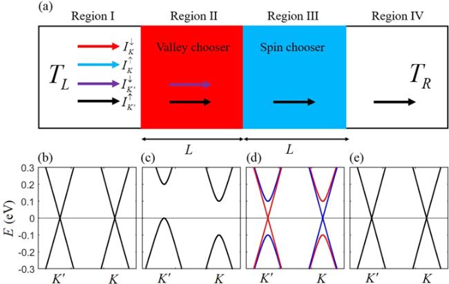
Figure 1. (a) Schematic illustration of a two-terminal graphene-based system with left and right thermoelectrodes that have a kinetic energy difference ${\rm{\Delta }}\omega ={k}_{B}{T}_{L}-{k}_{B}{T}_{R}=0.005\,{\rm{eV}},$ the widths of regions II and III are set as $L.$ The energy bands in figures (b)–(e) correspond to regions I–IV, respectively. In the energy bands, the red and blue lines denote the spin-up and spin-down modes, respectively, and the black line denotes the degeneracy of the spin. In the region II, $\phi =5\pi /6,$ ${t}_{2}=\sqrt{3}/90\,{\rm{eV}}$ and ${\rm{\Delta }}=0.1\,{\rm{eV}}.$ In region III, ${\lambda }_{{\rm{\Omega }}}=0.05\,{\rm{eV}}$ and ${\lambda }_{{\rm{AF}}}=0.05\,{\rm{eV}}.$ In regions I and IV, no external fields exist. |
From the Hamiltonian (1 ), we can easily obtain the eigenvalues2 ), the corresponding wave function with a given energy $E$ can be derived as
$\begin{eqnarray}{E}_{\xi \eta S}=\eta {t}_{2}^{a}+{t}_{2}^{b}\pm \sqrt{{\left(\hslash {v}_{F}\right)}^{2}+{\left({\rm{\Delta }}+S{\lambda }_{{\rm{AF}}}+\eta {\lambda }_{{\rm{\Omega }}}\right)}^{2}},\end{eqnarray}$
where the signs $\pm $ denote the conduction and valence bands, respectively. The variable $S=\pm 1$ are defined for the spin-up and spin-down modes, respectively. Based on the equation ( $\begin{eqnarray}\begin{array}{l}{\varphi }_{1}=\left(\begin{array}{c}1\\ \displaystyle \frac{E}{\hslash {v}_{F}\left(\eta {k}_{x1}-{\rm{i}}{k}_{y1}\right)}\end{array}\right){{\rm{e}}}^{{\rm{i}}{k}_{x1} \ x}\\ \,+{r}_{1}\left(\begin{array}{c}1\\ \displaystyle \frac{E}{\hslash {v}_{F}\left(-\eta {k}_{x1}-{\rm{i}}{k}_{y1}\right)}\end{array}\right){{\rm{e}}}^{-{\rm{i}}{k}_{x1} \ x},\\ {\varphi }_{2}={t}_{2}\left(\begin{array}{c}1\\ \displaystyle \frac{E-{\rm{\Delta }}-\eta {t}_{2}^{a}-{t}_{2}^{b}}{\hslash {v}_{F}\left(\eta {k}_{x2}-{\rm{i}}{k}_{y2}\right)}\end{array}\right){{\rm{e}}}^{{\rm{i}}{k}_{x2} \ x}\\ \,+{r}_{2}\left(\begin{array}{c}1\\ \displaystyle \frac{E-{\rm{\Delta }}-\eta {t}_{2}^{a}-{t}_{2}^{b}}{\hslash {v}_{F}\left(-\eta {k}_{x2}-{\rm{i}}{k}_{y2}\right)}\end{array}\right){{\rm{e}}}^{-{\rm{i}}{k}_{x2} \ x},\\ {\varphi }_{3}={t}_{3}\left(\begin{array}{c}1\\ \displaystyle \frac{E-S{\lambda }_{{\rm{AF}}}-\eta {\lambda }_{{\rm{\Omega }}}}{\hslash {v}_{F}\left(\eta {k}_{x3}-{\rm{i}}{k}_{y3}\right)}\end{array}\right){{\rm{e}}}^{{\rm{i}}{k}_{x3} \ x}\\ \,+{r}_{3}\left(\begin{array}{c}1\\ \displaystyle \frac{E-S{\lambda }_{{\rm{AF}}}-\eta {\lambda }_{{\rm{\Omega }}}}{\hslash {v}_{F}\left(-\eta {k}_{x3}-{\rm{i}}{k}_{y3}\right)}\end{array}\right){{\rm{e}}}^{-{\rm{i}}{k}_{x3} \ x},\\ {\varphi }_{4}={t}_{4}\left(\begin{array}{c}1\\ \displaystyle \frac{E}{\hslash {v}_{F}\left(\eta {k}_{x4}-{\rm{i}}{k}_{y4}\right)}\end{array}\right){{\rm{e}}}^{{\rm{i}}{k}_{x4} \ x},\end{array}\end{eqnarray}$
where the indices $i=1,2,3,4$ of the wave function ${\varphi }_{i}$ represent the regions I–IV, respectively. In the same case, the indices ${t}_{i}$ and ${r}_{i}$ denote the transmission and reflection coefficients in the corresponding regions, respectively. In addition, ${k}_{xi}$ and ${k}_{yi}$ are the wavevectors.Here, we use the transfer matrix method to obtain the total transmission. By using the continuity condition of the wave functions at each interface between nearest regions, we can get simple formulas at each interface as4 ) can be reduced asB . Furthermore, the total spin-valley transmission probability with incident angle $\theta $ is expressed as
$\begin{eqnarray}{M}_{1}\left[\begin{array}{c}1\\ {r}_{1}\end{array}\right]={M}_{2}\left[\begin{array}{c}{t}_{2}\\ {r}_{2}\end{array}\right],{M}_{3}\left[\begin{array}{c}{t}_{2}\\ {r}_{2}\end{array}\right]={M}_{4}\left[\begin{array}{c}{t}_{3}\\ {r}_{3}\end{array}\right],{M}_{5}\left[\begin{array}{c}{t}_{3}\\ {r}_{3}\end{array}\right]={M}_{6}\left[\begin{array}{c}{t}_{4}\\ 0\end{array}\right],\end{eqnarray}$
where the matrices ${M}_{i}$ are expressed as $\begin{eqnarray}\begin{array}{l}{M}_{1}=\left[\begin{array}{cc}1 & 1\\ \displaystyle \frac{E}{\hslash {v}_{F}\left(\eta {k}_{x1}-{\rm{i}}{k}_{y1}\right)} & \displaystyle \frac{E}{\hslash {v}_{F}\left(-\eta {k}_{x1}-{\rm{i}}{k}_{y1}\right)}\end{array}\right],\\ {M}_{2}=\left[\begin{array}{cc}1 & 1\\ \displaystyle \frac{E-{\rm{\Delta }}-\eta {t}_{2}^{a}-{t}_{2}^{b}}{\hslash {v}_{F}\left(\eta {k}_{x2}-{\rm{i}}{k}_{y2}\right)} & \displaystyle \frac{E-{\rm{\Delta }}-\eta {t}_{2}^{a}-{t}_{2}^{b}}{\hslash {v}_{F}\left(-\eta {k}_{x2}-{\rm{i}}{k}_{y2}\right)}\end{array}\right],\\ {M}_{3}=\left[\begin{array}{cc}{{\rm{e}}}^{{\rm{i}}{k}_{x2}L} & {{\rm{e}}}^{-{\rm{i}}{k}_{x2}L}\\ \displaystyle \frac{E-{\rm{\Delta }}-\eta {t}_{2}^{a}-{t}_{2}^{b}}{\hslash {v}_{F}\left(\eta {k}_{x2}-{\rm{i}}{k}_{y2}\right)}{{\rm{e}}}^{{\rm{i}}{k}_{x2}L} & \displaystyle \frac{E-{\rm{\Delta }}-\eta {t}_{2}^{a}-{t}_{2}^{b}}{\hslash {v}_{F}\left(-\eta {k}_{x2}-{\rm{i}}{k}_{y2}\right)}{{\rm{e}}}^{-{\rm{i}}{k}_{x2}L}\end{array}\right],\\ {M}_{4}=\left[\begin{array}{cc}{{\rm{e}}}^{{\rm{i}}{k}_{x3}L} & {{\rm{e}}}^{-{\rm{i}}{k}_{x3}L}\\ \displaystyle \frac{E-S{\lambda }_{{\rm{AF}}}-\eta {\lambda }_{{\rm{\Omega }}}}{\hslash {v}_{F}\left(\eta {k}_{x3}-{\rm{i}}{k}_{y3}\right)}{{\rm{e}}}^{{\rm{i}}{k}_{x3}L} & \displaystyle \frac{E-S{\lambda }_{{\rm{AF}}}-\eta {\lambda }_{{\rm{\Omega }}}}{\hslash {v}_{F}\left(-\eta {k}_{x3}-{\rm{i}}{k}_{y3}\right)}{{\rm{e}}}^{-{\rm{i}}{k}_{x3}L}\end{array}\right],\\ {M}_{5}=\left[\begin{array}{cc}{{\rm{e}}}^{{\rm{i}}{k}_{x3}2L} & {{\rm{e}}}^{-{\rm{i}}{k}_{x3}2L}\\ \displaystyle \frac{E-S{\lambda }_{{\rm{AF}}}-\eta {\lambda }_{{\rm{\Omega }}}}{\hslash {v}_{F}\left(\eta {k}_{x3}-{\rm{i}}{k}_{y3}\right)}{{\rm{e}}}^{{\rm{i}}{k}_{x3}2L} & \displaystyle \frac{E-S{\lambda }_{{\rm{AF}}}-\eta {\lambda }_{{\rm{\Omega }}}}{\hslash {v}_{F}\left(-\eta {k}_{x3}-{\rm{i}}{k}_{y3}\right)}{{\rm{e}}}^{-{\rm{i}}{k}_{x3}2L}\end{array}\right],\\ {M}_{6}=\left[\begin{array}{cc}{{\rm{e}}}^{{\rm{i}}{k}_{x4}2L} & 0\\ \displaystyle \frac{E}{\hslash {v}_{F}\left(\eta {k}_{x4}-{\rm{i}}{k}_{y4}\right)}{{\rm{e}}}^{{\rm{i}}{k}_{x4}2L} & 0\end{array}\right].\end{array}\end{eqnarray}$
It is obvious that the rearranged formula for the equation ( $\begin{eqnarray}\left[\begin{array}{c}1\\ {r}_{1}\end{array}\right]=M\left[\begin{array}{c}{t}_{4}\\ 0\end{array}\right],\end{eqnarray}$
with the total transfer matrix $M={M}_{1}^{-1}{M}_{2}{M}_{3}^{-1}{M}_{4}{M}_{5}^{-1}{M}_{6}$ [38]. Then, the transmission coefficient is easily derived as ${t}_{4}=\tfrac{1}{{M}_{11}},$ where ${M}_{11}$ is the element of the total transfer matrix $M.$ The spin-valley dependent transmission probability is also easily obtained as $\begin{eqnarray}{T}_{\eta S}=\displaystyle \frac{1}{{{M}_{11}}^{\ast }{M}_{11}},\end{eqnarray}$
this formula is suitable for the case, where the left and right thermoelectrodes are symmetrical. In addition, another method for calculating the transmission coefficient ${t}_{4}$ is presented in the appendix $\begin{eqnarray}{T}_{\eta S}^{{\rm{total}}}\left(E\right)=\displaystyle \frac{\lambda W}{\hslash {v}_{F}\pi }\displaystyle \frac{\hslash {v}_{F}k}{\lambda }\displaystyle {\int }_{-\displaystyle \frac{\pi }{2}}^{\displaystyle \frac{\pi }{2}}{T}_{\eta S}\,\cos \,\theta {\rm{d}}\theta ,\end{eqnarray}$
with large enough width $W$ of graphene-based system. We introduce the energy scale $\lambda =0.0039\,{\rm{eV}}$ to make these terms $\lambda W/\hslash {v}_{F}\pi $ and $\hslash {v}_{F}k/\lambda $ dimensionless. In addition, this term $\hslash {v}_{F}k/\lambda $ is dimensionless variable due to the wavevector $k.$ And the incident angle $\theta $ satisfies the condition of $\theta =\arctan \left({k}_{y1}/{k}_{x1}\right).$ After obtaining the total transmission probability, one can get the formula of the spin-valley current by using the generalized Landauer–Büttiker transport approach as $\begin{eqnarray}{I}_{\eta }^{S}=\displaystyle \frac{e\lambda W}{{\hslash }^{2}{\pi }^{2}{v}_{F}}\displaystyle \int {\rm{d}}E{\rm{\Delta }}{f}_{{\rm{LR}}}\displaystyle \frac{\hslash {v}_{F}k}{\lambda }\displaystyle {\int }_{-\displaystyle \frac{\pi }{2}}^{\displaystyle \frac{\pi }{2}}{T}_{\eta S}\left(\theta \right)\cos \,\theta {\rm{d}}\theta ,\end{eqnarray}$
where we define the term ${I}_{0}=\tfrac{e\lambda W}{{\hslash }^{2}{\pi }^{2}{v}_{F}}$ as a unit of the spin-valley current ${I}_{\eta }^{S}.$${\rm{\Delta }}f={f}_{L}-{f}_{R}$ is the Fermi function difference between left and right thermoelectrodes, where the Fermi function $f=1/\left\{\exp \left[\left(E-{E}_{f}\right)/{k}_{B}T\right]+1\right\}$ with the chemical potential ${E}_{f}=0.$ The spin, valley and charge currents are given as ${J}_{S}={J}_{\uparrow }-{J}_{\downarrow },$ ${J}_{V}={J}_{K}-{J}_{K^{\prime} }$ and ${J}_{C}={J}_{\uparrow }+{J}_{\downarrow }\,({J}_{K}+{J}_{K^{\prime} }).$ And we introduce the quantities ${P}_{S}=\tfrac{\left|{J}_{\uparrow }\right|-\left|{J}_{\downarrow }\right|}{\left|{J}_{\uparrow }\right|+\left|{J}_{\downarrow }\right|}$ and ${P}_{V}=\tfrac{\left|{J}_{K}\right|-\left|{J}_{K^{\prime} }\right|}{\left|{J}_{K}\right|+\left|{J}_{K^{\prime} }\right|}$ to calculate the spin and valley polarizations, respectively. In addition, we define a kinetic energy difference as ${\rm{\Delta }}\omega ={k}_{B}{T}_{L}-{k}_{B}{T}_{R}.$
3. Results and discussion
As we know, the size effect has an important influence on the transport property, which can be ignored by choosing an appropriate size. Before analyzing three types of current arising from a temperature difference, the effect of different widths of the regions II and III on the transport property has been discussed below. According to equation (8 ), the total spin-valley transmission can be calculated easily, which corresponds to the model shown in figure 1. From figures 2(a)–(d), it reveals that the gaps of those transmissions tend to be a steady region with the increasing widths of the regions II and III. We find that the total transmission gaps in figure 2(d) are well consistent with the energy band gaps in figures 1(b)–(d) as the length exceeds a certain value, such as $L=150a.$ Therefore, we choose the appropriate length as $L=150a$ to calculate the transport property in the following. Besides, all these total transmissions are based on the model in figure 1.
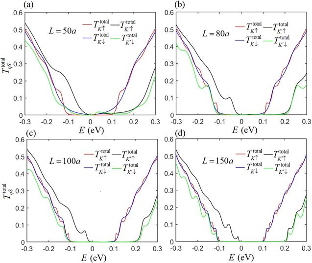
Figure 2. Transmissions with different width $L$ of regions II and III, $a$ is the lattice constant of graphene. |
In figure 1(a), we modulate the phase $\phi $ of the modified Haldane model in the region II to obtain 100% spin-valley polarized current (SVPC) shown in figures 3(e) and (f), which can be used as a spin-valley filter. Before we give a detailed discussion on the 100% SVPC, the character of the Fermi function should be simply described. According to the calculation of the Fermi function, the states can be excited about the region of $-7{k}_{{\rm{B}}}T\,\leqslant E-{E}_{f}\,\leqslant 7{k}_{{\rm{B}}}T$ by the temperature, which is important for explaining the results in the following. In the region of $0\leqslant {k}_{B}{T}_{R}\leqslant 0.01\,{\rm{eV}},$ there exist the spin and valley currents, while the absolute values of the spin and valley polarizations are both 1, which is called as 100% SVPC shown in figure 3(e). We can use the induced formula ${I}_{\eta }^{S}=\tfrac{e}{h}\displaystyle {\sum }_{E}{T}_{\eta S}^{{\rm{total}}}{\rm{\Delta }}f{\rm{d}}E$ rewritten from equation (9 ) to explain these phenomena. In the region of $0\leqslant {k}_{{\rm{B}}}{T}_{R}\lt 0.01\,{\rm{eV}},$ the states can be excited for the region of $-7{k}_{{\rm{B}}}{T}_{L}\,\lt E-{E}_{f}\,\lt 7{k}_{{\rm{B}}}{T}_{L}$ $(-0.102\,{\rm{eV}}\lt E-{E}_{f}\lt 0.102\,{\rm{eV}}).$ In figures 1(d) and 3(a), it is clearly shown that the Fermi function difference for the spin-up mode with the valley $K^{\prime} $ satisfies the case, where ${\rm{\Delta }}f\lt 0$ under ${\rm{0}}\lt E\lt 0.102\,{\rm{eV}}$ due to the excited states and ${\rm{\Delta }}f=0$ under $E\,\geqslant 0.2\,{\rm{eV}}$ or $E\leqslant 0.102\,{\rm{eV}}$ due to no excited states. Moreover, the total transmission also satisfies the case, where ${T}_{K\uparrow }^{{\rm{total}}}=0$ under $0\leqslant E\leqslant 0.2\,{\rm{eV}}$ due to the gap effect and ${T}_{K\uparrow }^{{\rm{total}}}\ne {\rm{0}}$ under $E\,\lt 0$ due to the specific spin-matching tunneling. Thus, the current ${I}_{K^{\prime} }^{\uparrow }$ is opposite according to the reduced formula ${I}_{\eta }^{S}=\displaystyle \frac{e}{h}\displaystyle {\sum }_{E}{T}_{\eta S}^{{\rm{total}}}{\rm{\Delta }}f{\rm{d}}E.$ At ${k}_{{\rm{B}}}{T}_{R}=0.01\,{\rm{eV}},$ a little state with spin-down mode can be excited in the valley $K^{\prime} $ as a result of that the excited state region of $-0.102\,{\rm{eV}}\leqslant E-{E}_{f}\leqslant 0.102\,{\rm{eV}}$ exceeds the boundary of the gap of $[-0.1\,{\rm{eV}},0.2\,{\rm{eV}}].$ And the currents with the valley $K$ are also zeros as a result of the symmetric bands in the valley $K$ [9]. Thus, the valley current ${J}_{V}$ is positive and the spin current ${J}_{S}$ is negative in the region of ${k}_{B}{T}_{R}\leqslant 0.01\,{\rm{eV}}.$ Meanwhile, the value of ${P}_{S}$ is almost 0.99, which can be regarded as a critical value of the 100% SVPC. In the region of ${k}_{{\rm{B}}}{T}_{R}\gt 0.01\,{\rm{eV}},$ the current ${I}_{K^{\prime} }^{\downarrow }$ emerges due to the larger temperature broadening. Therefore, the value of the spin polarization is obviously less than 1, while the value of the valley polarization is not changed. Compared with the case in figure 3(c), the spin and valley currents are strengthened as a function of the kinetic energy difference ${\rm{\Delta }}\omega $ shown in figure 3(d), which is also called as 100% SVPC in the region of $0\lt {\rm{\Delta }}\omega \leqslant 0.011\,{\rm{eV}}.$ At ${\rm{\Delta }}\omega =0.011\,{\rm{eV}},$ a little state with the spin-up mode can be excited in the valley $K^{\prime} ,$ but the error of the valley polarization is inside 1% from 1, which is safe to be called as the 100% SVPC.
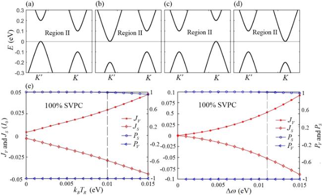
Figure 3. Band structures in region II shown in figure 1(a) and the corresponding quantities ${J}_{S},{J}_{V},{P}_{S}$ and ${P}_{V}.$ (a) $\phi =5\pi /6,$ (b) $\phi =\pi /6,$ (c) $\phi =-5\pi /6,$ (d) $\phi =-\pi /6.$ (e) The quantities ${J}_{S},{J}_{V},{P}_{S}$ and ${P}_{V}$ as a function of ${k}_{{\rm{B}}}{T}_{R}$ with respect to the band structure (a). (f) The quantities ${J}_{S},{J}_{V},{P}_{S}$ and ${P}_{V}$ as a function of ${\rm{\Delta }}\omega $ with a fixed ${k}_{B}{T}_{R}=0.005\,{\rm{eV}}$ with respect to the band structure (a). |
In the region II, we modulate the phase as $\phi =\pi /6$ instead of $\phi =5\pi /6,$ and the corresponding band structure shown in figure 3(b) implies that the direction of the 100% SVPC is opposite, which can filter the spin-up current with the valley $K^{\prime} .$ The phase $\phi $ is further modulated as $-5\pi /6$ shown in figure 3(c), which means the 100% SVPC can filter the spin-down current with the valley $K.$ And the direction of this current can be opposite by modulating the phase as $\phi =-\pi /6$ shown in figure 3(d). In the region III shown in figure 1(a), when we modulate the polarized direction of the light from the right to the left, the bands in the valleys $K$ and $K^{\prime} $ shown in figure 1(d) are interchanged not shown here. Therefore, the 100% SVPC can also filter the spin-up current with the valley $K$ and the spin-down current with the valley $K^{\prime} .$
The 100% SVPC can be switched into the pure spin-valley current (SVC), where there exist spin and valley currents and the corresponding polarizations is 0, by modulating the phase $\phi $ as $\pm \pi /2$ in the region II. In the region of $0\leqslant {k}_{{\rm{B}}}{T}_{R}\lt 0.01\,{\rm{eV}},$ only the states with spin-up mode in the valley $K^{\prime} $ are excited below ${E}_{f}$ due to the overlarge band gap of $[0,\,0.2\,{\rm{eV}}],$ while the states with spin-down mode in the valley $K$ are exited above ${E}_{f}$ due to the overlarge band gap of $[-0.2\,{\rm{eV}},\,0]$ shown in figure 4(a), which means the currents ${I}_{K^{\prime} }^{\uparrow }$ and ${I}_{K}^{\downarrow }$ contribute to the transport. At ${k}_{B}{T}_{R}=0.01\,{\rm{eV}},$ the excited state region is $-7{k}_{{\rm{B}}}{T}_{L}\,\leqslant E-{E}_{f}\,\leqslant 7{k}_{{\rm{B}}}{T}_{L}$ $(-0.102\,{\rm{eV}}\,\leqslant E-{E}_{f}\,\leqslant 0.102\,{\rm{eV}})$ beyond the boundary of the gaps of $[-0.1\,{\rm{eV}},0.2\,{\rm{eV}}]$ and $[-0.2\,{\rm{eV}},0.1\,{\rm{eV}}]$ shown in figures 1(d) and 4(a). Therefore, small amount of the currents ${I}_{K^{\prime} }^{\downarrow }$ and ${I}_{K}^{\uparrow }$ can also contribute to the transport. The values of ${P}_{V}$ and ${P}_{S}$ are almost 0.002 at ${k}_{{\rm{B}}}{T}_{R}=0.01\,{\rm{eV}}$ shown in figure 4(b), which means the value of $| {I}_{K^{\prime} }^{\uparrow }+{I}_{K}^{\uparrow }| $ is not absolutely equal to $| {I}_{K^{\prime} }^{\downarrow }+{I}_{K}^{\downarrow }| $ and the value of $| {I}_{K}^{\downarrow }+{I}_{K}^{\uparrow }| $ is not absolutely equal to $| {I}_{K^{\prime} }^{\downarrow }+{I}_{K^{\prime} }^{\uparrow }| .$ Actually, the value ${k}_{B}{T}_{R}=0.01\,{\rm{eV}}$ can be regarded as a critical value of the pure SVC. The pure SVC can be strengthened by increasing the kinetic energy difference ${\rm{\Delta }}\omega $ shown in figure 4(d). At ${\rm{\Delta }}\omega =0.011\,{\rm{eV}},$ the values of ${P}_{V}$ and ${P}_{S}$ are almost 0.002, which can be regarded as a critical value of pure SVC.
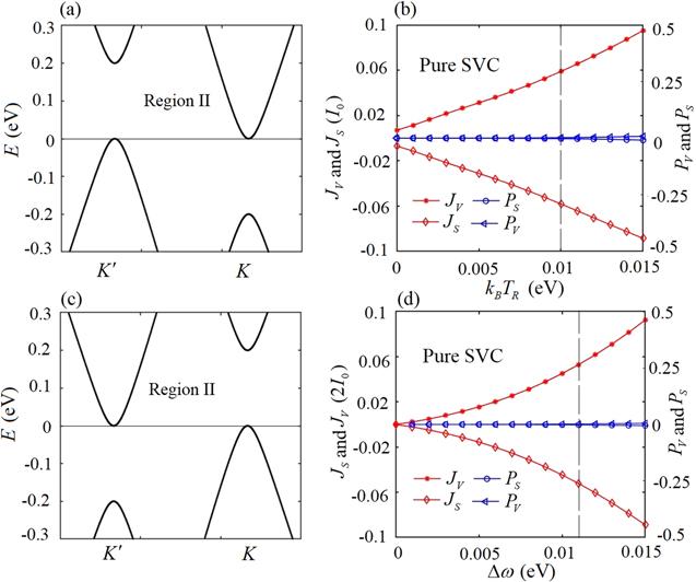
Figure 4. Band structures and the corresponding quantities ${J}_{S},{J}_{V},{P}_{S}$ and ${P}_{V}.$ (a) $\phi =\pi /2,$ (b) The quantities ${J}_{S},{J}_{V},{P}_{S}$ and ${P}_{V}$ as a function of ${k}_{{\rm{B}}}{T}_{R}$ with respect to the band structure (a), (c) $\phi =-\pi /2$. (d) The quantities ${J}_{S},{J}_{V},{P}_{S}$ and ${P}_{V}$ as a function of ${\rm{\Delta }}\omega $ with a fixed ${k}_{{\rm{B}}}{T}_{R}=0.005\,{\rm{eV}}$ with respect to the band structure (c). |
We modulate the phase as $\phi =-\pi /2$ shown in figure 4(c), the direction of the pure SVC can be opposite not shown here. In the region III shown in figure 1(a), we also modulate the polarized direction of the light from the right to the left, so that a spin chooser selects different spin modes in the same valley. Then, another two forms of the pure SVC emerge not shown here.
We further modulate the phase as $\phi =\pm \pi $ and next-near-neighbor hopping as ${t}_{2}=1/30\,{\rm{eV}}$ in the region II, then the pure SVC can be switched into the pure charge current (CC) shown in figures 5(b) and (d). In figures 5(a) and 1(d), there exist four gaps for four types of the bands, such as $[0,\,0.2\,{\rm{eV}}],\,[0,\,0.2\,{\rm{eV}}],\,[-0.1\,{\rm{eV}},\,0.2\,{\rm{eV}}]$ and $[-0.1\,{\rm{eV}},\,0.2\,{\rm{eV}}].$ It is shown that at ${k}_{B}{T}_{R}=0.01\,{\rm{eV}}$ the currents ${I}_{K^{\prime} }^{\uparrow },{I}_{K}^{\uparrow },{I}_{K^{\prime} }^{\downarrow }$ and ${I}_{K^{\prime} }^{\uparrow }$ can contribute to the transport due to the larger temperature broadening. In figure 5(b), the values of ${P}_{V}$ and ${P}_{S}$ are almost 0.002 at ${k}_{B}{T}_{R}=0.01\,{\rm{eV}},$ which can be regarded as a critical value of the pure CC. Compared with the case in figure 5(b), the pure CC can be strengthened by increasing the kinetic energy difference ${\rm{\Delta }}\omega $ shown in figure 5(d). The values of ${P}_{V}$ and ${P}_{S}$ are also 0.002 at ${\rm{\Delta }}\omega =0.011\,{\rm{eV}},$ which can be regarded as a critical value of the pure CC. We also modulate the phase as $\phi =0$ shown in figure 5(c), corresponding to the opposite direction of the pure CC shown in figure 5(b).
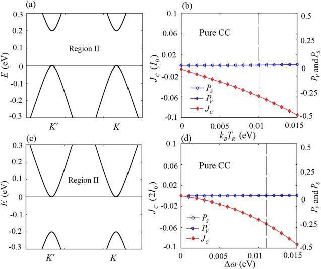
Figure 5. Band structures and the corresponding quantities ${J}_{S},{J}_{V},{P}_{S}$ and ${P}_{V}.$ (a) $\phi =\pm \pi $ and ${t}_{2}=1/30\,{\rm{eV}}.$ (b) The quantities ${J}_{S},{J}_{V},{P}_{S}$ and ${P}_{V}$ as a function of ${k}_{{\rm{B}}}{T}_{R}$ with respect to the band structure (a), (c) $\phi =0$ and ${t}_{2}=1/30\,{\rm{eV}}$. (d) The quantities ${J}_{S},{J}_{V},{P}_{S}$ and ${P}_{V}$ as a function of ${\rm{\Delta }}\omega $ with a fixed ${k}_{{\rm{B}}}{T}_{R}=0.005\,{\rm{eV}}$ with respect to the band structure (c). |
Here, we just pay attention to the off-on state of these types of current, such as the 100% SVPC, pure SVC and pure CC. It is required a long time to turn off the states by canceling the kinetic energy difference [39–41], which is a low efficiency. We find that these types of the current can be turned off by the off-resonant circularly polarized light. The currents ${J}_{\alpha }$ in figures 6(a)–(c) correspond to the cases in figures 3(a)–5(a), respectively. In figure 6, the off states are in the region of $| {\lambda }_{{\rm{\Omega }}}| \geqslant {\rm{0.12}}\,{\rm{eV}}$ as a result of that the excited state region of $-7{k}_{{\rm{B}}}{T}_{L}\lt E\,-{E}_{f}\lt 7{k}_{{\rm{B}}}{T}_{L}$$(-{\rm{0.07}}\,{\rm{eV}}\lt E-{E}_{f}\lt 0.07\,{\rm{eV}})$ is inside four gaps such as ${E}_{K}^{\uparrow },\,{E}_{K^{\prime} }^{\uparrow },\,{E}_{K}^{\downarrow },$ ${E}_{K^{\prime} }^{\downarrow }.$ And the critical value ${\lambda }_{{\rm{\Omega }}}$ of the off state satisfies the simple formula ${\lambda }_{{\rm{\Omega }}}={\lambda }_{{\rm{AF}}}+7{k}_{{\rm{B}}}{T}_{L}.$
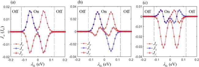
Figure 6. Currents ${J}_{\alpha }$ as a function of ${\lambda }_{{\rm{\Omega }}}$ with a fixed ${k}_{{\rm{B}}}{T}_{L}=0.01\,{\rm{eV}}$ and ${k}_{{\rm{B}}}{T}_{R}=0.005\,{\rm{eV}}$ (a) corresponds to the case in figures 2(a), (b) corresponds to the case in figures 3(a), (c) corresponds to the case in figure 4(a). |
4. Conclusion
In summary, we propose a two-terminal graphene-based system with four regions to generate three types of thermoelectric current. And these currents stem from the functions of a valley chooser and spin chooser, as well as the temperature difference. By just modulating the modified Haldane model in the region II while other parameters are kept unchanged, these types of current can be obtained and mutually switched. Moreover, the on states can be efficiently turned off by increasing the circularly polarized light intensity.