Based on the Hirota’s method, the multiple-pole solutions of the focusing Schrödinger equation are derived directly by introducing some new ingenious limit methods. We have carefully investigated these multi-pole solutions from three perspectives: rigorous mathematical expressions, vivid images, and asymptotic behavior. Moreover, there are two kinds of interactions between multiple-pole solutions: when two multiple-pole solutions have different velocities, they will collide for a short time; when two multiple-pole solutions have very close velocities, a long time coupling will occur. The last important point is that this method of obtaining multiple-pole solutions can also be used to derive the degeneration of N-breather solutions. The method mentioned in this paper can be extended to the derivative Schrödinger equation, Sine-Gorden equation, mKdV equation and so on.
Zhao Zhang, Junchao Chen, Qi Guo. Multiple-pole solutions and degeneration of breather solutions to the focusing nonlinear Schrödinger equation[J]. Communications in Theoretical Physics, 2022, 74(4): 045002. DOI: 10.1088/1572-9494/ac5cb1
1. Introduction
Nonlinear partial differential equations are often used to model various phenomena in fields such as physics, chemistry, biology and even social sciences [1–11]. With the help of exact solutions, various nonlinear phenomena can be better explained [1–7]. The construction of exact solutions of nonlinear equations, especially soliton solutions [12–14], is one of the most important and essential tasks in nonlinear science.
It is well known that the famous focusing nonlinear Schrödinger equation (FNLS equation for short)
can be used to describe optical solitons, self-trapping phenomena of nonlinear optics, propagation of thermal pulses in solids, Langnui waves in plasma, the motion of superconducting electrons in electromagnetic fields, Bose–Einstein condensation effect of atoms in lasers, and so on [15–17].
There have been hundreds of studies and monographs on how to find solutions to equation (1) [18–34]. N-soliton solutions, breather solutions, rogue wave solutions, and multiple-pole solutions of the FNLS equation have been derived by Darboux transformation, inverse scattering and other approaches [23–30]. In particular, a very mature mechanism has been developed for obtaining multiple-pole solutions, higher-order rogue wave solutions and rogue waves with a double-periodic background using the Darboux transformation [25–30].
The multiple-pole solution is actually a weakly bound state of solitons, where the velocities and amplitudes of the solitons are almost the same. In this weakly bound state, the soliton travels along a curve, and the velocity and amplitude tend to be fixed values when the time is large enough. As with the multiple-pole solutions, similar asymptotic behavior exists for degeneration of breather solutions. As early as last century, it was reported that multiple-pole solutions of the FNLS equation were obtained by the inverse scattering method [31, 32]. In 2017, Schiebold [23] produced an important work that gave a rigorous and complete asymptotic description of the multiple-pole solutions for the FNLS equation. In the same year, Wang et al [29] first discovered the degeneration of N-breather solutions using the generalized Darboux transformation and creatively pointed out the connection between it and higher-order rogue waves. Subsequently, some scholars linked the inverse scattering method [24] or the Darboux transformation method [33] to the Riemann–Hilbert problem to explore the higher-order multiple-pole solutions.
In short, most of the research to obtain the multiple-pole solution still use the inverse scattering method [23, 24, 31, 32] and Darboux transformation method [33, 34] which have higher requirements on mathematics.
However, there is no report on whether the Hirota’s method [14, 35–40], as a direct method to obtain the exact solution of the integrable system, can derive the multiple-pole solution of FNLS equation. According to the bilinear method, the N-soliton solution of the FNLS equation takes the following form [19, 20, 41]:
Here ${A}_{1}\left(\mu \right)$ and ${A}_{2}\left(\mu \right)$ are the summation over all possible combinations of μ1 = {0, 1}, μ2 = {0, 1}, ⋯, μ2N = {0, 1}. Moreover, ${A}_{1}\left(\mu \right)$ and ${A}_{2}\left(\mu \right)$ also satisfy conditions ${\sum }_{j=1}^{N}{\mu }_{j}={\sum }_{j=1}^{N}{\mu }_{N+j}$ and ${\sum }_{j=1}^{N}{\mu }_{j}={\sum }_{j=1}^{N}{\mu }_{N+j}+1$, respectively. Note that ${\xi }_{j}^{(0)}$ is a real parameter that describes the initial position of the soliton.
The latest research [42] mentions a way to derive multiple-pole solutions directly from N-soliton solutions, which provides a possibility to concisely derive degenerate solutions from equation (2). After tedious verification, the idea mentioned in [42] is feasible for the FNLS equation. In other words, the multiple-pole solutions of equation (1) can be obtained by the Hirota’s bilinear method. Similarly, degenerate solutions can be derived directly from N-breather solutions without too much esoteric mathematics using these skillful limit tricks.
in equation (2), then a 2-soliton solution will be reduced to a double-pole solution ${u}_{2-p}$ when $\epsilon \to 0$, and this double-pole solution ${u}_{2-p}$ is expressed as
In proposition 2.1, both β and ε are real parameters. In this study, we define ${\partial }_{{k}_{1}^{* }}\exp \left({\eta }_{1}^{* }\right)$ as follows:
respectively. Substituting the constraints mentioned in proposition 2.1 into equation (5) and equation (6), and subsequently, after a lengthy computation, equation (4) will be obtained when $\epsilon \to 0$.
Note that these calculations are so boring and tedious that they cannot be obtained correctly without the use of a computer.□
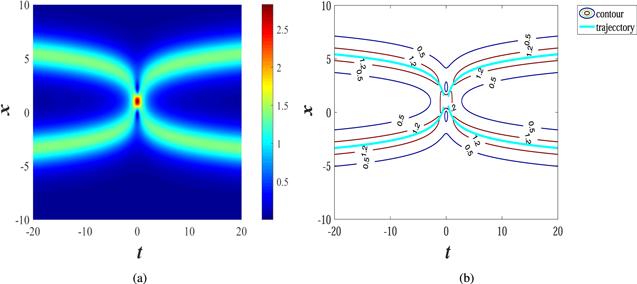
Compared with the tedious Darboux transformation [33, 34], the method of obtaining multiple-pole solutions presented by proposition 2.1 is very fast and simple. In contrast to the mathematically demanding inverse scattering method [23, 31, 32], this method does not require the knowledge of complex analysis to achieve the same results. Figure 1 graphically illustrates that the results obtained in this paper are in high agreement with those obtained by inverse scattering [23, 31, 32] and Darboux transformation [33, 34].
Figure 1. (a) $\left|{u}_{2-p}\right|$ described by equation (4) with parameters $\left\{{k}_{1}=1,\beta =2,{\eta }_{1}^{(0)}=0\right\};$ (b) Contour plot of (a), and the cyan curve is the trajectory of the wave crest predicted by equation (7).
In equation (4), ${\eta }_{1}^{(0)}$ and β jointly determine the position of the double-pole solution at time t = 0. When $\left\{{k}_{1}=a+{\rm{i}}{b},\beta =\pm 2a,{\eta }_{1}^{(0)}=0\right\}$ (a and b are real parameters), the modulus square of a double-pole solution equation (4) can be approximated as two modulus squares of a soliton with varying velocity as ∣t∣ goes to infinity:
The proof process of equation (7) is difficult to write down and perform a rigorous derivation. Even relatively primitive research studies on this subject have only made a few remarks [43] or a passing reference to the process [44]. The approximation described by equation (7) is essentially a planned removal of some relatively low-order terms in $| {u}_{2-p}{| }^{2}$. Equation (7) is correct or incorrect based on whether $| {u}_{2-p}| $ can reach the maximum value $\sqrt{2}| a| $ at infinity only along the trajectories $2{abt}-{ax}\pm$$ \tfrac{\mathrm{ln}\left(16{a}^{4}{t}^{2}\right)}{2}+\tfrac{\mathrm{ln}\left(8{a}^{2}\right)}{2}=0$. The cyan curve in figure 1 (b) represents the two trajectories just mentioned, which intuitively shows that equation (7) is no problem.
in equation (2), then a 4-soliton solution will be reduced to an interaction between two double-pole solutions when $\epsilon \to 0$.
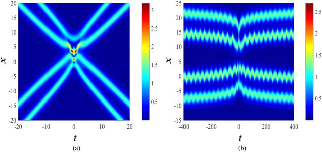
It can be observed from equation (7) that the position of the crest of $\left|{u}_{2-p}\right|$ is jointly determined by the linear term $2{bt}+\tfrac{\mathrm{ln}\left(8{a}^{2}\right)}{2a}$ and the nonlinear term $\pm \tfrac{\mathrm{ln}\left(16{a}^{4}{t}^{2}\right)}{2a}$, among which the linear term plays a major role. Thus, two double-pole solutions will undergo a brief collision shown in figure 2(a) when ${\rm{Im}}\left({k}_{1}\right)\ne {\rm{Im}}\left({k}_{3}\right)$. It is logical that if ${\rm{Im}}\left({k}_{1}\right)={\rm{Im}}\left({k}_{3}\right)$ and the positions of the two double-pole solutions are close enough to each other at the initial moment, then the strong coupling effect is shown in figure 2(b) will occur. In [23], Schiebold also discovered these phenomena in figure 2 through the esoteric and cumbersome operator theoretic approach.
Figure 2. Two different types of interactions between double-pole solutions: (a) a brief collision described by proposition 2.2 with parameters $\left\{{k}_{1}=1+\tfrac{{\rm{i}}}{2},{k}_{3}=1-\tfrac{{\rm{i}}}{2},\beta =2,{\eta }_{1}^{(0)}=0,{\eta }_{3}^{(0)}=0\right\};$ (b) a strong coupling described by proposition 2.2 with parameters $\left\{{k}_{1}=1,{k}_{3}=\tfrac{9}{10},\beta =2,{\eta }_{1}^{(0)}=0,{\eta }_{3}^{(0)}=\tfrac{1}{2}\right\}$.
Unfortunately, continuing to introduce the module resonance condition ${k}_{1}=\pm {k}_{3}^{* }$ would lead to a denominator of 0 for $\exp \left({\theta }_{{jl}}\right)$ in equation (2). This means that in the FNLS system, it is impossible to use two double-pole solutions to generate a degenerate solution of a second-order breather wave through module resonance like the mKdV [42] and complex mKdV [45] equations.
in equation (2), then a 2M-soliton solution will be reduced to an interaction between M double-pole solutions when ε → 0.
Regretfully, the computational difficulty of the N-soliton solution of the FNLS equation is equivalent to that of the 2N-soliton solution of the mKdV equation [42]. Therefore, it is difficult to derive general expressions for the interaction of M double-pole solutions. However, the Darboux transformation method which requires a higher mathematical foundation does not have this defect [43].
in equation (2), then a 3-soliton solution will be reduced to a triple-pole solution ${u}_{3-p}$ when $\epsilon \to 0$, and this triple-pole solution ${u}_{3-p}$ is expressed as
In proposition 3.1, the notations ${\eta }_{1,{k}_{1}}$, ${\eta }_{1,{k}_{1}{k}_{1}}$, ${\eta }_{1,{k}_{1}^{* }}^{* }$ and ${\eta }_{1,{k}_{1}^{* }{k}_{1}^{* }}^{* }$ are defined as follows
respectively. Substituting the constraints equation (10) into (12) and (13), and subsequently, after a very tedious calculation, equation (11) will be obtained when $\epsilon \to 0$. It is easy to see that the proof of proposition 3.1 is very similar to that of proposition 2.1, except that proposition 3.1 involves a bit more computation.□
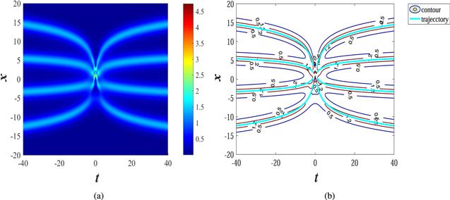
Figure 3 clearly depicts the space-time structure and asymptotic behavior of a triple-pole solution. When $\left\{{k}_{1}=a+{\rm{i}}{b},\beta =\pm 2{a}^{2},{\eta }_{1}^{(0)}=0\right\}$ (a and b are real parameters), the modulus square of a triple-pole solution equation (11) can be approximated as
when ∣t∣ goes to infinity. Equation (14) implies that the extreme value $\sqrt{2}| a| $ of ∣u2−p∣ can be obtained along the trajectories $2{abt}-{ax}\pm \mathrm{ln}\left(8{a}^{4}{t}^{2}\right)+\tfrac{\mathrm{ln}\left(8{a}^{2}\right)}{2}=0$ and $2{abt}-{ax}+\tfrac{\mathrm{ln}\left(8{a}^{2}\right)}{2}=0$. The cyan curve in figure 3(b) visually verifies the correctness of equation (14).
Figure 3. (a) $\left|{u}_{3-p}\right|$ described by equation (11) with parameters $\left\{{k}_{1}=1,\beta =2,{\eta }_{1}^{(0)}=0\right\};$ (b) Contour plot of (a), and the cyan curve represents the trajectory predicted by equation (14).
in equation (2), then the N-soliton solution will be reduced to a mutiple-pole solution ${u}_{N-p}$ when $\epsilon \to 0$.
Here ${C}_{n}^{r},\left(0\leqslant r\leqslant n,r,n\in {\mathbb{N}}\right)$ implies binomial coefficients, and ${C}_{n}^{r}=\tfrac{n!}{r!(n-r)!}$.
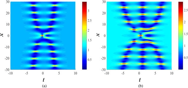
If N = 4, then proposition 3.2 will represent a quadruple-pole solution as shown in figure 4. When ∣t∣ goes to infinity, the quadruple-pole depicted in figure 4 has the following asymptotic behavior:
The cyan curves in figure 4(b) represent the four trajectories $\{-x\pm \tfrac{\mathrm{ln}\left(4{t}^{2}\right)}{2}+\tfrac{3\mathrm{ln}\left(2\right)}{2}=0$, $-x\pm \tfrac{3}{2}\mathrm{ln}\left(\tfrac{8}{3}\sqrt[3]{6}{t}^{2}\right)+\tfrac{3\mathrm{ln}\left(2\right)}{2}=0\}$ along which the extreme points of ∣${u}_{4-p}$∣ can be reached. Unfortunately, the general expression for the quadruple-pole solution is so lengthy that its asymptotic behavior is difficult to find.
Figure 4. (a) $\left|{u}_{4-p}\right|$ described by proposition 3.2 with parameters $\left\{N=4,{k}_{1}=1,\beta =\tfrac{4}{3},{\eta }_{1}^{(0)}=0\right\}$; (b) Contour plot of (a), and the cyan curve represents the trajectory predicted by equation (16).
4. Degeneration of N-breather solutions
The method of deriving multiple-pole solutions directly from N-soliton solutions described in the previous two sections is also applicable to finding degenerate solutions of higher-order breather waves. With reference to [21], the N-breather solution of the FNLS equation takes the following form:
in equation (17), then a 2-breather solution will be reduced to a degenerate solution ${u}_{2-{db}}$ when $\epsilon \to 0$, and this degenerate solution of a 2-breather solution is expressed as
The expression of equation (19) is verbose, so it is necessary to assign values to the parameters so that readers can easily observe the algebraic structure of u2−db and verify proposition 4.1. By selecting parameters $\left\{k=0,{\rho }_{0}=1,{\phi }_{1}=\tfrac{\pi }{4},\beta =1,{\omega }_{1}^{(0)}=0\right\}$, equation (19) can be simplified to
Figure 5. (a) A degenerate solution of a 2-breather solution $\left|{u}_{2-{db}}\right|$ described by equation (20); (b) by selecting parameters $\left\{k=0,{\rho }_{0}=1,{\phi }_{1}=\tfrac{\pi }{4},\beta =1,{\omega }_{1}^{(0)}=0,N=3\right\}$ in proposition 4.2, a special degenerate solution ∣u3−db∣ can be derived from a 3-breather solution.
Wang et al obtained degenerate solutions of breather solutions by Darboux transformation and pointed out how degenerate solutions of breather solutions reduce into higher-order rogue waves for the first time [29]. However, on the basis of the bilinear method, only a breather wave can be reduced to a first-order rogue wave by means of the long wave limit [21]. To put it bluntly, equation (17) degenerates into a first-order rogue wave by setting {N = 1, φ1 = φ1ε, φ2 = ${\varphi }_{1}^{* }\epsilon +\pi ,{{\rm{\Omega }}}_{1}^{(0)}$ = ${\rm{i}}\pi ,{{\rm{\Omega }}}_{2}^{(0)}$ = −iπ, ε → 0}. Regretfully, there are no relevant studies showing that the long-wave limit method can derive a higher-order rogue wave solution from a N-breather solution.
The mechanism for generating higher-order rogue waves consists of two steps: (i) obtaining a degenerate solution of a N-breather solution; (ii) making the period of the degenerate solution generated in the first step to infinity [29]. These two steps are also the main problems encountered in obtaining higher-order rogue wave solutions using bilinear methods. This study solves the first important step, which makes the idea of deriving higher-order waves from breather waves using bilinear methods a big step closer to becoming a reality. For obtaining a higher-order degenerate solution of a N-breather solution, we have the following proposition:
in equation (17), then a N-breather solution will be reduced to a Nth-order degenerate solution ${u}_{N-{db}}$ when $\epsilon \to 0$.
Here ${C}_{n}^{r},\left(0\leqslant r\leqslant n,r,n\in {\mathbb{N}}\right)$ implies binomial coefficients, and ${C}_{n}^{r}=\tfrac{n!}{r!(n-r)!}$.
5. Conclusion
Based on the bilinear method, this paper systematically investigates the multiple-pole solutions and degenerate solutions of focusing nonlinear Schrödinger equation by some skillful limiting means. The greatest innovation of this study is that it provides a simple and fast method to derive the multiple-pole solutions of FNLS equation. Proposition 2.1 and proposition 3.1 give specific approaches to the double-pole solution and the triple-pole solution and give general expressions equation (4) and equation (11) for the relevant solutions. Proposition 3.2 summarizes proposition 2.1 and proposition 3.1, and points out a general method to derive multiple-pole solutions directly from N-soliton solutions. The space-time structure and dynamical properties of these multi-pole solutions are described by beautiful images (figures 1, 3, 4) and rigorous mathematical expressions (equations (7), (14), (16)) respectively. Similarly, this limit method mentioned in this paper can also be used to achieve degeneration of a N-breather solution (see proposition 4.1 and proposition 4.2 for details). There are two limiting steps to convert the higher-order breather solution to the higher-order rogue wave solution. For the first limiting step, proposition 4.1 has been able to derive a degenerate solution from the N-breather solution; however, for the second step, it is worth further thinking how to convert the higher-order degenerate solution obtained at the first stage into a higher-order rogue wave. In addition, this method can be extended to a derivative Schrödinger equation, sine-Gorden equation, mKdV equation and so on.
Declarations
Conflict of interest
The authors declare that they have no conflict of interests.
This research is supported by the Natural Science Foundation of Guangdong Province of China (No. 2021A1515012214), the Science and Technology Program of Guangzhou (No. 2 019 050 001), National Natural Science Foundation of China (Nos. 12 175 111), and K C Wong Magna Fund in Ningbo University. The authors sincerely thank Dr Jiguang Rao (Shenzhen University) for his suggestions and encouragement.
AkinyemiL2021 Novel approach to the analysis of fifth-order weakly nonlocal fractional Schrödinger equation with Caputo derivative Results Phys.31 104958
MartinezH YKhaterM M ARezazadehHIncM2021 Analytical novel solutions to the fractional optical dynamics in a medium with polynomial law nonlinearity and higher order dispersion with a new local fractional derivative Phys. Lett. A420 127744
LiJ HChenQ QLiB2021 Resonance Y-type soliton solutions and some new types of hybrid solutions in the (2+1)-dimensional Sawada-Kotera equation Commun. Theor. Phys.73 045006
LiJ HLiB2021 Solving forward and inverse problems of the nonlinear Schrödinger equation with the generalized PT -symmetric Scarf-II potential via PINN deep learning Commun. Theor. Phys.73 125001
FanRZhangZLiB2020 Multisoliton solutions with even numbers and its generated solutions for nonlocal Fokas-Lenells equation Commun. Theor. Phys.72 125007
AblowitzM JClarksonP A1991Solitons, Nonlinear Evolution Equations and Inverse Scattering Cambridge Cambridge University Press
19
HirotaR1976 Direct method of finding exact solutions of nonlinear evolution equations Bäcklund Transformations Lect. Notes. Math. MiuraR Mvol 515 New York Springer 40
20
AktosunTDemontisFMeeC2007 Exact solutions to the focusing nonlinear Schrödinger equation Inverse Problems23 2171
FengB FLingL MTakahashiD A2020 Multi-breathers and high order rogue waves for the nonlinear Schrödinger equation on the elliptic function background Stud. Appl. Math.144 46
ZakharovVShabatA1970 Exact theory of two-dimensional self-focusing and one-dimensional self-modulation of waves in nonlinear media J. Exp. Theor. Phys.34 62
33
BilmanDBuckinghamR2019 Large-order asymptotics for multiple-pole solitons of the focusing nonlinear schrödinger equation J. Nonlinear Sci.29 2185
LiuJ GOsmanM S2021 Nonlinear dynamics for different nonautonomous wave structures solutions of a 3D variable-coefficient generalized shallow water wave equation Chin. J. Phys.
LiuJ GZhuW HOsmanM SMaW X2020 An explicit plethora of different classes of interactive lump solutions for an extension form of 3D-Jimbo-Miwa model Eur. Phys. J. Plus135 412
LiuJ G2020 The general bilinear techniques for studying the propagation of mixed-type periodic and lump-type solutions in a homogenous-dispersive medium AIP Adv.10 105325
OsmanM S2020 Different wave structures and stability analysis for the generalized (2+1)- dimensional Camassa–Holm–Kadomtsev–Petviashvili equation Phys. Scr.95 035229


