


1. Introduction
In recent decades, integrable systems have attracted extensive attention in describing nonlinear phenomena in various areas, such as fluid mechanics, nonlinear optics, Bose–Einstein condensates, plasma physics and other fields [1, 2]. A crucial feature of an integrable system is that it can be expressed as a compatibility condition of two linear spectral problems, i.e. a Lax pair, which enables researchers to investigate it via the inverse scattering method [1], Darboux transformation [3–6], algebra-geometric method [7–9], Riemann–Hilbert approach [10–15], etc. The Riemann–Hilbert approach is an effective tool for solving the integrable models and studying their long-time asymptotics and other properties.
In this paper, we will use the Riemann–Hilbert approach to investigate the following AB system
$\begin{eqnarray}{A}_{{xt}}={AB},\quad {B}_{x}=-\displaystyle \frac{1}{2}{\left(| A{| }^{2}\right)}_{t},\end{eqnarray}$
with a normalization condition $\begin{eqnarray}| {A}_{t}{| }^{2}+{B}^{2}=1,\end{eqnarray}$
where A = A(x, t) is a complex function and B = B(x, t) is a real function [16]. The AB system, first proposed by Pedlosky using the singular perturbation theory [17], is a significant integrable model since it can describe unstable baroclinic wave packets in geophysical fluids and the propagation of mesoscale gravity flow in nonlinear optics [18–21]. Moreover, the AB system can be reduced to the sine-Gordon equation for real A or the self-induced transparency equations for complex A [22]. Rogue wave solutions, breathers and N-soliton solutions for the AB system have been derived by resorting to the Darboux transformation [23, 24] and the dressing method [25]. Multi-dark-dark solitons and multi-bright-bright solitons have been found for repulsive AB system via determinants [26, 27]. Recently, long-time asymptotics of solutions for the AB system with initial value problems have been studied through the nonlinear steepest-decent method [28]. For ultra-short optical pulse propagation models such as the short pulse equation, the associated Riemann–Hilbert problem and explicit soliton formulae may help to better understand the propagation mechanism and characteristics [29, 30]. Therefore, the present paper is devoted to exploring the AB system by utilizing the Riemann–Hilbert approach, from which explicit multi-bright-dark soliton solutions in the reflectionless case are obtained with potential functions A decaying to zero and B decaying to 1 at sufficiently fast rates as x → ∞ . In particular, we find that the multi-soliton collisions are elastic.The arrangement of this paper is as follows. In section 2 , we construct the sectional analytic function and establish the Riemann–Hilbert problem on the basis of the spectral analysis. With the aid of symmetry relations, we solve the non-regular matrix Riemann–Hilbert problem. Section 3 focuses on the time evolution of scattering data and the reconstruction of potentials. In section 4 , we obtain explicit N-soliton solutions to the AB system in the reflectionless case. In particular, we find that the soliton collisions are elastic. The last section contains some discussions.
2. Riemann–Hilbert problem
The AB system (1.1 ) is related to the following Lax pair, namely, two 2 × 2 matrix spectral problems [16]2.1 ) gives zero-curature equation, Ut − Vx + [U, V] = 0, which is equivalent to the AB system (1.1 ). We assume that potential function A decays to zero and B decays to 1 at sufficiently fast rates as x → ± ∞ , which implies that matrix solution $\Psi$ of (2.1 ) has an asymptotic expression ${{\rm{e}}}^{-{\rm{i}}\lambda {\sigma }_{3}x-\tfrac{1}{4{\rm{i}}\lambda }{\sigma }_{3}t}.$ For convenience, we introduce a new matrix spectral function J = J(x, t, λ) as follows2.1 ) can be rewritten in the following equivalent form
$\begin{eqnarray}{{\rm{\Psi }}}_{x}=U{\rm{\Psi }}=(-{\rm{i}}\lambda {\sigma }_{3}+\widetilde{U}){\rm{\Psi }},\end{eqnarray}$
$\begin{eqnarray}{{\rm{\Psi }}}_{t}=V{\rm{\Psi }}=\displaystyle \frac{1}{4{\rm{i}}\lambda }(-B{\sigma }_{3}+\widetilde{V}){\rm{\Psi }},\end{eqnarray}$
where $\Psi$ = $\Psi$(x, t, λ) is a matrix-valued function, λ is a constant spectral parameter and $\widetilde{U},\widetilde{V},{\sigma }_{3}$ are defined as follows $\begin{eqnarray*}\widetilde{U}=\left(\begin{array}{cc}0 & \displaystyle \frac{1}{2}A\\ -\displaystyle \frac{1}{2}{A}^{* } & 0\end{array}\right),\quad \widetilde{V}=\left(\begin{array}{cc}0 & {A}_{t}\\ {A}_{t}^{* } & 0\end{array}\right),\quad {\sigma }_{3}=\left(\begin{array}{cc}1 & 0\\ 0 & -1\end{array}\right).\end{eqnarray*}$
The compatibility condition of ( $\begin{eqnarray}J={\rm{\Psi }}{E}^{-1},\end{eqnarray}$
where $E={{\rm{e}}}^{-{\rm{i}}\lambda {\sigma }_{3}x-\tfrac{1}{4{\rm{i}}\lambda }{\sigma }_{3}t}$. Through direct calculation, we can see that the Lax pair ( $\begin{eqnarray}{J}_{x}={\rm{i}}\lambda J{\sigma }_{3}+{UJ}={\rm{i}}\lambda J{\sigma }_{3}-{\rm{i}}\lambda {\sigma }_{3}J+\widetilde{U}J,\end{eqnarray}$
$\begin{eqnarray}{J}_{t}=\displaystyle \frac{1}{4{\rm{i}}\lambda }J{\sigma }_{3}+{VJ}=\displaystyle \frac{1}{4{\rm{i}}\lambda }(J{\sigma }_{3}-B{\sigma }_{3}J+\widetilde{V}J).\end{eqnarray}$
In the following, we will carry out spectral analysis, for which we construct the matrix Jost solutions J± = J±(x, λ) of the (2.3a ) with the asymptotic condition2.1 ), they must be linearly dependent, so there exists a scattering matrix S(λ) such that2.2 ) and (2.8 ). Combining with equation (2.9 ), we find $\det S(\lambda )=1$. In order to obtain a Riemann–Hilbert problem for the AB system, we define a new matrix function P+ = P+(x, λ):2.3a ) and is analytic for λ ∈ D+ with the following asymptotic condition2.3a )
$\begin{eqnarray}{J}_{\pm }(x,\lambda )\to I,\quad x\to \pm \infty ,\end{eqnarray}$
where I is the 2 × 2 identity matrix. It is easy to verify that J± are uniquely determined by the Volterra integral equations $\begin{eqnarray}{J}_{+}(x,\lambda )=I-{\int }_{x}^{+\infty }{{\rm{e}}}^{{\rm{i}}\lambda {\sigma }_{3}(y-x)}\widetilde{U}(y){J}_{+}(y,\lambda ){{\rm{e}}}^{-{\rm{i}}\lambda {\sigma }_{3}(y-x)}{\rm{d}}y,\end{eqnarray}$
$\begin{eqnarray}{J}_{-}(x,\lambda )=I+{\int }_{-\infty }^{x}{{\rm{e}}}^{{\rm{i}}\lambda {\sigma }_{3}(y-x)}\widetilde{U}(y){J}_{-}(y,\lambda ){{\rm{e}}}^{-{\rm{i}}\lambda {\sigma }_{3}(y-x)}{\rm{d}}y.\end{eqnarray}$
The Jost solutions can be divided into columns $\begin{eqnarray}{J}_{\pm }=({\left[{J}_{\pm }\right]}_{1},{\left[{J}_{\pm }\right]}_{2}),\end{eqnarray}$
where ${\left[{J}_{\pm }\right]}_{l},(l=1,2),$ is the lth column of J±. Hence, the convergence of the above Volterra integral equations implies that J± allows analytical continuation off the real axis $\lambda \in {\mathbb{R}}$. It is not difficult to find that ${\left[{J}_{-}\right]}_{1}$ and ${\left[{J}_{+}\right]}_{2}$ can be analytically extended to the upper half-plane D+, and ${\left[{J}_{+}\right]}_{1}$ ang ${\left[{J}_{-}\right]}_{2}$ to the lower half-plane D− with $\begin{eqnarray}\begin{array}{rcl}{D}_{+} & = & \left\{\lambda \in C| \arg \lambda \in (0,\pi )\right\},\\ {D}_{-} & = & \left\{\lambda \in C| \arg \lambda \in (\pi ,2\pi )\right\}.\end{array}\end{eqnarray}$
It is easy to see that $\begin{eqnarray}{{\rm{\Psi }}}_{\pm }(x,\lambda )={J}_{\pm }{E}_{1},\quad {E}_{1}={{\rm{e}}}^{-{\rm{i}}\lambda {\sigma }_{3}x}\end{eqnarray}$
are the fundamental solution matrixes of ( $\begin{eqnarray}{{\rm{\Psi }}}_{-}(x,\lambda )={{\rm{\Psi }}}_{+}(x,\lambda )S(\lambda ),\quad \lambda \in {\mathbb{R}},\end{eqnarray}$
where $S(\lambda )={\left({s}_{{ij}}\right)}_{2\times 2}$. By considering the formulas ${\left(\det {{\rm{\Psi }}}_{\pm }\right)}_{x}=\det {{\rm{\Psi }}}_{\pm }\mathrm{tr}({\left({{\rm{\Psi }}}_{\pm }\right)}_{x}{{\rm{\Psi }}}_{\pm }^{-1})$ and $\mathrm{tr}(U)=0$, we arrive at ${\left(\det {{\rm{\Psi }}}_{\pm }\right)}_{x}=0$, which implies that $\det {{\rm{\Psi }}}_{\pm }(x,\lambda )$ are independent of x. We can also obtain $\det {J}_{\pm }(x,\lambda )=1$ from ( $\begin{eqnarray}{P}^{+}=({\left[{J}_{-}\right]}_{1},{\left[{J}_{+}\right]}_{2})={J}_{+}({E}_{1}{{SE}}_{1}^{-1}{H}_{1}+{H}_{2}),\end{eqnarray}$
where H1 = diag(1, 0), H2 = diag(0, 1). Based on the analytic properties of ${\left[{J}_{\pm }\right]}_{l}\quad (l=1,2)$, we can see that P+ satisfies ( $\begin{eqnarray}{P}^{+}(x,\lambda )\to I,\quad \lambda \in {D}_{+}\to \infty .\end{eqnarray}$
Similarly, we introduce that a matrix function P− = P−(x, λ) is analytic for λ ∈ D−. Consider the inverse matrix of J± satisfying the following adjoint equation of ( $\begin{eqnarray}{K}_{x}=-{\rm{i}}\lambda {\sigma }_{3}K-{KU},\end{eqnarray}$
which can be written as $\begin{eqnarray}{J}_{\pm }^{-1}=\left(\begin{array}{c}{\left[{J}_{\pm }^{-1}\right]}^{1}\\ {\left[{J}_{\pm }^{-1}\right]}^{2}\end{array}\right).\end{eqnarray}$
It is easy to calculate that ${\left[{J}_{+}^{-1}\right]}^{1},{\left[{J}_{-}^{-1}\right]}^{2}$ can be analytically extended to the upper half-plane D+ and ${\left[{J}_{+}^{-1}\right]}^{2},{\left[{J}_{-}^{-1}\right]}^{1}$ to the lower half-plane D−. Let us define the matrix function $\begin{eqnarray}{P}^{-}=\left(\begin{array}{c}{\left[{J}_{-}^{-1}\right]}^{1}\\ {\left[{J}_{+}^{-1}\right]}^{2}\end{array}\right)=({H}_{1}{E}_{1}{{RE}}_{1}^{-1}+{H}_{2}){J}_{+}^{-1},\end{eqnarray}$
where $R(\lambda )={{\rm{\Psi }}}_{-}^{-1}{{\rm{\Psi }}}_{+}={S}^{-1}(\lambda )={\left({r}_{{ij}}\right)}_{2\,\times \,2}$. In addition, by considering the asymptotic behavior of P− at large λ ∈ D−, we find that $\begin{eqnarray}{P}^{-}(x,\lambda )\to I,\quad \lambda \to \infty .\end{eqnarray}$
Note that two matrix functions P+ and P− are analytic in D+ and D−, respectively. On the real line, they have the following relationship2.16 ) is the Riemann–Hilbert problem on the real axis for the AB system with an associated canonical condition2.10 ) and (2.14 ), we arrive at
$\begin{eqnarray}{P}^{-}(x,\lambda ){P}^{+}(x,\lambda )=G(x,\lambda ),\quad \lambda \in {\mathbb{R}},\end{eqnarray}$
where $\begin{eqnarray}G(x,\lambda )=\left(\begin{array}{cc}1 & {r}_{12}(\lambda ){{\rm{e}}}^{-2{\rm{i}}\lambda x}\\ {s}_{21}(\lambda ){{\rm{e}}}^{2{\rm{i}}\lambda x} & 1\end{array}\right).\end{eqnarray}$
Equation ( $\begin{eqnarray}{P}^{\pm }\to I,\quad \lambda \to \infty .\end{eqnarray}$
In the subsequent text, we will discuss how to solve the regular and non-regular Riemann–Hilbert problem. From the relations ( $\begin{eqnarray}\det {P}^{+}={s}_{11}(\lambda ),\quad \det {P}^{-}={r}_{11}(\lambda ).\end{eqnarray}$
First, let us consider the regular Riemann–Hilbert problem, i.e. $\det {P}^{+}\ne 0$ in D+ and $\det {P}^{-}\ne 0$ in D−, respectively. Formula (2.16 ) can be rewritten in the following form2.16 ) satisfying the canonical condition (2.18 ):2.2 ), we obtain2.8 ) and (2.9 ), one infers2.26 ) and (2.19 ), we find that if λj is a zero of $\det {P}^{+}(\lambda )$, then ${\hat{\lambda }}_{j}={\lambda }_{j}^{* }$ is a zero of $\det {P}^{-}(\lambda )$ . Assume that $\det {P}^{+}(\lambda )$ has N simple zeros ${\{{\lambda }_{j}\}}_{1}^{N}$, it is easy to see that the kernels of P+(λj) and ${P}^{-}({\hat{\lambda }}_{j})$ contain only a single column vector νj and row vector ${\hat{\nu }}_{j}$, respectively, that is2.27a ), we obtain2.26 ), we have2.27b ) and (2.29 ) imply that2.16 ) with the canonical condition (2.18 ) by the following theorem.
$\begin{eqnarray}{\left({P}^{+}\right)}^{-1}(\lambda )-{P}^{-}(\lambda )=\hat{G}(\lambda ){\left({P}^{+}\right)}^{-1}(\lambda ),\quad \lambda \in {\mathbb{R}},\end{eqnarray}$
where $\begin{eqnarray*}\hat{G}(\lambda )=I-G(\lambda ).\end{eqnarray*}$
Then using the Plemelj formula, we can obtain the solution of ( $\begin{eqnarray}{\left({P}^{+}\right)}^{-1}(\lambda )=I+\displaystyle \frac{1}{2\pi {\rm{i}}}{\int }_{-\infty }^{+\infty }\displaystyle \frac{\hat{G}(\xi ){\left({P}^{+}\right)}^{-1}(\xi )}{\xi -\lambda }{\rm{d}}\xi ,\quad \lambda \in {D}_{+}.\end{eqnarray}$
Next, we will consider the non-regular Riemann–Hilbert problem based on the symmetry relations. Assume $\det {P}^{+}$ and $\det {P}^{-}$ have simple zeros in D+ and D−, respectively. It is easy to see that the matrixes U(λ) and V(λ) satisfy the symmetry relations $\begin{eqnarray}\begin{array}{l}{U}^{\dagger }({\lambda }^{* })=-U(\lambda ),\\ {V}^{\dagger }({\lambda }^{* })=-V(\lambda ),\end{array}\end{eqnarray}$
where the superscript † is the Hermitian conjugate. We can easily verify that $\Psi$† (λ*) and $\Psi$−1(λ) satisfy the same differential equation and boundary condition. Therefore, by the uniqueness of the solution, we arrive at $\begin{eqnarray}{{\rm{\Psi }}}^{\dagger }({\lambda }^{* })={{\rm{\Psi }}}^{-1}(\lambda ).\end{eqnarray}$
From ( $\begin{eqnarray}{J}^{\dagger }({\lambda }^{* })={J}^{-1}(\lambda ).\end{eqnarray}$
Using the relations ( $\begin{eqnarray}{S}^{\dagger }({\lambda }^{* })=R(\lambda ),\end{eqnarray}$
which implies that $\overline{{s}_{11}}({\lambda }^{* })={r}_{11}(\lambda )$. Furthermore, from the definitions of P+ and P−, we can deduce the following relation $\begin{eqnarray}{\left({P}^{+}\right)}^{\dagger }({\lambda }^{* })={P}^{-}(\lambda ).\end{eqnarray}$
According to symmetric relations ( $\begin{eqnarray}{P}^{+}({\lambda }_{j}){\nu }_{j}=0,\ 1\leqslant j\leqslant N,\end{eqnarray}$
$\begin{eqnarray}{\hat{\nu }}_{j}{P}^{-}({\hat{\lambda }}_{j})=0,\ 1\leqslant j\leqslant N.\end{eqnarray}$
If we take the Hermitian conjugate of ( $\begin{eqnarray}{\nu }_{j}^{\dagger }{\left({P}^{+}\right)}^{\dagger }({\lambda }_{j})=0,\quad 1\leqslant j\leqslant N.\end{eqnarray}$
According to ( $\begin{eqnarray}{\nu }_{j}^{\dagger }{P}^{-}({\lambda }_{j}^{* })=0,\quad 1\leqslant j\leqslant N.\end{eqnarray}$
Equations ( $\begin{eqnarray}{\hat{\nu }}_{j}={\nu }_{j}^{\dagger }.\end{eqnarray}$
Based on the above analysis, we could solve the non-regular matrix Riemann–Hilbert problem ( The solution of the non-regular matrix Riemann–Hilbert problem (
$\begin{eqnarray}{P}^{+}(\lambda )={\hat{P}}^{+}(\lambda ){\rm{\Gamma }}(\lambda ),\end{eqnarray}$
$\begin{eqnarray}{P}^{-}(\lambda )={{\rm{\Gamma }}}^{-1}(\lambda ){\hat{P}}^{-}(\lambda ),\end{eqnarray}$
where $\begin{eqnarray}{\rm{\Gamma }}(\lambda )=I+\sum _{i,j=1}^{N}\displaystyle \frac{{\nu }_{i}{\hat{\nu }}_{j}{\left({M}^{-1}\right)}_{{ij}}}{\lambda -\hat{{\lambda }_{j}}},\end{eqnarray}$
$\begin{eqnarray}{{\rm{\Gamma }}}^{-1}(\lambda )=I-\sum _{i,j=1}^{N}\displaystyle \frac{{\nu }_{i}{\hat{\nu }}_{j}{\left({M}^{-1}\right)}_{{ij}}}{\lambda -{\lambda }_{i}},\end{eqnarray}$
and $M=({M}_{{ij}})$ is an N × N matrix, $\begin{eqnarray}{M}_{{ij}}=\displaystyle \frac{{\hat{\nu }}_{i}{\nu }_{j}}{{\hat{\lambda }}_{i}-{\lambda }_{j}},\quad 1\leqslant i,j\leqslant N,\end{eqnarray}$
$\begin{eqnarray}\det {\rm{\Gamma }}(\lambda )=\prod _{j=1}^{N}\displaystyle \frac{\lambda -{\lambda }_{j}}{\lambda -{\hat{\lambda }}_{j}}.\end{eqnarray}$
Matrix function ${\hat{P}}^{\pm }(\lambda )$ is the unique solution to the following regular Riemann–Hilbert problem $\begin{eqnarray}{\hat{P}}^{-}(\lambda ){\hat{P}}^{+}(\lambda )={\rm{\Gamma }}(\lambda )G(\lambda ){{\rm{\Gamma }}}^{-1}(\lambda ),\quad \lambda \in {\mathbb{R}},\end{eqnarray}$
where ${\hat{P}}^{\pm }$ are analytic in ${D}_{\pm }$ and $\begin{eqnarray}{\hat{P}}^{\pm }(\lambda )\to I,\quad \lambda \in {D}_{\pm }\to \infty .\end{eqnarray}$
3. Reconstruction of potentials
In this section, we shall establish the time evolution of the scattering data and reconstruct the potentials A and B. From the solutions of the non-regular Riemann–Hilbert problem (2.16 ) as given in theorem 2.1, we find that the scattering data needed to solve this non-regular Riemann–Hilbert problem is
$\begin{eqnarray}\{{s}_{21}(\lambda ),{r}_{12}(\lambda ),\lambda \in {\mathbb{R}};{\lambda }_{j},{\hat{\lambda }}_{j},{\nu }_{j},{\hat{\nu }}_{j},1\leqslant j\leqslant N\}.\end{eqnarray}$
This is called the minimal scattering data. In these scattering data, the vectors νj and ${\hat{\nu }}_{j}$ are related to x, while the other vectors are not related to x.Our starting point is equation (2.27 ) for νj and ${\hat{\nu }}_{j}$. Taking the derivative of equation (2.3a ) with respect to x, we arrive at2.3b ) with respect to t yields3.4 ) and (3.6 ), we obtain
$\begin{eqnarray}{P}_{x}^{+}({\lambda }_{j},x,t){\nu }_{j}+{P}^{+}({\lambda }_{j},x,t)\displaystyle \frac{{\rm{d}}{\nu }_{j}}{{\rm{d}}x}=0,\end{eqnarray}$
and $\begin{eqnarray}{P}_{x}^{+}({\lambda }_{j},x,t)={\rm{i}}{\lambda }_{j}{P}^{+}({\lambda }_{j},x,t){\sigma }_{3}+{{UP}}^{+}({\lambda }_{j},x,t).\end{eqnarray}$
Thus, we have $\begin{eqnarray}{\rm{i}}{\lambda }_{j}{\sigma }_{3}{\nu }_{j}+\displaystyle \frac{{\rm{d}}{\nu }_{j}}{{\rm{d}}x}=0.\end{eqnarray}$
Similarly, taking the derivative of equation ( $\begin{eqnarray}\begin{array}{l}{P}_{t}^{+}({\lambda }_{j},x,t){\nu }_{j}+{P}^{+}({\lambda }_{j},x,t)\displaystyle \frac{{\rm{d}}{\nu }_{j}}{{\rm{d}}t}=0,\\ {P}_{t}^{+}({\lambda }_{j},x,t)=\displaystyle \frac{1}{4{\rm{i}}{\lambda }_{j}}{P}^{+}({\lambda }_{j},x,t){\sigma }_{3}+{{VP}}^{+}({\lambda }_{j},x,t),\end{array}\end{eqnarray}$
which implies $\begin{eqnarray}\displaystyle \frac{1}{4{\rm{i}}{\lambda }_{j}}{\sigma }_{3}{\nu }_{j}+\displaystyle \frac{{\rm{d}}{\nu }_{j}}{{\rm{d}}t}=0.\end{eqnarray}$
By considering ( $\begin{eqnarray}{\nu }_{j}={{\rm{e}}}^{-{\rm{i}}{\lambda }_{j}{\sigma }_{3}x-\displaystyle \frac{1}{4{\rm{i}}{\lambda }_{j}}{\sigma }_{3}t}{\nu }_{j}^{0},\end{eqnarray}$
where ${\nu }_{j}^{0}$ is a constant. A similar calculation for ${\hat{\nu }}_{j}$ deduces $\begin{eqnarray}{\hat{\nu }}_{j}={\nu }_{j}^{1}{{\rm{e}}}^{{\rm{i}}{\lambda }_{j}^{\ast }{\sigma }_{3}x+\displaystyle \frac{1}{4{\rm{i}}{\lambda }_{j}^{\ast }}{\sigma }_{3}t},\end{eqnarray}$
where ${\nu }_{j}^{1}$ is the Hermitian conjugate of ${\nu }_{j}^{0}$.Since the matrix function J± satisfies the spectral equation (2.3b ), we get3.9 ) by the matrix ${E}_{1}={{\rm{e}}}^{-{\rm{i}}\lambda {\sigma }_{3}x}$, we arrive at2.9 ) for the scattering matrix can be rewritten as2.3b ), that is3.13 ) and (3.14 ), we deduce2.16 ) can be solved from the given scattering data (s21, r12), then the potentials A and B can be reconstructed from the asymptotic expansion of P+ at large λ. In fact, since P+ is a solution of the scattering problem (2.3a ) and its adjoint problem (2.12 ), respectively, we expand P+ at large λ as3.17 ) into (2.3 ) and collecting terms of the same power in λ, we can derive the following expressions2.37 ) can be solved by the Plemelj formula and expressed as an integral equation:2.33 ), we arrive at2.31 ), (3.22 ) and (3.23 ), we obtain from ${\left({P}^{+}\right)}^{(1)}$ in the expansion (3.17 ) of P+ that
$\begin{eqnarray}{\left({J}_{\pm }\right)}_{t}=\displaystyle \frac{1}{4{\rm{i}}\lambda }({J}_{\pm }{\sigma }_{3}-B{\sigma }_{3}{J}_{\pm }+\widetilde{V}{J}_{\pm }).\end{eqnarray}$
Multiplying ( $\begin{eqnarray}{\left({J}_{\pm }{E}_{1}\right)}_{t}=\displaystyle \frac{1}{4{\rm{i}}\lambda }({J}_{\pm }{E}_{1}{\sigma }_{3}-B{\sigma }_{3}{J}_{\pm }{E}_{1}+\widetilde{V}{J}_{\pm }{E}_{1}).\end{eqnarray}$
The definition ( $\begin{eqnarray}{J}_{-}{E}_{1}={J}_{+}{E}_{1}S,\lambda \in {\mathbb{R}},\end{eqnarray}$
from which we see that J+E1S also satisfies the same temporal equation ( $\begin{eqnarray}{\left({J}_{+}{E}_{1}S\right)}_{t}=\displaystyle \frac{1}{4{\rm{i}}\lambda }({J}_{+}{E}_{1}S{\sigma }_{3}-B{\sigma }_{3}{J}_{+}{E}_{1}S+\widetilde{V}{J}_{+}{E}_{1}S).\end{eqnarray}$
Taking the limit x → ∞ and combining the boundary conditions satisfied by A and B, we have: $\begin{eqnarray}{S}_{t}=\displaystyle \frac{-1}{4{\rm{i}}\lambda }[{\sigma }_{3},S],\end{eqnarray}$
where [σ3, S] = σ3S − Sσ3 is the commutator. In a similar way, we obtain $\begin{eqnarray}{R}_{t}=\displaystyle \frac{-1}{4{\rm{i}}\lambda }[{\sigma }_{3},R].\end{eqnarray}$
According to equations ( $\begin{eqnarray}\displaystyle \frac{\partial {s}_{21}}{\partial t}=\displaystyle \frac{1}{2{\rm{i}}\lambda }{s}_{21},\quad \displaystyle \frac{\partial {r}_{12}}{\partial t}=\displaystyle \frac{-1}{2{\rm{i}}\lambda }{r}_{12},\quad \displaystyle \frac{\partial {s}_{11}}{\partial t}=\displaystyle \frac{\partial {r}_{11}}{\partial t}=0.\end{eqnarray}$
Thus $\begin{eqnarray}{s}_{21}(t;\lambda )={s}_{21}(0;\lambda ){{\rm{e}}}^{\tfrac{1}{2{\rm{i}}\lambda }t},\quad {r}_{12}(t;\lambda )={r}_{12}(0;\lambda ){{\rm{e}}}^{\tfrac{-1}{2{\rm{i}}\lambda }t}.\end{eqnarray}$
If the Riemann–Hilbert problem ( $\begin{eqnarray}{P}^{+}=I+{\lambda }^{-1}{\left({P}^{+}\right)}^{(1)}+{\lambda }^{-2}{\left({P}^{+}\right)}^{(2)}+{\lambda }^{-3}{\left({P}^{+}\right)}^{(3)}+.....,\,\lambda \to \infty .\end{eqnarray}$
Then by substituting ( $\begin{eqnarray}\begin{array}{rcl}A & = & 4{\rm{i}}{\left({\left({P}^{+}\right)}^{(1)}\right)}_{12},\\ B & = & 1-4{\rm{i}}{\left({\left({P}^{+}\right)}_{t}^{(1)}\right)}_{11}=1+4{\rm{i}}{\left({\left({P}^{+}\right)}_{t}^{(1)}\right)}_{22}.\end{array}\end{eqnarray}$
According to theorem 2.1, the solution to equation ( $\begin{eqnarray}\begin{array}{l}{\left({\hat{P}}^{+}\right)}^{-1}(\lambda )=I+\displaystyle \frac{1}{2\pi {\rm{i}}}\\ \times {\displaystyle \int }_{-\infty }^{+\infty }\displaystyle \frac{{\rm{\Gamma }}(\xi )\hat{G}(\xi ){{\rm{\Gamma }}}^{-1}(\xi ){\left({\hat{P}}^{+}\right)}^{-1}(\xi )}{\xi -\lambda }{\rm{d}}\xi ,\quad \lambda \in {D}_{+},\end{array}\end{eqnarray}$
where $\begin{eqnarray}\begin{array}{l}\hat{G}(x,t;\lambda )\\ =\,\left(\begin{array}{cc}0 & -{r}_{12}(0;\lambda ){{\rm{e}}}^{-2{\rm{i}}\lambda x-\displaystyle \frac{1}{2{\rm{i}}\lambda }t}\\ -{s}_{21}(0;\lambda ){{\rm{e}}}^{2{\rm{i}}\lambda x+\displaystyle \frac{1}{2{\rm{i}}\lambda }t} & 0\end{array}\right).\end{array}\end{eqnarray}$
As λ → ∞ , we have $\begin{eqnarray}\begin{array}{l}{\left({\hat{P}}^{+}\right)}^{-1}(\lambda )=I-\displaystyle \frac{1}{2\pi {\rm{i}}\lambda }\\ \times {\displaystyle \int }_{-\infty }^{+\infty }{\rm{\Gamma }}(\xi )\hat{G}(\xi ){{\rm{\Gamma }}}^{-1}(\xi ){\left({\hat{P}}^{+}\right)}^{-1}(\xi )\ {\rm{d}}\xi +O\Space{0ex}{3.3ex}{0ex}(\displaystyle \frac{1}{{\lambda }^{2}}\Space{0ex}{3.3ex}{0ex}),\end{array}\end{eqnarray}$
and thus $\begin{eqnarray}\begin{array}{l}{\hat{P}}^{+}(\lambda )=I+\displaystyle \frac{1}{2\pi {\rm{i}}\lambda }\\ \times {\displaystyle \int }_{-\infty }^{+\infty }{\rm{\Gamma }}(\xi )\hat{G}(\xi ){{\rm{\Gamma }}}^{-1}(\xi ){\left({\hat{P}}^{+}\right)}^{-1}(\xi )\ {\rm{d}}\xi +O\Space{0ex}{3.3ex}{0ex}(\displaystyle \frac{1}{{\lambda }^{2}}\Space{0ex}{3.3ex}{0ex}).\end{array}\end{eqnarray}$
Using equation ( $\begin{eqnarray}{\rm{\Gamma }}(\lambda )=I+\displaystyle \frac{1}{\lambda }\sum _{i,j=1}^{N}{\nu }_{i}{\left({M}^{-1}\right)}_{{ij}}{\hat{\nu }}_{j}+O\Space{0ex}{3.3ex}{0ex}(\displaystyle \frac{1}{{\lambda }^{2}}\Space{0ex}{2.3ex}{0ex}),\quad \lambda \to \infty .\end{eqnarray}$
According to equations ( $\begin{eqnarray}\begin{array}{l}{\left({P}^{+}\right)}^{(1)}(x,t)=\displaystyle \sum _{i,j=1}^{N}{\nu }_{i}{\left({M}^{-1}\right)}_{{ij}}{\hat{\nu }}_{j}\\ +\displaystyle \frac{1}{2\pi {\rm{i}}}{\displaystyle \int }_{-\infty }^{+\infty }{\rm{\Gamma }}(\xi )\hat{G}(\xi ){{\rm{\Gamma }}}^{-1}(\xi ){\left({\hat{P}}^{+}\right)}^{-1}(\xi ){\rm{d}}\xi .\end{array}\end{eqnarray}$
4. Soliton solutions
In this section, we shall construct explicit solutions to the AB system in the reflectionless case, i.e. G(λ) = I, which implies that the integral in (3.24 ) disappears in view of (3.20 ). Then, we derive N-soliton solutions to the AB system and discuss several special cases respectively.
Under the reflectionless condition, we obtain from (3.24 ) and (3.18 ) that2.35 ) in the theorem 2.1. Define vectors ${\nu }_{j}={\left({a}_{j},{b}_{j}\right)}^{{\rm{T}}},$ ${\hat{\nu }}_{j}=({\hat{a}}_{j},{\hat{b}}_{j}),$ f1 = (a1, a2, a3, ⋯ ,aN), ${g}_{1}={\left({\hat{a}}_{1},{\hat{a}}_{2},\cdots ,{\hat{a}}_{N}\right)}^{{\rm{T}}},$ ${g}_{2}={\left({\hat{b}}_{1},{\hat{b}}_{2},\cdots ,{\hat{b}}_{N}\right)}^{\rm{T}}.$ Then, the N-soliton solution formula of the AB system (1.1 ) can be expressed in determinant form4.3 ) is reduced to
$\begin{eqnarray}{\left({P}^{+}\right)}^{(1)}(x,t)=\sum _{i,j=1}^{N}{\nu }_{i}{\left({M}^{-1}\right)}_{{ij}}{\hat{\nu }}_{j},\end{eqnarray}$
and $\begin{eqnarray}\begin{array}{rcl}A & = & 4{\rm{i}}{\left(\displaystyle \sum _{i,j=1}^{N}{\nu }_{i}{\left({M}^{-1}\right)}_{{ij}}{\hat{\nu }}_{j}\right)}_{12},\\ B & = & 1-4{\rm{i}}{\left({\left(\displaystyle \sum _{i,j=1}^{N}{\nu }_{i}{\left({M}^{-1}\right)}_{{ij}}{\hat{\nu }}_{j}\right)}_{t}\right)}_{11},\end{array}\end{eqnarray}$
where the matrix function M is given in formula ( $\begin{eqnarray}\begin{array}{rcl}A & = & 4{\rm{i}}{f}_{1}{M}^{-1}{g}_{2}=-\displaystyle \frac{4{\rm{i}}}{\det M}\det \left(\begin{array}{cc}0 & {f}_{1}\\ {g}_{2} & M\end{array}\right),\\ B & = & 1-4{\rm{i}}{\left({f}_{1}{M}^{-1}{g}_{1}\right)}_{t}=1+4{\rm{i}}{\left(\displaystyle \frac{1}{\det M}\det \left(\begin{array}{cc}0 & {f}_{1}\\ {g}_{1} & M\end{array}\right)\right)}_{t}.\end{array}\end{eqnarray}$
For the sake of convenience, we introduce ${\nu }_{j}^{0}={\left({\alpha }_{j},{\beta }_{j}\right)}^{{\rm{T}}},{\lambda }_{j}={\zeta }_{j}+{\rm{i}}{\eta }_{j},j\,=\,1,2,3.$ For N = 1, the solution ( $\begin{eqnarray}\begin{array}{rcl}A & = & -\displaystyle \frac{4{\rm{i}}{\alpha }_{1}{\beta }_{1}^{* }({\lambda }_{1}-{\lambda }_{1}^{* }){{\rm{e}}}^{\tfrac{{\lambda }_{1}+{\lambda }_{1}^{* }}{2{\lambda }_{1}{\lambda }_{1}^{* }}{\rm{i}}t}}{{\alpha }_{1}{\alpha }_{1}^{* }{{\rm{e}}}^{\tfrac{{\rm{i}}(t+4{\lambda }_{1}{\lambda }_{1}^{* }x)}{2{\lambda }_{1}}}+{\beta }_{1}{\beta }_{1}^{* }{{\rm{e}}}^{\tfrac{{\rm{i}}(t+4{\lambda }_{1}{\lambda }_{1}^{* }x)}{2{\lambda }_{1}^{* }}}},\\ B & = & 1+\displaystyle \frac{2{\left({\lambda }_{1}-{\lambda }_{1}^{* }\right)}^{2}{\alpha }_{1}{\alpha }_{1}^{* }{\beta }_{1}{\beta }_{1}^{* }{{\rm{e}}}^{\tfrac{{\rm{i}}({\lambda }_{1}-{\lambda }_{1}^{* })(t+4{\lambda }_{1}{\lambda }_{1}^{* }x)}{2{\lambda }_{1}{\lambda }_{1}^{* }}}}{{\lambda }_{1}{\lambda }_{1}^{* }{\left({\alpha }_{1}{\alpha }_{1}^{* }+{\beta }_{1}{\beta }_{1}^{* }{{\rm{e}}}^{\tfrac{{\rm{i}}({\lambda }_{1}-{\lambda }_{1}^{* })(t+4{\lambda }_{1}{\lambda }_{1}^{* }x)}{2{\lambda }_{1}{\lambda }_{1}^{* }}}\right)}^{2}}\\ & = & 1+\displaystyle \frac{{\left({\lambda }_{1}-{\lambda }_{1}^{* }\right)}^{2}}{2{\lambda }_{1}{\lambda }_{1}^{* }{\cosh }^{2}(\mathrm{ln}\sqrt{\tfrac{{\alpha }_{1}{\alpha }_{1}^{* }}{{\beta }_{1}{\beta }_{1}^{* }}}-\tfrac{{\rm{i}}({\lambda }_{1}-{\lambda }_{1}^{* })(t+4{\lambda }_{1}{\lambda }_{1}^{* }x)}{4{\lambda }_{1}{\lambda }_{1}^{* }})}.\end{array}\end{eqnarray}$
which is a single-soliton solution when α1 = β1 = 1 + i and λ1 = i as shown in figure 1, where A is a bright soliton and B is a dark soliton.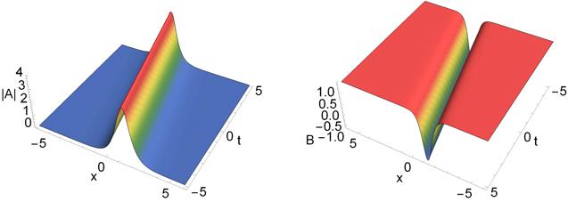
Figure 1. One-soliton solution. |
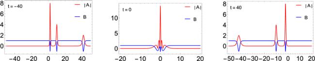
For N = 2, since the explicit expression of the two-soliton solution is quite complex, we omit the detailed calculation and give the figures with some parameters chosen as ${\alpha }_{1}={\beta }_{1}=1,{\alpha }_{2}={\beta }_{2}={\rm{i}},{\lambda }_{1}={\rm{i}},{\lambda }_{2}=\tfrac{1}{2}{\rm{i}}$. It can be seen from figure 2 that the solution is a two-bright-dark soliton solution with collisions at point (0, 0). In particular, we can see from figure 3 that collisions are elastic since waves do not undergo shape-changing collisions as they propagate.
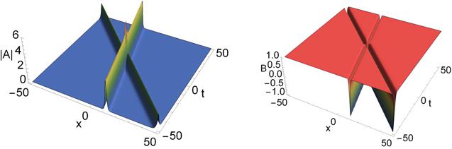
Figure 2. Two-soliton solution. |
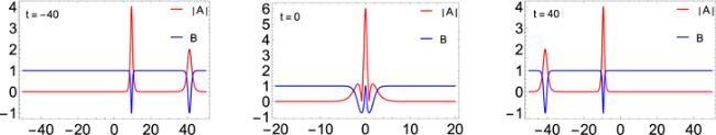
Figure 3. Two-soliton elastic collision. |
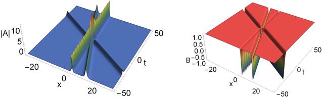
Figure 4. Three-soliton solution. |
Figure 5. Three-soliton elastic collision. |
5. Conclusion and discussion
It is of great significance to investigate the solutions of the AB system, which may help to better understand ultra-short optical pulse propagation in nonlinear optics. The AB system is the negative flow of the Lax pair, so it is very difficult to deal with the system using the Riemann–Hilbert approach. The potential B is at the diagonal position of the matrix V, which is different from other models such as focusing nonlinear Schrödinger equation. Therefore, we need to assume function B decays to 1 as x → ∞ and use evolution equations of the Jost function with respect to both x and t when reconstructing the potentials. For the direct scattering problem, the analyticities, symmetries and asymptotic behaviors of the Jost solutions, scattering matrix and discrete spectra, are established by resorting to the inverse scattering transformation. The inverse problems are formulated and solved with the aid of the matrix Riemann–Hilbert problems, and the reconstruction formulas are obtained. And from that we construct the muti-bright-dark soliton solutions to the AB system. The collisions are elastic, which means that the solitons are capable of propagating over long distances without shape-changing and thus are quite important in optical fiber communication. We also try to find out whether inelastic (shape-changing) collisions exist in the multi-soliton collisions of the AB system. In addition, the study of non-zero boundary problems by the Riemann–Hilbert method has aroused great interest. In the future, we will focus on finding some other explicit solutions such as the breathers, rogue wave solutions and others by using the inverse scattering method with nonzero boundary conditions.