


1. Introduction
Quantum algorithms are widely applied in quantum information processing, due to the exponential speedup effect compared to their classical counterparts [1–5]. As a useful tool for implementing quantum algorithms, graphs have been investigated to support many quantum algorithms, such as quantum search, PageRank algorithms, etc [6–11]. Although quantum algorithms are better than their classical counterparts in principle, the advantages of quantum algorithms are diminished when considering realistic physical conditions. To date, ion traps, atoms and superconducting qubits [12–14] have usually been used as a platform to realize quantum information tasks. These systems are quite sensitive to environmental dissipation. The quantum coherence of a system is weak if an external disturbance can destroy it [15, 16], which is a major obstacle to quantum computation. Therefore, it is important to study how to implement a quantum computation accompanied by environmental dissipation.
The interactions between quantum systems and environments can be classified into various noises, such as memoryless white noise where the environment is often Markovian, and color noise with memory in which the environment behaves in a non-Markovian way [15, 16]. Many studies illustrate the role played by the environment as a simple Markovian one and obtain similar results between experimental outcomes and theoretical analysis [15, 17, 18]. However, recent results reveal that non-Markovian scenarios also widely exist in reality. Typical examples include a single trapped ion interacting with an engineered reservoir [19, 20], spontaneous emission atomic dynamics in photonic crystals [21], microcavities coupling with a coupled-resonator optical waveguide or photonic crystals [22, 23], etc. The essential difference between Markovian and non-Markovian environments lies in whether the probability or energy can flow back from the environment to the quantum system. Studies have demonstrated that the dynamics of the quantum system are quite different between Markovian and non-Markovian scenarios [24–30]. Therefore, in the non-Markovian case, the environment cannot be viewed as a leakage only, but it is capable of intentionally controlling the interacting quantum system [19, 20, 22, 30]. Recently, dissipative quantum-state engineering and quantum computation have attracted much attention. A large variety of strongly correlated states can be realized through dissipation [31]. A mechanical oscillator cooled close to its ground state is revealed by controlling the coupling to the dissipation [32]. A dissipation-assisted proposal to transfer an arbitrary quantum-state directionally is provided [33]. By engineering the steady-state of a sensor, quantum sensing under dissipation is realized [34]. High-fidelity nonclassical states are generated by dissipative quantum-state engineering [35], and autonomous quantum-state transfer over a long distance is achieved [36]. The above discussion motivates us to consider whether we can carry out a quantum algorithm accurately even if the influences from the environment are not negligible.
In this paper, we implement a fast quantum search by engineering the surrounding environment of the quantum system. A platform for fast quantum search is constructed with two-level atoms. Through engineering the interaction between quantum systems and non-Markovian environments, quantum search algorithms can be run efficiently due to the memory backflow. For comparison, we also show that the quantum search cannot be executed in the Markovian environment due to the irreversible dissipation. Finally, we discuss the possible experimental realizations of the fast quantum search. A quantum search based on ultracold atoms is introduced in detail.
2. Review of fast quantum search
The searching problem aims to find the target data point in one unsorted database. If the number of data points in the database is N, the success probability of finding the target data point is 1/N with a random guess. The average time of queries to find the target data point is N/2, when considering the time of the random guess is just ‘1’ in the best case and N in the worst case. When a quantum correlation was introduced into the algorithms, Grover developed a quantum search algorithm from the quantum circuit model [4]. It has been verified analytically that the target data point can be found with considerable probability through the use of order $\sqrt{N}$ queries. Some groups have experimentally demonstrated such results in different platforms, e.g. nuclear magnetic resonance [37, 38], optical implementation [39], ion trap [40], nitrogen-vacancy centers [41] and superconducting systems [42]. The involved numbers of data points in these experimental demonstrations are not large enough, whereas small decoherence in each component may accumulate into large decoherence and affect search results when the quantum systems become larger. The disappearance of quantum coherence may lead to wrong answers in the search outcome.
Recently, researchers verified that quantum speedup can also be reflected in the continuous-time quantum walk (CTQW) search algorithms on the graphs [6–9]. Compared to those in Grover’s search algorithms, there is no need for logic gate operations in the CTQW search algorithms. The theoretical results [8] have shown that for one d-dimensional cubic lattice, the target vertex in the graph can be found at the time of order $O(\sqrt{N})$ with d > 4, at the time of order $O(\sqrt{N}\mathrm{log}N)$ with d = 4, and no speedup with d < 4. In addition, researchers found that for graphs with low connectivity [6, 7, 9], the target vertex was also found through the delicate design of the transition rate among the adjacent vertices in the graphs. A typical example is the joined complete graph [7]. Recent investigations have verified that a fast quantum search can be realized in such a graph having low connectivity, which was previously thought impossible. A diagram of this joined complete graph is shown in figure 1.
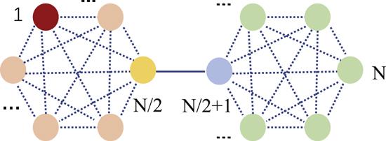
Figure 1. Diagram of the joined complete graph. Target vertex is in red and labeled as ‘1’. Other vertices in different colors represent different groups. For this joined complete graph, we can use a 5D subspace to obtain an optimal fast quantum search. Symbol ‘⋯’ denotes too many vertices, which are not shown. |
As shown in figure 1, the target vertex is drawn in red and labeled as ‘1’. The left and right parts of these graphs are two complete graphs that contain N/2 vertices. To illustrate the N vertices in the graph, we use dotted lines to represent enormous connections between every two vertices in the complete graphs. The left and right complete graphs are connected by only one edge, so we use a solid line to indicate this. For this graph, we can use computation basis states ∣ai⟩i=1,⋯,N. The state ∣ai⟩ is ${\left(0,\cdots ,1,\cdots ,0\right)}^{{\rm{T}}}$ where the ith element is nonzero. In the description of the graph, this state corresponds to the ith vertex. We choose the first vertex as the target vertex for convenience. Thus, the target vertex is $| w\rangle =| {a}_{1}\rangle ={\left(\mathrm{1,0},\cdots ,0\right)}^{{\rm{T}}}$. Considering the transition rate as γ, the Hamiltonian used for the fast quantum search is Hg = − γA − ∣w⟩⟨w∣ where the adjacent matrix A describes the connections between the vertices. The term − ∣w⟩⟨w∣ is often regarded as the ‘oracle’ Hamiltonian. The Hamiltonian Hg is expressed in matrix form as,
$\begin{eqnarray*}{H}_{g}=-\gamma \left(\begin{array}{cccccccc}1/\gamma & 1 & \cdots & 1 & 0 & \cdots & \quad & 0\\ 1 & 0 & \quad & \vdots & \vdots & \quad & \quad & \vdots \\ \vdots & \quad & \ddots & 1 & 0 & \quad & \quad & \vdots \\ 1 & \cdots & 1 & 0 & 1 & 0 & \cdots & 0\\ 0 & \cdots & 0 & 1 & 0 & 1 & \cdots & 1\\ \vdots & \quad & \quad & 0 & 1 & 0 & \quad & \vdots \\ \quad & \quad & \quad & \vdots & \vdots & \quad & \ddots & 1\\ 0 & \cdots & \quad & 0 & 1 & \cdots & 1 & 0\end{array}\right).\end{eqnarray*}$
In this N × N matrix, the top left N/2 × N/2 matrix describes the interactions in the left complete graph, and the right bottom N/2 × N/2 matrix shows the interactions in the right complete graph. In addition to these top left and right bottom N/2 × N/2 matrices, only two elements in the remaining matrix Hg are nonzero (the N/2-th row, the (N/2 + 1)-th column, and the (N/2 + 1)-th row, the N/2-th column in the matrix). These two elements represent the connection between the N/2-th vertex and (N/2+1)-th vertex in the joined complete graph.
When discussing the fast quantum search in the graph, the initial state is commonly chosen as one equal superposition of all basis states $| s\rangle =1/\sqrt{N}{\sum }_{i=1}^{N}| {a}_{i}\rangle $, which means that there is no knowledge about the target vertex. When the search process begins, we focus on the magnitude $| \langle w| {{\rm{e}}}^{-{\rm{i}}{H}_{g}t}| s\rangle {| }^{2}$, which represents the success probability to find the target vertex. For this joined complete graph, as revealed in [7], the original basis states are grouped identically. One can obtain the basis of a 5D subspace as $\{| 1\rangle ,1/\sqrt{N/2-2}(| 2\rangle +| 3\rangle \cdots +| N/2-1\rangle ),| N/2\rangle ,| N/2\,+1\rangle ,1/\sqrt{N/2-1}(| N/2+2\rangle \cdots +| N\rangle )\}\,.$ The corresponding matrix in this subspace is,
$\begin{eqnarray}{H}_{g}^{\prime} =-\gamma \left(\begin{array}{ccccc}1/\gamma & \sqrt{\tfrac{N}{2}-2} & 1 & 0 & 0\\ \sqrt{\tfrac{N}{2}-2} & \tfrac{N}{2}-3 & \sqrt{\tfrac{N}{2}-2} & 0 & 0\\ 1 & \sqrt{\tfrac{N}{2}-2} & 0 & 1 & 0\\ 0 & 0 & 1 & 0 & \sqrt{\tfrac{N}{2}-1}\\ 0 & 0 & 0 & \sqrt{\tfrac{N}{2}-1} & \tfrac{N}{2}-2\end{array}\right).\end{eqnarray}$
When the perturbation method is employed, one can find the appropriate transition rate γ = 2/N to reach the optimal fast quantum search [7]. The largest success probability to find the target vertex is 50%.
Even though the theoretical results have provided good performance in the quantum search on the graphs, only the related experimental demonstrations [43] with the simplest case have been reported recently. This is because the connections between vertices in the graphs are complicated, and easily affected by the surrounding environment. Under realistic conditions, the unavoidable dissipation diminishes the coherence and makes the system work at a steady condition within a short time [43, 44]. Quantum walk search algorithms under decoherence have been studied theoretically in detail [45]. It is concluded that the existence of decoherence leads to more time and lower successful search probability in the search process.
Based on the discussion above, it is clearly shown that quantum search algorithms can have good performance in theory, but actual realizations may have strong limitations due to decoherence. Therefore, exploring how to execute fast quantum search algorithms under decoherence becomes an interesting task. An effective way is to use the existing quantum algorithms with consideration of decoherence and make every effort to reduce the influence of this decoherence. Recent work regarding the realization of quantum logic in a noisy environment motivates us to engineer dissipation for quantum search algorithms [30]. It is necessary that we know the noise spectrum of the environment, and engineer the corresponding environment by using open quantum system theory. In our study, we focus on this method and ensure the effective operation of existing quantum algorithms.
3. Quantum search in atomic systems
In this section, we construct the joined complete graphs based on atomic ensembles to realize a fast quantum search. We consider an atomic system as illustrated in figure 2(a). The two internal states of each atom are depicted as spin up ∣ ↑ ⟩ and spin down ∣ ↓ ⟩. The whole system comprises two symmetric subsystems and each subsystem has N/2 atoms. We assume that any two atoms in the subsystem have identical interactions γ. Each subsystem corresponds to a complete graph and the subsystems are connected through an atomic interaction γ, e.g. the interaction between the N/2-th and the (N/2 + 1)-th atoms in figure 2(a), and we assume that there are no interactions between the other atoms of the two subsystems. The atomic excitation (∣ ↑ ⟩) can be transferred among atoms through atomic interaction. Each time the excitation is transferred to atom 1 (the red one in figure 2), the system can accumulate a π phase shift, which is just the functionality of Oracle in quantum search. The phase shift can be implemented by applying a magnetic field, which will be introduced in section 5 in detail. The Hamiltonian of the system can be written as,1 )). The Hamiltonian H0 for arbitrary N can also be obtained in the same way, and it is also similar to the search Hamiltonian of the joined complete graph with N vertices (equation (1 )). The fast quantum search can thus be implemented in the two-level atomic system with Hamiltonian H0. One can obtain the search Hamiltonian H0 (equation (2 )) by utilizing ultracold atoms, which will be discussed below.
$\begin{eqnarray}\begin{array}{rcl}{H}_{0} & = & -\gamma [\displaystyle \sum _{i=1,i\lt j}^{i,j=\tfrac{N}{2}}(| \uparrow {\rangle }_{i}\langle \downarrow | | \downarrow {\rangle }_{j}\langle \uparrow | +{\rm{H}}.{\rm{c}}.)\\ & & +\,(| \uparrow {\rangle }_{\tfrac{N}{2}}\langle \downarrow | | \downarrow {\rangle }_{\tfrac{N}{2}+1}\langle \uparrow | +{\rm{H}}.{\rm{c}}.)\\ & & +\,\displaystyle \sum _{i=\tfrac{N}{2}+1,i\lt j}^{i,j=N}(| \uparrow {\rangle }_{i}\langle \downarrow | | \downarrow {\rangle }_{j}\langle \uparrow | +\ {\rm{H}}.{\rm{c}}.)]-| \uparrow {\rangle }_{1}\langle \uparrow | .\end{array}\end{eqnarray}$
We assume that atoms are initially in an equal superposition state $| {{\rm{\Psi }}}_{0}(0)\rangle =1/\sqrt{N}{\sum }_{j=1}^{N}| j\rangle $. Here, state ∣j⟩ =∣ ↓ 1 ↓ 2 ⋯ ↑ j ⋯ ↓ N⟩ describes that atom j (j = 1, 2, ⋯ ,N) is in the spin-up state ∣ ↑ ⟩ and the others are in spin-down states ∣ ↓ ⟩. Specifically, as mentioned above, ∣1⟩ is the state we are searching for. As the interactions between quantum systems and environments are not included in Hamiltonian H0, the system governed by H0 is a closed system with only one excitation in the evolution. The computational basis states can be expressed as {∣1⟩, ∣2⟩, ⋯ ,∣N − 1⟩, ∣N⟩}. The Hamiltonian H0 for N = 8 atoms (figure 2(b)) can be expressed in 5D subspace as, $\begin{eqnarray*}{H}_{0}=-\gamma \left(\begin{array}{ccccc}1/\gamma & \sqrt{2} & 1 & 0 & 0\\ \sqrt{2} & 1 & \sqrt{2} & 0 & 0\\ 1 & \sqrt{2} & 0 & 1 & 0\\ 0 & 0 & 1 & 0 & \sqrt{3}\\ 0 & 0 & 0 & \sqrt{3} & 2\end{array}\right),\end{eqnarray*}$
which is similar to the search Hamiltonian of the joined complete graph with eight vertices (equation (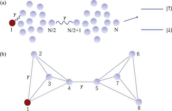
Figure 2. (a) Illustration of the atomic system composed of two symmetric subsystems. Each subsystem comprises N/2 atoms, and each atom has two internal states, ∣ ↑ ⟩ and ∣ ↓ ⟩. Atoms in the subsystem interact with each other through identical interactions γ. Two subsystems are coupled through the interaction between the N/2-th and the (N/2 + 1)-th atoms. (b) Specific example with eight atoms for the model depicted in (a). |
The general state of the atomic system can be expressed as $| {{\rm{\Psi }}}_{0}(t)\rangle ={\sum }_{j=1}^{N}{C}_{j}(t)| j\rangle $, and evolves through Schrödinger’s equation $| {\dot{{\rm{\Psi }}}}_{0}(t)\rangle =-{\rm{i}}{H}_{0}| {{\rm{\Psi }}}_{0}(t)\rangle $. When N = 8 and γ = 0.25 (this value of γ is the optimal one in [7]), we get P1 = ∣C1(t)∣2, as shown in figure 3(a) (blue solid line), which is the probability of atoms in state ∣1⟩. From figure 3(a), it is found that there is almost a 50% success probability for searching the marked state ∣1⟩ at time t = 3.2 ≈ π. Similarly, the success probability reaches 50% at time $t=4.4\approx \sqrt{2}\pi $ for N = 16 and γ = 0.125 (which is also optimal, as shown in [7]), and illustrated in figure 3(a) (yellow line). The corresponding probability distributions Pj = ∣Cj(t)∣2 (j = 1, ⋯ ,N) for N = 8, t = 3.2 and N = 16, t = 4.4, are shown in figures 3(b) and (c) respectively. The above search results are similar to those in the study of joined complete graphs [7]. Similarly, with the demonstrations in joined complete graphs [7], for arbitrary atomic numbers N, the marked state ∣1⟩ can be successfully searched with 50% probability in a runtime of $O(\sqrt{N})$ under the Hamiltonian H0. A fast quantum search can be achieved by utilizing interaction H0 in atomic systems.
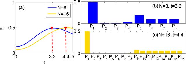
Figure 3. Success probability P1 = ∣C1(t)∣2 and probability distribution for quantum search in the atomic system. (a) Probabilities P1 for N = 8 (blue solid line) and N = 16 (yellow solid line) atoms are illustrated, respectively. (b) Probability distribution Pj(j = 1, ⋯ ,N) for N = 8 and t = 3.2. (c) Probability distribution Pj(j = 1, ⋯ ,N) for N = 16 and t = 4.4. |
The above demonstrations are discussed in the ideal case, in which we assume the atomic systems for realizing quantum algorithms are not affected by external environments. The influences induced by the environment are completely ignored, and the implementation of the quantum algorithm only depends on the evolution of the atomic system itself. However, a practical system inevitably interacts with environments, e.g. atomic spontaneous emissions, etc, where the evolution of the atomic system is consequentially influenced by the interacting environment. In many experiments, the theory of open quantum systems that considers the couplings between systems and environments is utilized to theoretically analyze the experimental results more accurately [15–23]. Therefore, realizations of quantum algorithms in practical systems need to be discussed based on the theory of open quantum systems. The interactions between atoms and environments should be included in the model of fast quantum search.
4. Quantum search with dissipation
In the following, we will study quantum search in dissipative environments. The interactions between atomic systems and environments will be considered. We assume that the environment is quantized into a collection of harmonic oscillators with frequencies ω. The interactions between atoms and environments can be described as,A ). The time correlation function $u(t-t^{\prime} )={\int }_{0}^{\infty }| g(\omega ){| }^{2}{{\rm{e}}}^{{\rm{i}}({\omega }_{\uparrow \downarrow }-\omega )(t-t^{\prime} )}{\rm{d}}\omega $, which takes into account the structure and memory effect of the environment, is introduced into the atomic evolution (see appendix A ). Different structured environments have their corresponding time correlation functions, which lead to various dynamic evolutions. Quantum search in atomic systems is influenced by environmental structure. In the following, first we study quantum search in Markovian environments. Then, we engineer memory backflow and discuss quantum search in non-Markovian environments.
$\begin{eqnarray}\begin{array}{l}{H}_{{\rm{I}}}=\displaystyle \sum _{j=1}^{N}({\displaystyle \int }_{0}^{\infty }g(\omega )| \uparrow {\rangle }_{j}\langle \downarrow | b(\omega ) \,\times \,{{\rm{e}}}^{{\rm{i}}({\omega }_{\uparrow \downarrow }-\omega )t}{\rm{d}}\omega +{\rm{H}}.{\rm{c}}.),\end{array}\end{eqnarray}$
where ω↑↓ is the transition frequency between atomic states ∣ ↑ ⟩ and ∣ ↓ ⟩. b(ω) denotes the annihilation operator of the environment. g(ω) is the coupling strength between the atom and the environment. The whole system including atoms and environments is evolved by Hamiltonian H = H0 + HI, and the total state can be generally expressed as, $\begin{eqnarray}\begin{array}{l}| {\rm{\Psi }}(t)\rangle =| {{\rm{\Psi }}}_{0}(t)\rangle | 0{\rangle }_{E}+| 0\rangle \,\times \,{\displaystyle \int }_{0}^{\infty }{C}_{\omega }(t){b}^{\dagger }(\omega )| 0{\rangle }_{E}{\rm{d}}\omega .\end{array}\end{eqnarray}$
Here, $| 0\rangle =| {\downarrow }_{1}\cdots {\downarrow }_{\tfrac{N}{2}}\cdots {\downarrow }_{N}\rangle $ is the atomic state without excitations. ∣0⟩E is the vacuum state of the environment. We initialize the excitation equally distributed among atoms and there is no excitation in the environment. The corresponding initial conditions can be expressed as ${C}_{j}(0)=1/\sqrt{N}(j=1,\cdots ,N),{C}_{\omega }(0)=0$. By substituting ∣$\Psi$(t)⟩ and H into Schrödinger’s equation, we can obtain equations of motion (see appendix Markovian scenarios
In the Markovian approximation, the coupling spectrum ∣g(ω)∣2 of the environment is almost flat and independent of modes. This noise spectrum has been widely applied in the study of open quantum systems [15–18]. We consider the spectrum of the environment as ∣g(ω)∣2 = Γ/π. After substituting ∣g(ω)∣2 into equation (A4 ) (appendix A ), we obtain the corresponding time correlation function $u(t-t^{\prime} )\,=2{\rm{\Gamma }}\delta (t-t^{\prime} )$. In the derivation of $u(t-t^{\prime} )$, we have shifted the integral limit (0, + ∞ ) of equation (A4 ) (appendix A ) to (−ω↑↓, + ∞ ), and extended the lower limit to − ∞ as a good approximation due to the large optical frequency ω↑↓. Therefore, the integral terms $-{\sum }_{j=1}^{N}{\int }_{0}^{t}u(t-t^{\prime} ){C}_{j}(t^{\prime} ){\rm{d}}t^{\prime} $ of equations (A3a )–(A3e ) (appendix A ), which describe the interaction between atoms and environments, can be replaced by $-{\rm{\Gamma }}{\sum }_{j=1}^{N}{C}_{j}(t)$. We can simulate the quantum search on atoms that are coupled with Markovian environments. The simulation results are shown in figure 4 (red dashed lines). In the Markovian approximation, the environment is memoryless and the energy is irreversibly dissipated into the surroundings. It is found that the success probability P1 = ∣C1(t)∣2 representing the probability for atoms in the marked state ∣1⟩, decays exponentially due to the loss. Therefore, the quantum search cannot be executed with atoms coupled with Markovian environments.
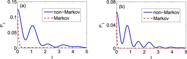
Figure 4. Success probability P1 = ∣C1(t)∣2 for quantum search in the atomic system. Probabilities P1 correspond to Markovian (red dashed lines) and non-Markovian environments (blue solid lines) are presented, respectively. We assume the spectra of the non-Markovian environments are Lorentzian spectra. (a) Success probability for N = 8, γ = 0.25, Γ = 1 and λ = Γ. (b) Success probability for N = 16, γ = 0.125, Γ = 1 and λ = Γ. |
Non-Markovian scenarios with Lorentzian spectra
We have studied quantum search in Markovian environments. Although the experiments can be well described with Markovian theory in many cases, color noise is required to describe the environment more precisely due to the complexity of the realistic environment [15, 16, 19–23]. In many situations, the structure of environments cannot be ignored and one needs to consider the specific spectra ∣g(ω)∣2. One of the common spectra for color noise is a Lorentzian spectrum, which is widely applied in atom-cavity systems [46–49], photonic crystals [21, 48], etc. Lorentzian noise can also be shaped by filtering white noise with a cavity [50]. Different from the Markovian scenarios, non-Markovian environments have memory effects and the energy leaked into the environments can flow back to the system. Furthermore, some good performances in quantum information processing under this Lorentzian noise have been reported. In the following, we study quantum search in non-Markovian environments and demonstrate that an ideal quantum search can be achieved by designing environments. A Lorentzian spectrum can be written as,5 ) into (A4 ) (appendix A ) and obtain the corresponding time correlation function:6 ) into the equations of motion (equations (A3a )–(A3e ) in appendix A ), we simulate quantum search on atoms in Lorentzian environments. As illustrated in figure 4, for Lorentzian spectra with finite widths λ, the success probabilities P1 (blue solid lines) oscillate and decay slowly with time, which is completely different from the Markovian cases (red dashed lines). As previously stated, a narrower spectral width implies a stronger memory effect. As λ decreases, more energy that is dissipated into the environments can flow back to the system. Figures 5(a) and (c) exhibit the corresponding success probabilities P1 under different spectral widths λ, when the atomic numbers are N = 8 and N = 16. From figure 5, one finds that the success probability P1 increases as λ decreases. When the spectral width λ decreases to 0.001Γ, the success probability on a time scale $O(\sqrt{N})$ can almost be revived to 50%. Figures 5(b) and (d) describe the corresponding probability distributions for different λ, when N = 8, t = 3.2 and N = 16, t = 4.4. The probability PE is the energy dissipated into the environment and PE = 1 − ∑jPj. As previously stated, in figures 5(b) and (d), less net energy loss PE occurs as λ decreases. Furthermore, it is also found that the probability distribution may be influenced by the interaction between atoms and the environment. On the one hand, the probability distributions (λ = 0.1Γ and λ = 0.01Γ) that include couplings to the environment, are quite different from those in the ideal case (figures 3(b) and (c)), and on the other hand, different spectral widths λ result in various probability distributions. Specifically, when λ decreases to 0.001Γ, the probability distributions Pj(j = 1, ⋯ ,N) are almost the same as the distributions in figures 3(b) and (c).
$\begin{eqnarray}| g(\omega ){| }^{2}=\displaystyle \frac{{\rm{\Gamma }}}{\pi }\displaystyle \frac{{\lambda }^{2}}{{\left(\omega -{\omega }_{\uparrow \downarrow }\right)}^{2}+{\lambda }^{2}},\end{eqnarray}$
where Γ and λ represent the strength and spectral width of the coupling between the atomic transition and environments. In particular, the spectral width λ is inversely proportional to the memory time of environments. When λ tends to infinity, the environment becomes memoryless and the spectrum ∣g(ω)∣2 is equal to a constant value Γ/π. One can substitute equations ( $\begin{eqnarray}u(t-t^{\prime} )={\rm{\Gamma }}\lambda {{\rm{e}}}^{-\lambda | t-t^{\prime} | }.\end{eqnarray}$
By substituting equation (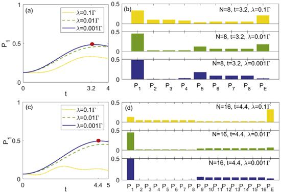
Figure 5. Success probability P1 = ∣C1(t)∣2 and probability distribution for quantum search in the atomic system. In Lorentzian environments, the probabilities P1 and probability distributions Pj(j = 1, ⋯ ,N) and PE corresponding to different spectral widths λ = 0.1Γ, λ = 0.01Γ and λ = 0.001Γ are presented, respectively. (a) Success probability for N = 8 and γ = 0.25. (b) Probability distribution for N = 8, t = 3.2 and γ = 0.25. (c) Success probability for N = 16 and γ = 0.125. (d) Probability distribution for N = 16, t = 4.4 and γ = 0.125. |
It should be noted that the interaction between atoms and external environments has been considered in this section. From the above calculations, we find that, when couplings between atoms and environments are included, quantum noise usually causes negative effects for the implementation of the quantum search algorithm (as depicted in figures 4 and 5). Therefore, it is hard to realize fast quantum search in practical systems. However, our studies show that one can achieve a fast quantum search by manipulating the spectral width λ of the environment. A success probability of 50% is acquired on a time scale $O(\sqrt{N})$. By comparison, the results in sections 2 and 3 only exist in ideal models, where the couplings between atoms and environments are excluded and the effect of quantum noise is ignored. Therefore, one needs to use an environmental engineering approach to realize fast quantum search in practical systems considering quantum noise.
5. Experimental realizations
In the following, we discuss the experimental realizations of fast quantum search. First, we show how to realize the ideal quantum search Hamiltonian H0 without consideration of the surrounding environment. As shown in figure 4, the ideal fast quantum search disappears when white noise is considered. This noise is commonly studied in quantum information experiments [15, 17, 18]. Then, we provide a way to engineer the environment, which changes the white noise to the Lorentzian environment. The search Hamiltonian equation (2 ) can be obtained through Heisenberg XY interactions. The Heisenberg XY model, which has been intensively investigated in both theory and experiment, can be realized in cold atoms [51, 52], quantum dot spins [53], cavity quantum electrodynamics [54], etc.
We consider the model in figure 2(b) as an illustration. Eight ultracold bosonic atoms are trapped inside an optical lattice. The four atoms on the right (left) side constitute vertices of a regular tetrahedron in 3D space. For sufficiently strong potential and low temperatures, the low-energy Hamiltonian is [51, 52],7 )) can be written as [52],8 ), the overall energy shifts caused by lattice potential are taken into account. Designs of the inhomogeneous magnetic profiles have been investigated in many theoretical and experimental studies [55–60]. Magnetic structures with different geometries have been experimentally realized [55–57, 59, 60]. For example, a magnetic field distributed by cosine functions in 1D space can be acquired by exploiting the fringe field produced by ferromagnetic strips [56]. Applying a uniform magnetic field to the nonplanar 2D electron gas can generate a step-structured magnetic field [57], a periodic solenoidal focusing magnetic field can be defined by periodic step functions [58], a film of superconducting material with the desired pattern [59], and anti-Helmholtz coil pairs [60] can also be utilized to obtain structured magnetic fields. Therefore, we can generate the magnetic field with a step function distribution in the space. The magnetic field at atomic site j = 1 may be zero and different from fields at other atomic sites. By applying an external magnetic field to atoms, except for atom j = 1, one can compensate for the energy shifts of the atoms j ≠ 1. The expressions of parameters J, $J^{\prime} $, D and B are,2 )) for N = 8. Here, the Hilbert space for N atoms is 2N. In our realization with N atoms, we only make use of the first excitation subspace with N dimensions. The ‘oracle’ Hamiltonian is required when searching the target vertex on the graph. It is convenient to realize this Hamiltonian by the design of the distribution of magnetic field as stated above. Moreover, our design can realize a programable quantum search by changing the distribution of the magnetic field. We can achieve the quantum search of any vertex on the graph.
$\begin{eqnarray}\begin{array}{rcl}H^{\prime} & = & {H}_{0}^{{\prime} }+V,\\ {H}_{0}^{{\prime} } & = & \displaystyle \frac{1}{2}\displaystyle \sum _{j,\sigma }{U}_{\sigma }{n}_{j\sigma }({n}_{j\sigma }-1)+{U}_{\uparrow \downarrow }\displaystyle \sum _{j}{n}_{j\uparrow }{n}_{j\downarrow },\\ V & = & -\displaystyle \sum _{\langle {ij}\rangle \sigma }({t}_{\sigma }{a}_{i\sigma }^{\dagger }{a}_{j\sigma }+{\rm{H}}.{\rm{c}}.),\end{array}\end{eqnarray}$
where ⟨ij⟩ denotes the nearest neighbor atoms. ${a}_{j\sigma }^{\dagger }$ and ajσ are the bosonic creation and annihilation operators for atom j with spin σ (σ = ↑ or ↓ ), respectively, and we have ${n}_{j\sigma }={a}_{j\sigma }^{\dagger }{a}_{j\sigma }$. The on-site interaction energies are given by Uσ and U↑↓. tσ represents the spin-dependent tunneling energy between neighboring atoms in the lattice. In the Mott insulator phase, where ∣tσ∣ ≪ Uσ, U↑↓ and nj↑ + nj↓ = 1, the Hamiltonian (equation ( $\begin{eqnarray}\begin{array}{rcl}H^{\prime} & = & -\sum _{\langle {ij}\rangle }(J{\vec{\sigma }}_{i}{\vec{\sigma }}_{j}+J^{\prime} {\sigma }_{{iz}}{\sigma }_{{jz}})\\ & & +\sum _{j}\left[\displaystyle \frac{D}{2}{\left({\sigma }_{{jz}}\right)}^{2}-B{\sigma }_{{jz}}\right],\end{array}\end{eqnarray}$
where ${\sigma }_{{jx}}={a}_{j\uparrow }^{\dagger }{a}_{j\downarrow }+{a}_{j\downarrow }^{\dagger }{a}_{j\uparrow }$, ${\sigma }_{{jy}}=-{\rm{i}}({a}_{j\uparrow }^{\dagger }{a}_{j\downarrow }-{a}_{j\downarrow }^{\dagger }{a}_{j\uparrow })$ and σjz = nj↑ − nj↓. In equation ( $\begin{eqnarray*}\begin{array}{rcl}J & = & 2{t}_{\uparrow }{t}_{\downarrow }/{U}_{\uparrow \downarrow },\\ J^{\prime} & = & -{\left({t}_{\uparrow }+{t}_{\downarrow }\right)}^{2}/{U}_{\uparrow \downarrow }+2{{t}_{\uparrow }}^{2}/{U}_{\uparrow }+2{{t}_{\downarrow }}^{2}/{U}_{\downarrow },\\ D & = & {U}_{\uparrow }+{U}_{\downarrow }-2{U}_{\uparrow \downarrow },\\ B & = & ({\mu }_{\uparrow }+6{{t}_{\uparrow }}^{2}/{U}_{\uparrow })-({\mu }_{\downarrow }+6{{t}_{\downarrow }}^{2}/{U}_{\downarrow }).\end{array}\end{eqnarray*}$
Here, μσ is the potential for spin σ. Since the optical lattice is formed by the standing-wave laser beams, the parameters J, $J^{\prime} $, D and B can easily be controlled by manipulating the strengths of trapping laser beams and changing the atomic scattering lengths [51]. By appropriately engineering the parameters (e.g. Uσ = 2U↑↓, D/2 = − B), one can finally achieve the following Hamiltonian: $\begin{eqnarray*}\begin{array}{l}H^{\prime} =-\gamma \displaystyle \sum _{\langle {ij}\rangle }({a}_{i\uparrow }^{\dagger }{a}_{i\downarrow }{a}_{j\downarrow }^{\dagger }{a}_{j\uparrow }+{a}_{i\downarrow }^{\dagger }{a}_{i\uparrow }{a}_{j\uparrow }^{\dagger }{a}_{j\downarrow })-{a}_{1\uparrow }^{\dagger }{a}_{1\uparrow },\end{array}\end{eqnarray*}$
which is equivalent to the Hamiltonian H0 (equation (Since the atoms inevitably interact with external environments, the realistic systems are open quantum systems. In the previous discussion, we demonstrated that when a system is coupled with Lorentzian environments, one can realize fast quantum search by engineering environments. As reported in some experiments, the environments are treated as Markovian cases with white noise. The dynamics of the atomic system interacting with a Lorentzian environment can be equivalently described by the coherent coupling between the system and pseudomodes, with the latter leaking into an independent Markovian environment [46–48]. Calculation details related to the dynamics of atoms within the pseudomode method are provided in appendix B . The frequency and decay rate of the pseudomode, which are determined by noise spectrum equation (5 ), are ω↑↓ and 2λ, respectively (appendix B ). The coupling strength between atoms and the pseudomode is ${\rm{\Omega }}=\sqrt{{\rm{\Gamma }}\lambda }$ (appendix B ). It can easily be found that the equivalent coupling strength Ω gets weaker as the spectral width λ becomes smaller. Fewer atomic excitations are transferred to the pseudomode and dissipated, due to the net effect of energy backflow. Through narrowing the spectral width λ, the atomic system can be finally viewed as decoupled from the pseudomode, and one can thus realize an ideal quantum search. The Lorentzian environments can be experimentally constructed by leaving a lossy cavity in the Markovian environment, which can filter the input white noise into color noise with the Lorentzian spectrum [46–48, 50]. By manipulating the cavity parameters (e.g.,cavity transmissivity and reflectivity, quality factor, etc), one can engineer the Lorentzian environment.
6. Conclusion
We studied the realization of fast quantum search in atomic systems. Through constructing a joined complete graph in atoms, a fast quantum search of runtime $O(\sqrt{N})$ is realized with a success probability of 50%. Furthermore, we take into account the influence of dissipation, which arises due to the inevitable coupling of a system with its environment. When the system interacts with a Markovian environment, energy can be irreversibly leaked into external environments. The quantum speedup effect is washed out by dissipation, thus a fast quantum search cannot be achieved. However, a completely different phenomenon can arise in our engineered non-Markovian environments. Through engineering Lorentzian environments, one can re-implement an ideal fast quantum search due to the energy backflow from the environment to the system. Finally, we also discuss the possible experimental realizations based on ultracold atoms. As dissipation is one of the strongest adversaries in quantum computation, our work provides a possible path for realizing fast quantum search in practical systems. Our proposal here is based on engineering of the environment. Other ways to diminish decoherence may work well through engineering the system Hamiltonian. One representative method is dynamical decoupling, which has been widely applied in the preservation of coherence in quantum systems [61–66]. When applying dynamic decoupling to our system, we need to engineer the incident Hamiltonian to overcome a certain kind of noise. We will study this in the near future.
Acknowledgments
This work was supported by the National Key R&D Program of China (Grant No. 2017YFA0303800) and the National Natural Science Foundation of China (Grant Nos. 11 604 014 and 11 974 046).
Appendix A. Time evolutions of atoms in dissipative environments
The total system comprises N two-level atoms and a quantized environment. Through deriving Schrödinger's equation $| \dot{{\rm{\Psi }}}(t)\rangle =-{\rm{i}}H| {\rm{\Psi }}(t)\rangle $, we obtain equations of motion as follows:A1f ) and substituting the initial condition Cω(0) = 0, we obtain:A2 ) into equations (A1a )-(A1e ), we obtain:
$\begin{eqnarray}\begin{array}{l}{\dot{C}}_{1}(t)=-{\rm{i}}\gamma \displaystyle \sum _{i=2}^{i=\tfrac{N}{2}}{C}_{i}(t)\\ -{\rm{i}}{\displaystyle \int }_{0}^{\infty }{C}_{\omega }(t)g(\omega ){{\rm{e}}}^{{\rm{i}}({\omega }_{\uparrow \downarrow }-\omega )t}{\rm{d}}\omega +{\rm{i}}{C}_{1}(t),\\ \mathrm{when}\quad j=2,\cdots ,N/2-1,\end{array}\end{eqnarray}$
$\begin{eqnarray}\begin{array}{l}{\dot{C}}_{j}(t)=-{\rm{i}}\gamma \displaystyle \sum _{i=1,i\ne j}^{i=\tfrac{N}{2}}{C}_{i}(t)\\ -{\rm{i}}{\displaystyle \int }_{0}^{\infty }{C}_{\omega }(t)g(\omega ){{\rm{e}}}^{{\rm{i}}({\omega }_{\uparrow \downarrow }-\omega )t}{\rm{d}}\omega ,\end{array}\end{eqnarray}$
$\begin{eqnarray}\begin{array}{l}{\dot{C}}_{\displaystyle \frac{N}{2}}(t)=-{\rm{i}}\gamma \displaystyle \sum _{i=1,i\ne \tfrac{N}{2}}^{i=\tfrac{N}{2}+1}{C}_{i}(t)\\ -{\rm{i}}{\displaystyle \int }_{0}^{\infty }{C}_{\omega }(t)g(\omega ){{\rm{e}}}^{{\rm{i}}({\omega }_{\uparrow \downarrow }-\omega )t}{\rm{d}}\omega ,\end{array}\end{eqnarray}$
$\begin{eqnarray}\begin{array}{l}{\dot{C}}_{\tfrac{N}{2}+1}(t)=-{\rm{i}}\gamma \displaystyle \sum _{i=\tfrac{N}{2},i\ne \tfrac{N}{2}+1}^{i=N}{C}_{i}(t)\\ -{\rm{i}}{\displaystyle \int }_{0}^{\infty }{C}_{\omega }(t)g(\omega )\\ \quad \times {{\rm{e}}}^{{\rm{i}}({\omega }_{\uparrow \downarrow }-\omega )t}{\rm{d}}\omega ,\\ \mathrm{when}\quad j=N/2+2,\cdots ,N,\end{array}\end{eqnarray}$
$\begin{eqnarray}\begin{array}{l}{\dot{C}}_{j}(t)=-{\rm{i}}\gamma \displaystyle \sum _{i=\tfrac{N}{2}+1,i\ne j}^{i=N}{C}_{i}(t)\\ -{\rm{i}}{\displaystyle \int }_{0}^{\infty }{C}_{\omega }(t)g(\omega ){{\rm{e}}}^{{\rm{i}}({\omega }_{\uparrow \downarrow }-\omega )t}{\rm{d}}\omega ,\end{array}\end{eqnarray}$
$\begin{eqnarray}{\dot{C}}_{\omega }(t)=-{\rm{i}}\sum _{i=1}^{N}{C}_{i}(t){g}^{* }(\omega ){{\rm{e}}}^{-{\rm{i}}({\omega }_{\uparrow \downarrow }-\omega )t}.\end{eqnarray}$
By integrating the equation ( $\begin{eqnarray}{C}_{\omega }(t)=-{\rm{i}}\sum _{i=1}^{N}{\int }_{0}^{t}{C}_{i}(t^{\prime} ){g}^{* }(\omega ){{\rm{e}}}^{-{\rm{i}}({\omega }_{\uparrow \downarrow }-\omega )t^{\prime} }{\rm{d}}t^{\prime} .\end{eqnarray}$
After substituting equation ( $\begin{eqnarray}\begin{array}{l}{\dot{C}}_{1}(t)=-{\rm{i}}\gamma \displaystyle \sum _{i=2}^{i=\tfrac{N}{2}}{C}_{i}(t)\\ -\,\displaystyle \sum _{i=1}^{N}{\displaystyle \int }_{0}^{t}u(t-t^{\prime} ){C}_{i}(t^{\prime} ){\rm{d}}t^{\prime} +{\rm{i}}{C}_{1}(t),\\ \mathrm{when}\quad j=2,\cdots ,N/2-1,\end{array}\end{eqnarray}$
$\begin{eqnarray}\begin{array}{l}{\dot{C}}_{j}(t)=-{\rm{i}}\gamma \displaystyle \sum _{i=1,i\ne j}^{i=\tfrac{N}{2}}{C}_{i}(t)\\ -\,\displaystyle \sum _{i=1}^{N}{\displaystyle \int }_{0}^{t}u(t-t^{\prime} ){C}_{i}(t^{\prime} ){\rm{d}}t^{\prime} ,\end{array}\end{eqnarray}$
$\begin{eqnarray}\begin{array}{l}{\dot{C}}_{\displaystyle \frac{N}{2}}(t)=-{\rm{i}}\gamma \displaystyle \sum _{i=1,i\ne \tfrac{N}{2}}^{i=\tfrac{N}{2}+1}{C}_{i}(t)\\ -\,\displaystyle \sum _{i=1}^{N}{\displaystyle \int }_{0}^{t}u(t-t^{\prime} ){C}_{i}(t^{\prime} ){\rm{d}}t^{\prime} ,\end{array}\end{eqnarray}$
$\begin{eqnarray}\begin{array}{l}{\dot{C}}_{\tfrac{N}{2}+1}(t)=-{\rm{i}}\gamma \displaystyle \sum _{i=\tfrac{N}{2},i\ne \tfrac{N}{2}+1}^{i=N}{C}_{i}(t)\\ -\,\displaystyle \sum _{i=1}^{N}{\displaystyle \int }_{0}^{t}u(t-t^{\prime} ){C}_{i}(t^{\prime} ){\rm{d}}t^{\prime} ,\\ \mathrm{when}\quad j=N/2+2,\cdots ,N,\end{array}\end{eqnarray}$
$\begin{eqnarray}\begin{array}{l}{\dot{C}}_{j}(t)=-{\rm{i}}\gamma \displaystyle \sum _{i=\tfrac{N}{2}+1,i\ne j}^{i=N}{C}_{i}(t)\\ -\,\displaystyle \sum _{i=1}^{N}{\displaystyle \int }_{0}^{t}u(t-t^{\prime} ){C}_{i}(t^{\prime} ){\rm{d}}t^{\prime} ,\end{array}\end{eqnarray}$
where the integral kernels, $\begin{eqnarray}u(t-t^{\prime} )={\int }_{0}^{\infty }| g(\omega ){| }^{2}{{\rm{e}}}^{{\rm{i}}({\omega }_{\uparrow \downarrow }-\omega )(t-t^{\prime} )}{\rm{d}}\omega .\end{eqnarray}$
$u(t-t^{\prime} )$ is the time correlation function of the environment, which can be determined by the coupling spectrum ∣g(ω)∣2.Appendix B. Description of the atomic dynamics with pseudomodes
Based on the pseudomode method proposed in [46, 47], the frequency and decay rate of the pseudomode are determined by the poles of the spectrum. For Lorentzian spectrum (equation (5 )), the pole in the lower half plane is ω↑↓ − iλ. Therefore, the frequency and decay rate, in this case, are ω↑↓ and 2λ, respectively. The coupling strength Ω between the atom and pseudomode can be obtained with the residue of equation (5 ), and one obtains ${\rm{\Omega }}=\sqrt{{\rm{\Gamma }}\lambda }$. The corresponding amplitude of the pseudomode is,
$\begin{eqnarray}b(t)=-{\rm{i}}\sum _{j=1}^{N}\sqrt{{\rm{\Gamma }}\lambda }{\int }_{0}^{t}{C}_{j}(t^{\prime} ){{\rm{e}}}^{-\lambda (t-t^{\prime} )}{\rm{d}}t^{\prime} .\end{eqnarray}$
The dynamic equations under pseudomode theory are written as, $\begin{eqnarray}\begin{array}{l}{\dot{C}}_{1}(t)=-{\rm{i}}\gamma \displaystyle \sum _{i=2}^{i=\tfrac{N}{2}}{C}_{i}(t)-{\rm{i}}{\rm{\Omega }}b(t)+{\rm{i}}{C}_{1}(t),\\ \mathrm{when}\quad j=2,\cdots ,N/2-1,\end{array}\end{eqnarray}$
$\begin{eqnarray}{\dot{C}}_{j}(t)=-{\rm{i}}\gamma \sum _{i=1,i\ne j}^{i=\tfrac{N}{2}}{C}_{i}(t)-{\rm{i}}{\rm{\Omega }}b(t),\end{eqnarray}$
$\begin{eqnarray}{\dot{C}}_{\displaystyle \frac{N}{2}}(t)=-{\rm{i}}\gamma \sum _{i=1,i\ne \tfrac{N}{2}}^{i=\tfrac{N}{2}+1}{C}_{i}(t)-{\rm{i}}{\rm{\Omega }}b(t),\end{eqnarray}$
$\begin{eqnarray}\begin{array}{l}{\dot{C}}_{\tfrac{N}{2}+1}(t)=-{\rm{i}}\gamma \displaystyle \sum _{i=\tfrac{N}{2},i\ne \tfrac{N}{2}+1}^{i=N}{C}_{i}(t)-{\rm{i}}{\rm{\Omega }}b(t),\end{array}\end{eqnarray}$
$\begin{eqnarray}\begin{array}{l}\,\mathrm{when}\quad j=N/2+2,\cdots ,N,\end{array}\end{eqnarray}$
$\begin{eqnarray}{\dot{C}}_{j}(t)=-{\rm{i}}\gamma \sum _{i=\tfrac{N}{2}+1,i\ne j}^{i=N}{C}_{i}(t)-{\rm{i}}{\rm{\Omega }}b(t),\end{eqnarray}$
$\begin{eqnarray}\dot{b}(t)=-\lambda b(t)-{\rm{i}}{\rm{\Omega }}\sum _{i=1}^{N}{C}_{i}(t).\end{eqnarray}$
It is easy to find that in the pseudomode method, the atoms are equivalently coupled with a single-mode field (i.e. pseudomode), and the single-mode field decays into an independent Markovian environment with rate 2λ.