


1. Introduction
A cavity optomechanical system [1–4] based on the radiation pressure generated by the interaction between the optical field and the mechanical mode provides a powerful platform for the exploration of quantum behavior in fundamental quantum physics [5–9]. With regard to the results of the maturity of modern manufacturing technology and the proposals of various optical experimental equipment [10–14], the cavity optomechanical system has been developed like never before and has received tremendous interest in terms of both theoretical studies and experimental research. To date, the size of the mechanical resonators studied in the cavity optomechanical system has spanned from the microscopic to the macroscopic view. Therefore, cavity optomechanics has played a significant role in multifarious applications combined with the advantages of diverse physical systems, such as quantum information processing [15, 16], weak classical force detection [17], biological sensing [18], precision measurements [19, 20], and quantum communication optical storage [21]. Meanwhile, some novel phenomena of quantum mechanics have appeared in cavity optomechanics, which has been demonstrated and exploited experimentally, like macroscopic quantum entanglement [22, 23], mechanical squeezing [24], normal-mode splitting [25], optomechanically-induced transparency [26, 27], or electromagnetically-induced transparency [28], and the nonlinear Kerr effect [29], etc. Furthermore, it is worth noting that a brand-new hybrid system could be constructed by skillfully coupling the cavity optomechanical system with other elements: for example, atom-optomechanical systems [30, 31], cavity electromechanical systems [32], a single optical lattice atom [33], and parity-time symmetric systems [34, 35]. These hybrid systems have become promising candidates for the achievement of quantum manipulation and observation of quantum effects on macroscopic objects in the quantum regime.
For most of the aforementioned potential applications, mechanical resonators should be precooled to their ground-state so that some mechanically mediated quantum phenomena can be observed and explored experimentally. Therefore, the cooling of the mechanical resonator to its quantum ground-state in the cavity optomechanical system is the first area to have been the focus of research. To date, various methods for cooling mechanical resonators have been proposed and demonstrated successively, including pure cryogenic cooling [36], auxiliary cavity cooling [37, 38], laser pulse modulations [39], feedback cooling [40–42], and Gaussian pulses [43]. A scheme that uses dynamic cavity dissipation to avoid swap heating and accelerate the cooling process has also been proposed [44]. A theory of the quantum backaction limit to laser cooling is moved down to zero with a squeezed input light field [45]. Furthermore, [46] put forward a scheme to achieve ground-state cooling by periodically modulating the frequencies of the resonator and optical field, cooling down the final mean phonon number below the quantum backaction limit. Meanwhile, a host of concrete implementations about the frequency modulation (FM) of micromechanical resonators and optical components have been reported: for example, the frequency of the cavity mode can periodically change in the time-dependent Jaynes–Cummings-type Hamiltonian model [47], the mechanical resonance frequency can be tuned by electrostatically changing the graphene equilibrium position [48], and other modulation approaches have been realized in superconducting optomechanical systems [49–51]. Motivated by these developments, we propose a ground-state cooling scheme of a three-mode optomechanical system, where the frequencies of the two-cavity modes and mechanical mode are modulated. The double-cavity optomechanical system considered in our proposal is a general platform for exploring macroscopic mechanical coherence and quantum information processing. Previously, Gu and Li [52] considered quantum interference effects on an optomechanical cooling system consisting of a two-mode optical cavity. A ground-state cooling scheme via an electromagnetically-induced transparency-like cooling mechanism in a double-cavity optomechanical system has been proposed [53]. Liu et al [54] harnessed destructive quantum interference in the all-optical domain of the coupled cavity system for the ground-state cooling of mechanical resonators. The generation of robust optomechanical entanglement induced by the blue-detuning laser and the mechanical gain in a double-cavity optomechanical system has been investigated [55]. The coupling channels of the double-cavity system have a complementarity for the decay rates between the two-cavity modes, which can ensure higher cooling efficiency [32]. Inspired by methods in [46] and [56], the Stokes heating processes induced by swapping heating and interaction quantum backaction can be fully suppressed via FM. In the current work, we make full use of periodic FM to suppress the Stokes heating processes to realize ground-state cooling more effectively. Here, we use numerical simulations to illustrate the dynamical evolution of a mean phonon number with or without FM in the stable and unstable regions. It is demonstrated that mechanical cooling can be achieved in the resolved-sideband regime, and even in the unresolved-sideband regime, which indicates we can break the mechanical resonators’ cooling limit via FM. Therefore, lower and more efficient cooling can be obtained by appropriate adjustment of parameters in the unresolved-sideband regime compared with the single-cavity optomechanical system.
This article is organized as follows. In section 2 , the theoretical model of the double-cavity system is described and a linearized Hamiltonian is derived. In section 3 , in the absence of FM, the stability conditions for the double-cavity optomechanical system are investigated. To observe the cooling dynamics with and without FM, we illustrate the time evolution of the mean phonon number by calculating the master equation in section 4 . Finally, a summary of our work is presented in section 5 .
2. Theoretical model and system dynamics
We consider a double-cavity optomechanical system to study the cooling of the mechanical resonator to its ground-state, which is formed by a mechanical mode and two single-cavity modes, as illustrated in figure 1, motivated by [57, 58]. Here, the mechanical resonator (with frequency ${\omega }_{m}$ and decay rate ${\gamma }_{m}$) is coupled to the cavity mode ${a}_{1}$ on the left and the cavity mode ${a}_{2}$ on the other side. Two standard optomechanical subsystems are consequently constructed via the radiation pressure and interaction. At the same time, two monochromatic driving fields (with frequencies ${\omega }_{L1},$ ${\omega }_{L2}$) and pumping driving (with amplitudes ${{\rm{\Omega }}}_{1},$ ${{\rm{\Omega }}}_{2}$) are applied to manipulate the optical cavities, respectively. We assume that these two optical cavities have identical characteristics for the sake of simplicity. The full Hamiltonian of the system can be given by ($\hslash =1$)
$\begin{eqnarray}{{\rm H}}={{{\rm H}}}_{0}+{{{\rm H}}}_{I}+{{{\rm H}}}_{{\rm{drive}}},\end{eqnarray}$
where $\begin{eqnarray}{{{\rm H}}}_{0}={\omega }_{1}{a}_{1}^{\dagger }{a}_{1}+{\omega }_{2}{a}_{2}^{\dagger }{a}_{2}+{\omega }_{m}{b}^{\dagger }b,\end{eqnarray}$
$\begin{eqnarray}{{{\rm H}}}_{I}=\left({g}_{1}{a}_{1}^{\dagger }a-{g}_{2}{a}_{2}^{\dagger }{a}_{2}\right)\left(b+{b}^{\dagger }\right),\end{eqnarray}$
$\begin{eqnarray}\begin{array}{l}{{{\rm H}}}_{{\rm{drive}}}=\left({{\rm{\Omega }}}_{1}^{* }{a}_{1}{{\rm{e}}}^{{\rm{i}}{{\omega }}_{L1}t}+{{\rm{\Omega }}}_{1}{a}_{1}^{\dagger }{{\rm{e}}}^{-{\rm{i}}{{\omega }}_{L1}t}\right) \,+\left({{\rm{\Omega }}}_{2}^{* }{a}_{2}{{\rm{e}}}^{{\rm{i}}{{\omega }}_{L2}t}+{{\rm{\Omega }}}_{2}{a}_{2}^{\dagger }{{\rm{e}}}^{-{\rm{i}}{{\omega }}_{L2}t}\right).\end{array}\end{eqnarray}$
Here, the first term ${{{\rm H}}}_{0}$ represents the free Hamiltonian of the double-cavity mode and mechanical resonator, where ${a}_{i=1,2}\left({a}_{i=1,2}^{\dagger }\right)$ and $b\left({b}^{\dagger }\right)$ are the annihilation (creation) operators of the double-cavity mode and the mechanical mode, respectively. Here, ${{{\rm H}}}_{I}$ denotes the system optomechanical interaction term, while ${g}_{i=1,2}$ shows the single-photon coupling strength between the cavity mode ${a}_{i=1,2}$ and the mechanical mode $b.$ The last part, ${{{\rm H}}}_{{\rm{drive}}}$, describes the input laser driving acting on the cavity mode with the amplitude ${{\rm{\Omega }}}_{i}\,=\sqrt{{{\kappa }_{i}}^{{\rm{ex}}}P/\left(\hslash {\omega }_{{\rm{Li}}}\right)}{{\rm{e}}}^{{\rm{i}}{\rm{\Phi }}}\left(i=1,2\right),$ where $P$ is the power of the drive pump and ${{\kappa }_{i}}^{{\rm{e}}{\rm{x}}}$ is the decay rate of each cavity field. For convenience, we assume that the initial phases of the input lasers are equal, i.e. ${{\rm{\Phi }}}_{1}=\,{{\rm{\Phi }}}_{2}={\rm{\Phi }}.$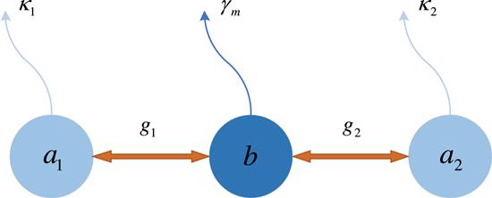
Figure 1. A schematic illustration of a double-cavity optomechanical system: a mechanical mode $b$ in the middle is coupled to two optical cavity modes, ${a}_{1}$ and ${a}_{2},$ which are coupled with each other via phase-dependent phonon-exchange coupling (with the coupling strengths ${g}_{1}$ and ${g}_{2}$). |
In this paper, we adopt another proposal to explore the dynamical evolution of the optomechanical system by inserting periodical modulations into the equation (1 ). Simultaneously, the frequencies of the optical cavities and the mechanical resonator are modulated dynamically, where the modulation term is ${{{\rm H}}}_{M}=\tfrac{1}{2}\xi \nu \,\cos \left(\nu t\right)\left({a}_{1}^{\dagger }{a}_{1}+{a}_{2}^{\dagger }{a}_{2}+{b}^{\dagger }b\right).$ The transformed Hamiltonian of the system in a rotating frame at the driving laser can be obtained:3 )5 ), we can see that the fourth and fifth terms correspond to the beam-splitter interaction and the two-mode squeezing interaction $\left(\left.{G}_{1}\delta {a}_{1}^{\dagger }\delta {b}^{\dagger }+{G}_{1}^{* }\delta {a}_{1}\delta b\right)-\left({G}_{2}\delta {a}_{2}^{\dagger }\delta {b}^{\dagger }+{G}_{2}^{* }\delta {a}_{2}\delta b\right.\right).$ Taking advantage of this feature, whereby the beam-splitter interaction has the energy exchange between the photon state and the phonon state, the number of thermal phonons can be reduced to achieve ground-state cooling. The environmental thermal phonon number is defined by ${n}_{{\rm{th}}}=1/\left[\exp \left(\hslash {\omega }_{m}/{k}_{{\rm{B}}}T\right)-1\right],$ where ${k}_{{\rm{B}}}$ is the Boltzmann constant and $T$ is the environmental temperature. Therefore, the beam-splitter interaction usually becomes an important prerequisite for strengthening the anti-Stokes or suppressing the Stokes processes in sideband cooling mechanisms. At the same time, we also need to strictly meet the requirements of small cavity decay and weak optomechanical coupling strength, and the FM added later can ably overcome these restrictions. It is necessary to study the system dynamics $\left({G}_{1}{\delta }{a}_{1}^{\dagger }{\delta }b+{G}_{1}^{* }{\delta }{a}_{1}{\delta }{b}^{\dagger }-{G}_{2}{\delta }{a}_{2}^{\dagger }{\delta }b-{G}_{2}^{* }{\delta }{a}_{2}{\delta }{b}^{\dagger }\right)$ by fully understanding the effect of the free term FM in equation (5 ). Therefore, we firstly apply the following transformation decomposition term:8 ). The transformed Hamiltonian can be rewritten as
$\begin{eqnarray}\begin{array}{l}H^{\prime} ={{\rm{\Delta }}}_{1}{a}_{1}^{\dagger }{a}_{1}+{{\rm{\Delta }}}_{2}{a}_{2}^{\dagger }{a}_{2}+{\omega }_{m}{b}^{\dagger }b\\ \,+\left({g}_{1}{a}_{1}^{\dagger }{a}_{1}-{g}_{2}{a}_{2}^{\dagger }{a}_{2}\right)\left(b+{b}^{\dagger }\right)+{{\rm{\Omega }}}_{1}\left({a}_{1}+{a}_{1}^{\dagger }\right)\\ \,+{{\rm{\Omega }}}_{2}\left({a}_{2}+{a}_{2}^{\dagger }\right)+\displaystyle \frac{1}{2}\xi \nu \,\cos \left(\nu t\right)\left({a}_{1}^{\dagger }{a}_{1}+{a}_{1}^{\dagger }{a}_{2}+{b}^{\dagger }b\right),\end{array}\end{eqnarray}$
where ${{\rm{\Delta }}}_{i}={\omega }_{i}-{\omega }_{{\rm{Li}}}\left(i=1,2\right)$ is the double-cavity mode detuning with the corresponding external driving laser. For convenience, it can be assumed that the frequencies of the two control fields are equal, which is ${\omega }_{L1}=\omega {}_{L2}={\omega }_{c}.$ Here, $\xi $ is the normalized modulation amplitude and $\nu $ is the modulation frequency. Taking all the damping processes and noise effects into account, the following nonlinear quantum Langevin equations can be obtained based on equation ( $\begin{eqnarray}\begin{array}{l}{\dot{a}}_{1}=-\left({\rm{i}}{{\rm{\Delta }}}_{1}+\displaystyle \frac{{\kappa }_{1}}{2}\right){a}_{1}-{\rm{i}}{g}_{1}{a}_{1}\left(b+{b}^{\dagger }\right)\\ \,-{\rm{i}}\displaystyle \frac{1}{2}\xi \nu \,\cos \left(\nu t\right){a}_{1}-{\rm{i}}{{\rm{\Omega }}}_{1}-\sqrt{{\kappa }_{1}}{a}_{1,{\rm{in}}},\\ {\dot{a}}_{2}=-\left({\rm{i}}{{\rm{\Delta }}}_{2}+\displaystyle \frac{{\kappa }_{2}}{2}\right){a}_{2}+{\rm{i}}{g}_{2}{a}_{2}\left(b+{b}^{\dagger }\right)\\ \,-{\rm{i}}\displaystyle \frac{1}{2}\xi \nu \,\cos \left(\nu t\right){a}_{2}-{\rm{i}}{{\rm{\Omega }}}_{2}-\sqrt{{\kappa }_{2}}{a}_{2,{\rm{in}}},\\ \dot{b}=-\left({\rm{i}}{\omega }_{m}+\displaystyle \frac{{\gamma }_{m}}{2}\right)b-{\rm{i}}{g}_{1}{a}_{1}^{\dagger }{a}_{1}+{\rm{i}}{g}_{2}{a}_{2}^{\dagger }{a}_{2}\\ \,-{\rm{i}}\displaystyle \frac{1}{2}\xi \nu \,\cos \left(\nu t\right)b-\sqrt{{\gamma }_{m}}{b}_{{\rm{in}}},\end{array}\end{eqnarray}$
where ${\kappa }_{i}$ and ${\gamma }_{m}$ represent the damping rates of the cavity mode ${a}_{i},$ and the mechanical mode, respectively. Moreover, the corresponding noise operators ${a}_{i,{\rm{in}}}$ and ${b}_{{\rm{in}}}$ satisfy the correlation $\left\langle {a}_{i,{\rm{in}}}\right\rangle =\left\langle {b}_{{\rm{in}}}\right\rangle =0$ under strongly coherent laser driving. After the linearization, the new Hamiltonian at the input laser frequency ${\omega }_{c}$ can be simplified as: $\begin{eqnarray}\begin{array}{l}{H}_{{\rm{L}}\,{\rm{F}}}={{\rm{\Delta }}^{\prime} }_{1}\delta {a}_{1}^{\dagger }\delta {a}_{1}+{{\rm{\Delta }}^{\prime} }_{2}\delta {a}_{2}^{\dagger }\delta {a}_{2}+{\omega }_{m}\delta {b}^{\dagger }\delta b\\ \,+\left({G}_{1}\delta {a}_{1}^{\dagger }+{G}_{1}^{* }\delta {a}_{1}\right)\left(\delta b+\delta {b}^{\dagger }\right)\\ \,-\left({G}_{2}\delta {a}_{2}^{\dagger }+{G}_{2}^{* }\delta {a}_{2}\right)\left(\delta b+\delta {b}^{\dagger }\right)\\ \,+\displaystyle \frac{1}{2}\xi \nu \,\cos \left(\nu t\right)\left(\delta {a}_{1}^{\dagger }\delta {a}_{1}+\delta {a}_{2}^{\dagger }\delta {a}_{2}+\delta {b}^{\dagger }\delta b\right),\end{array}\end{eqnarray}$
where ${{\rm{\Delta }}^{\prime} }_{i}={{\rm{\Delta }}}_{i}-{g}_{i}\left(\beta +{\beta }^{* }\right)(i=1,2)$ describes the detuning modified by optomechanical coupling, and ${G}_{i}={\alpha }_{i}{g}_{i}(i\,=1,2)$ denotes the linearized coupling strength between the cavity mode ${a}_{i}$ and mechanical mode $b.$ Based on equation ( $\begin{eqnarray}{V}_{0}={V}_{01}+{V}_{02}+{V}_{03},\end{eqnarray}$
where $\begin{eqnarray}\begin{array}{l}{V}_{01}={T}\exp \left\{-{\rm{i}}\displaystyle {\int }_{0}^{t}{\rm{d}}\tau \left({{\rm{\Delta }}}_{1}\delta {a}_{1}^{\dagger }\delta {a}_{1}+{{\rm{\Delta }}}_{2}\delta {a}_{2}^{\dagger }\delta {a}_{2}\right)\right\}\\ \,=\exp \left\{-{\rm{i}}{{{\rm{\Delta }}}_{1}}^{^{\prime} }t\left(\delta {a}_{1}^{\dagger }\delta {a}_{1}\right)-{\rm{i}}{{{\rm{\Delta }}}_{2}}^{^{\prime} }t\left(\delta {a}_{2}^{\dagger }\delta {a}_{2}\right)\right\},\\ {V}_{02}={T}\exp \left\{-{\rm{i}}\displaystyle {\int }_{0}^{t}{\rm{d}}\tau \left({\omega }_{m}\delta {b}^{\dagger }\delta b\right)\right\}\\ \,=\exp \left\{-{\rm{i}}{\omega }_{m}t\left(\delta {b}^{\dagger }\delta b\right)\right\},\\ {V}_{03}={T}\exp \left\{-{\rm{i}}\displaystyle {\int }_{0}^{t}{\rm{d}}\tau \left(\displaystyle \frac{1}{2}\xi \nu \,\cos \left(\nu t\right)\right.\right.\\ \,\times \left.\left.\left(\delta {a}_{1}^{\dagger }\delta {a}_{1}-\delta {a}_{2}^{\dagger }\delta {a}_{2}+\delta {b}^{\dagger }\delta b\right)\right)\Space{0ex}{3ex}{0ex}\right\}\\ \,=\exp \left\{-\displaystyle \frac{{\rm{i}}}{2}\xi \,\sin \left(\nu t\right)\left(\delta {a}_{1}^{\dagger }\delta {a}_{1}+\delta {a}_{2}^{\dagger }\delta {a}_{2}+\delta {b}^{\dagger }\delta b\right)\right\},\end{array}\end{eqnarray}$
where ${T}$ represents the time ordering operator. Moreover, by applying the unitary transformation ${\tilde{H}}_{{\rm{LF}}}\to {{V}_{0}}^{\dagger }{H}_{{\rm{LF}}}{V}_{0}-{\rm{i}}{{V}_{0}}^{\dagger }{\dot{V}}_{0}$ to the interaction picture, the corresponding Hamiltonian takes the form $\begin{eqnarray}\begin{array}{l}{\tilde{H}}_{{\rm{LF}}}={G}_{1}\left(\delta {a}_{1}^{\dagger }\delta {b}^{\dagger }{{\rm{e}}}^{{\rm{i}}[\left({{\rm{\Delta }}^{\prime} }_{1}+{\omega }_{m}\right)t+\xi \,\sin \left(\nu t\right)]}\right.\\ \,+\left.\delta {a}_{1}^{\dagger }\delta b{{\rm{e}}}^{{\rm{i}}\left({{\rm{\Delta }}^{\prime} }_{1}-{\omega }_{m}\right)t}\right)\\ \,-{G}_{2}\left(\delta {a}_{2}^{\dagger }\delta {b}^{\dagger }{{\rm{e}}}^{{\rm{i}}[\left({{\rm{\Delta }}^{\prime} }_{2}+{\omega }_{m}\right)t+\xi \,\sin \left(\nu t\right)]}+\delta {a}_{2}^{\dagger }\delta b{{\rm{e}}}^{{\rm{i}}\left({{\rm{\Delta }}^{\prime} }_{2}-{\omega }_{m}\right)t}\right)\\ \,+{{\rm{{\rm H}}}}_{\cdot }{{\rm{c}}}_{\cdot },\end{array}\end{eqnarray}$
in which we use the Jacobi–Anger expansions ${{\rm{e}}}^{{\rm{i}}\xi \,\sin \left(\nu t\right)}=\displaystyle {\sum }_{k=-\propto }^{\propto }{{\rm{J}}}_{k}\left(\xi \right){e}^{ik\nu t}$ in equation ( $\begin{eqnarray}\begin{array}{l}{\tilde{H}}_{{\rm{LF}}}={G}_{1}\delta {a}_{1}^{\dagger }\delta b{{\rm{e}}}^{{\rm{i}}\left({{\rm{\Delta }}^{\prime} }_{1}-{\omega }_{m}\right)t}-{G}_{2}\delta {a}_{2}^{\dagger }\delta b{{\rm{e}}}^{{\rm{i}}\left({{\rm{\Delta }}^{\prime} }_{2}-{\omega }_{m}\right)t}\\ \,+\displaystyle \sum _{k=-\infty }^{\infty }{G}_{1}{{\rm{J}}}_{k}\left(\xi \right)\delta {a}_{1}^{\dagger }\delta {b}^{\dagger }{{\rm{e}}}^{{\rm{i}}\left({{\rm{\Delta }}^{\prime} }_{1}+{\omega }_{m}+k\nu \right)t}\\ \,-\displaystyle \sum _{k=-\infty }^{\infty }{G}_{2}{{\rm{J}}}_{k}\left(\xi \right)\delta {a}_{2}^{\dagger }\delta {b}^{\dagger }{{\rm{e}}}^{{\rm{i}}\left({{\rm{\Delta }}^{\prime} }_{2}+{\omega }_{m}+k\nu \right)t}+{{\rm{{\rm H}}}}_{\cdot }{{\rm{c}}}_{\cdot },\end{array}\end{eqnarray}$
where ${{\rm{J}}}_{k}\left(\xi \right)$ is the first kind of Bessel function with kth order, and $k$ is an integer. To better learn how to significantly improve the cooling of the mechanical resonator via the FM proposal, a good solution can be obtained by dissecting the physics process with the energy levels of the total system in the displaced frame. We set the red-detuning sideband conditions ${{\rm{\Delta }}^{\prime} }_{1}={{\rm{\Delta }}^{\prime} }_{2}={\omega }_{m}.$ The anti-Stokes processes (beam-splitter interaction) are on resonant, to improve the mechanical cooling processes. It is worth noting that the Stokes processes differ markedly from the former. Due to the existence of the detuning $\left(2{\omega }_{m}+k\nu \right)$ with the coupling strength ${G}_{1}{{\rm{J}}}_{k}\left(\xi \right)$ and ${G}_{2}{{\rm{J}}}_{k}\left(\xi \right),$ the Stokes processes can be modulated individually and effectively by selecting the appropriate parameters $\xi $ and $\nu .$ Therefore, we can observe that the heating processes will be strongly suppressed if the ratio ${G}_{i=1,2}{{\rm{J}}}_{k}\left(\xi \right)/\left(2{\omega }_{m}+k\nu \right)$ can be decreased notably by modulating the aforementioned two parameters properly.Another approach to understanding the modulation mechanism involves utilizing the properties of the Bessel function. It is well known that the Stokes heating processes may take place at any time, and any two contiguous heating processes are separated by modulation frequency $\nu $ space. Given a fixed value $\nu ,$ the ratio ${G}_{i=1,2}{{\rm{J}}}_{k}\left(\xi \right)/\left(2{\omega }_{m}+k\nu \right)$ of resonant sidebands can be reduced as much as possible by choosing an appropriate parameter $\xi .$ This takes advantage of the characteristics whereby there are always parameters $\xi $ satisfied ${{\rm{J}}}_{{k}_{0}}\left(\xi \right)=0$ in the Bessel function, as illustrated in figure 2. Furthermore, the modulation frequency $\nu $ is proportional to the number of Stokes processes. A larger modulation frequency can effectively reduce the occurrence of Stokes processes within the bandwidth. Therefore, the heating effects of Stokes processes far away from the bandwidth of the optical cavity in the mechanical motion can be ignored. Nevertheless, the ratio ${G}_{1,2}/2{\omega }_{m}$ will be a constant if FM is not applied to the system, which means that the effective mechanical cooling needs to meet the constraint ${G}_{1,2}\gg 2{\omega }_{m}$ to suppress the Stokes heating process. It is also the primary restriction of the cooling of the mechanical resonator under normal sideband conditions.
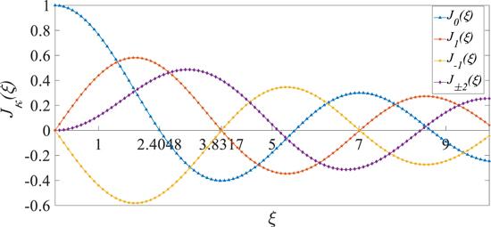
Figure 2. The value of the Bessel function of the first kind ${J}_{k}\left(\xi \right)$ with different normalized modulation amplitudes. |
In summary, the FM approach plays a crucial role in the control of system parameters to suppress the Stokes heating processes. It means that these advances will provide a new pathway to break the limits of cavity optomechanical cooling.
3. Stability conditions
To obtain the cooling effect of the mechanical resonator, we will work on the mean phonon number of the steady-state region in the mechanical mode. We consider that each operator in equation (4 ) can be rewritten in terms of the classical mean value part and the quantum fluctuation part in the strong driving regime, namely, ${a}_{1}={\alpha }_{1}+\delta {a}_{1},$ ${a}_{2}={\alpha }_{2}+\delta {a}_{2},$ $b=\beta +\delta b.$ The mean values, ignoring the inherent noise terms, can be expressed as:
$\begin{eqnarray}\begin{array}{l}{\dot{\alpha }}_{1}=-\left[{\rm{i}}{{\rm{\Delta }}^{\prime} }_{1}+\displaystyle \frac{{\kappa }_{1}}{2}\right]{\alpha }_{1}-{\rm{i}}\displaystyle \frac{1}{2}\xi \nu \,\cos \left(\nu t\right){\alpha }_{1}-{\rm{i}}{{\rm{\Omega }}}_{1},\\ {\dot{\alpha }}_{2}=-\left[{\rm{i}}{{\rm{\Delta }}^{\prime} }_{2}+\displaystyle \frac{{\kappa }_{2}}{2}\right]{\alpha }_{2}-{\rm{i}}\displaystyle \frac{1}{2}\xi \nu \,\cos \left(\nu t\right){\alpha }_{2}-{\rm{i}}{{\rm{\Omega }}}_{2},\\ \dot{\beta }=-\left[{\rm{i}}{\omega }_{m}+\displaystyle \frac{{\gamma }_{m}}{2}\right]\beta -{\rm{i}}\displaystyle \frac{1}{2}\xi \nu \,\cos \left(\nu t\right)\beta \\ \,-{\rm{i}}\left({g}_{1}{\left|{\alpha }_{1}\right|}^{2}+{g}_{2}{\left|{\alpha }_{2}\right|}^{2}\right).\end{array}\end{eqnarray}$
Next, ignoring the nonlinear terms, the other form for the linearized quantum fluctuations can be obtained:11 ) with the quadrature forms of the cavity modes and the analogous Hermitian input noises, i.e. $\delta {\nu }_{o={a}_{1},{a}_{2},b}=\left(\delta o-\delta {o}^{\dagger }\right)/{\rm{i}}\sqrt{2},$ $\delta {u}_{o={a}_{1},{a}_{2},b}=\left(\delta o+\delta {o}^{\dagger }\right)/\sqrt{2},$ and ${u}_{o={a}_{1},{a}_{2},b}^{{\rm{in}}}=\left({o}_{{\rm{in}}}+{o}_{{\rm{in}}}^{\dagger }\right)/\sqrt{2},$ ${v}_{o={a}_{1},{a}_{2},b}^{{\rm{in}}}=\left({o}_{{\rm{in}}}-{o}_{{\rm{in}}}^{\dagger }\right)/{\rm{i}}\sqrt{2}.$ Now, the steady-state expected values of the phonon number operators can be rewritten with the matrix form
$\begin{eqnarray}\begin{array}{l}\delta {\dot{a}}_{1}=-\left[{\rm{i}}{{\rm{\Delta }}^{\prime} }_{1}+\displaystyle \frac{{\kappa }_{1}}{2}\right]\delta {a}_{1}-{\rm{i}}\displaystyle \frac{1}{2}\xi \nu \,\cos \left(\nu t\right)\delta {a}_{1}\\ \,-{\rm{i}}{G}_{1}\left(\delta b+\delta {b}^{\dagger }\right)-\sqrt{{\kappa }_{1}}{a}_{1,{\rm{in}}},\\ \,\delta {\dot{a}}_{2}=-\left[{\rm{i}}{{\rm{\Delta }}^{\prime} }_{2}+\displaystyle \frac{{\kappa }_{2}}{2}\right]\delta {a}_{2}-{\rm{i}}\displaystyle \frac{1}{2}\xi \nu \,\cos \left(\nu t\right)\delta {a}_{2}\\ \,+{\rm{i}}{G}_{2}\left(\delta b+\delta {b}^{\dagger }\right)-\sqrt{{\kappa }_{2}}{a}_{2,\mathrm{in}},\\ \,\delta \dot{b}=-\left[{\rm{i}}{\omega }_{m}+\displaystyle \frac{{\gamma }_{m}}{2}\right]\delta b-{\rm{i}}\displaystyle \frac{1}{2}\xi \nu \,\cos \left(\nu t\right)\delta b\\ \,-{\rm{i}}{G}_{1}\delta {a}_{1}^{\dagger }-{\rm{i}}{G}_{1}^{* }\delta {a}_{1}+{\rm{i}}{G}_{2}\delta {a}_{2}^{\dagger }+{\rm{i}}{G}_{2}^{* }\delta {a}_{2}\\ \,-\sqrt{{\gamma }_{m}}{b}_{{\rm{in}}}{\rm{.}}\end{array}\end{eqnarray}$
Here, we have neglected the nonlinear terms ${\rm{i}}g{\delta }{a}_{1}\left({\delta }{b}^{\dagger }+{\delta }b\right),$ ${\rm{i}}g\delta {a}_{2}\left(\delta {b}^{\dagger }+\delta b\right)$, and ${\rm{i}}{g}_{1}\delta {a}_{1}\delta {a}_{1}^{\dagger },$ ${\rm{i}}{g}_{2}\delta {a}_{2}\delta {a}_{2}^{\dagger }$ under the strong coherent laser driving. We substitute these operators in equation ( $\begin{eqnarray}\dot{{\boldsymbol{f}}}\left(t\right)={\boldsymbol{A}}{\boldsymbol{f}}\left(t\right)+{\boldsymbol{C}}\left(t\right),\end{eqnarray}$
where ${\boldsymbol{f}}\left({\boldsymbol{t}}\right)$ is the matrix-vector of the fluctuations and ${\boldsymbol{C}}\left(t\right)$ is the matrix-vector of the noise sources. Their forms are defined by $\begin{eqnarray}\begin{array}{l}{\boldsymbol{f}}{\left(t\right)}^{{\rm{T}}}=\left(\delta {u}_{{a}_{1}},\delta {\nu }_{{a}_{1}},\delta {u}_{{a}_{2}},\delta {\nu }_{{a}_{2}},\delta {u}_{b},\delta {\nu }_{b}\right),\\ {\boldsymbol{C}}{\left(t\right)}^{{\rm{T}}}=\left(\sqrt{2{\kappa }_{1}}{u}_{{a}_{1}}^{{\rm{in}}},\sqrt{2{\kappa }_{1}}{v}_{{a}_{1}}^{{\rm{in}}},\sqrt{2{\kappa }_{2}}{u}_{{a}_{2}}^{{\rm{in}}},\right.\\ \,\times \left.\sqrt{2{\kappa }_{2}}{v}_{{a}_{2}}^{{\rm{in}}},\sqrt{2{\gamma }_{m}}{u}_{b}^{{\rm{in}}},\sqrt{2{\gamma }_{m}}{v}_{b}^{{\rm{in}}}\right),\end{array}\end{eqnarray}$
and the corresponding transformation matrix is given by $\begin{eqnarray}{\boldsymbol{A}}=\left(\begin{array}{llllll}-\displaystyle \frac{{\kappa }_{1}}{2} & {D}_{1} & 0 & 0 & 0 & 0\\ -{D}_{1} & -\displaystyle \frac{{\kappa }_{1}}{2} & 0 & 0 & -2{G}_{1} & 0\\ 0 & 0 & -\displaystyle \frac{{\kappa }_{2}}{2} & {D}_{2} & 0 & 0\\ 0 & 0 & -{D}_{2} & -\displaystyle \frac{{\kappa }_{2}}{2} & 2{G}_{2} & 0\\ 0 & 0 & 0 & 0 & -\displaystyle \frac{{\gamma }_{m}}{2} & {D}_{3}\\ -2{G}_{1} & 0 & 2{G}_{2} & 0 & -{D}_{3} & -\displaystyle \frac{{\gamma }_{m}}{2}\end{array}\right),\end{eqnarray}$
where ${D}_{1}={{\rm{\Delta }}^{\prime} }_{1}+\tfrac{1}{2}\xi \nu \,\cos \left(\nu t\right),$ ${D}_{2}={{\rm{\Delta }}^{\prime} }_{2}+\tfrac{1}{2}\xi \nu \,\cos \left(\nu t\right),$ ${{\rm{\Omega }}}_{m}={\omega }_{m}+\tfrac{1}{2}\xi \nu \,\cos \left(\nu t\right)$ are the renormalized parameters.The stability of the system is satisfied only if all the eigenvalues of the drift matrix ${\boldsymbol{A}}$ are negative. The stability conditions can be explicitly given by the Routh–Hurwitz criterion [59]. In this case, we specifically plot the stability as a function of the optomechanical coupling strength ${G}_{2}$ and the other coupling strength ${G}_{1}$ by applying it to calculate the matrix ${\boldsymbol{A}}$, as shown in figure 3. The stable region and unstable region are denoted by the blue and yellow areas, respectively. The red dotted line represents the boundary between the stable and unstable regions. Furthermore, the parameters of the system we study are ${{\rm{\Delta }}^{\prime} }_{1}={{\rm{\Delta }}^{\prime} }_{2}={\omega }_{m},$ ${\kappa }_{1}={\kappa }_{2}=0.1{\omega }_{m},$ ${\gamma }_{m}={10}^{-5}{\omega }_{m},$ $\xi =0,$ $\nu =0.$
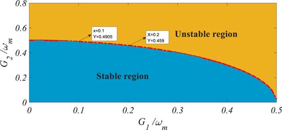
Figure 3. The dynamical stability region for the double-cavity optomechanical system in the absence of FM, in which ${G}_{2}$ is a function of ${G}_{1},$ and the other parameters are ${{\rm{\Delta }}^{\prime} }_{1}={{\rm{\Delta }}^{\prime} }_{2}={\omega }_{m},$ ${\kappa }_{1}={\kappa }_{2}=0.1{\omega }_{m},$ ${\gamma }_{m}={10}^{-5}{\omega }_{m},$ $\xi =0,$ $\nu =0.$ |
In the following considerations, we are dedicated to the exploration of cooling the mechanical resonator with FM in different sideband conditions, and all the given parameters are selected from the stable region to the unstable region.
4. Quantum master equation and numerical simulation
To visualize the dynamics of the mechanical resonator of the optomechanical system, we employ the quantum master equation approach to obtain the numerical simulation for the mean phonon number starting from the linearized Hamiltonian. The evolution of the system density matrix $\rho $ can be governed by the following quantum master equationappendix . Furthermore, we focus on the time evolution of the mean phonon numbers of the mechanical resonator, that is ${\bar{N}}_{b}=\left\langle {b}^{\dagger }b\right\rangle ={\rm{Tr}}\left({b}^{\dagger }b\rho \right).$ To solve the numerical simulation of the mean phonon number, we generally assume that the initial state of the system, where only the mechanical mode is occupied, i.e. $\left\langle {b}^{\dagger }b\right\rangle \left(t=0\right)={n}_{{\rm{th}}}.$ Other second-order moments disappear and assign them to zero. The exact results of the second-order correlation function can be obtained numerically by calculating these ordinary differential equations from equation (16 ).
$\begin{eqnarray}\dot{\rho }={\rm{i}}\left[\rho ,{{{\rm H}}}_{{\rm{LF}}}\right]+{L}_{a1}\left[\rho \right]+{L}_{a2}\left[\rho \right]+{L}_{b}\left[\rho \right],\end{eqnarray}$
where ${L}_{a1}\left[\rho \right]=\tfrac{{\kappa }_{1}}{2}\left(2{a}_{1}\rho {a}_{1}^{\dagger }-{a}_{1}^{\dagger }{a}_{1}\rho -\rho {a}_{1}^{\dagger }{a}_{1}\right),{L}_{a2}\left[\rho \right]\,=$ $\tfrac{{\kappa }_{2}}{2}\left(2{a}_{2}\rho {a}_{2}^{\dagger }\,-{a}_{2}^{\dagger }{a}_{2}\rho -\rho {a}_{2}^{\dagger }{a}_{2}\right),$ and ${L}_{b}\left[{\rho }\right]=\tfrac{{{\gamma }}_{m}}{2}\left({n}_{{\rm{t}}{\rm{h}}}+1\right)\left(2{b}_{1}{\rho }{b}_{1}^{\dagger }-{b}_{1}^{\dagger }{b}_{1}{\rho }\,-{\rho }{b}_{1}^{\dagger }{b}_{1}\right)+\tfrac{{{\gamma }}_{m}}{2}\left(2{b}_{1}^{\dagger }{\rho }{b}_{1}-{b}_{1}{b}_{1}^{\dagger }{\rho }-{\rho }{b}_{1}{b}_{1}^{\dagger }\right).$ Based on the above total master equation, we can obtain the equations of motion $\begin{eqnarray}\dot{{\boldsymbol{V}}}={\boldsymbol{M}}{\boldsymbol{V}}+{\boldsymbol{N}},\end{eqnarray}$
where ${\boldsymbol{V}}=$ $\left({\bar{N}}_{{a}_{1}}\right.,$ ${\bar{N}}_{{a}_{2}},$ ${\bar{N}}_{b},$ $\left\langle {a}_{1}{a}_{2}\right\rangle ,$ $ \langle {a}_{1}^{\dagger }{a}_{2}^{\dagger } \rangle ,$ $\left\langle {a}_{1}{a}_{2}^{\dagger }\right\rangle ,$ $\left\langle {a}_{1}^{\dagger }{a}_{2}\right\rangle ,$ $\left\langle {a}_{1}b\right\rangle ,$ $\left\langle {a}_{1}^{\dagger }{b}^{\dagger }\right\rangle ,$ $\left\langle {a}_{1}{b}^{\dagger }\right\rangle ,$ $\left\langle {a}_{1}^{\dagger }b\right\rangle ,$ $\left\langle {a}_{2}b\right\rangle ,$ $ \langle {a}_{2}^{\dagger }{b}^{\dagger } \rangle ,$ $\left\langle {a}_{2}{b}^{\dagger }\right\rangle ,$ $\left\langle {a}_{2}^{\dagger }b\right\rangle ,$ $\left\langle {{a}_{1}}^{2}\right\rangle ,$ $\left\langle {a}_{1}^{\dagger 2}\right\rangle ,$ $\left\langle {{a}_{2}}^{2}\right\rangle ,$ $\left\langle {a}_{2}^{\dagger 2}\right\rangle ,$ $\left\langle {b}^{2}\right\rangle ,$ ${\left.\left\langle {b}^{\dagger 2}\right\rangle \right)}^{{\rm{T}}},$ ${\boldsymbol{N}}=$ $\left(0,\right.$ $0,$ ${\gamma }_{m}{n}_{{\rm{th}}},$ $0,$ $0,$ $0,$ $0,$ $-{\rm{i}}{G}_{1},$ ${\rm{i}}{G}_{1},$ $0,$ $0,$ ${\rm{i}}{G}_{2},$ $-{\rm{i}}{G}_{2},$ $0,$ $0,$ $0,$ $0,$ $0,$ $0,$ $0,$ ${\left.0\right)}^{{\rm{T}}};$ ${\boldsymbol{{\rm M}}}$ is the 21 dimensions drift matrix. It is unnecessary to calculate all the elements of the density operator due to the fact that most of the mean values of the second-order moments can find their conjugate terms. Also, the matrix elements that need to be calculated are presented in the 4.1. Resolved-sideband cooling
Based on the above calculation results, we are now interested in the discussion of the ground-state cooling of the double-cavity optomechanical system in the resolved-sideband regime ${\kappa }_{i}\lt {\omega }_{m}\left(i=1,2\right).$ Here, we choose the red sideband detuning ${{\rm{\Delta }}^{\prime} }_{i}={\omega }_{m}\left(i=1,2\right).$
4.1.1. Weak coupling regime
In this section, we will study the cooling dynamics of the mechanical resonator in the weak coupling regime $\left|{G}_{i}\right|\ll {\kappa }_{i}\left(i=1,2\right).$ Firstly, a comparison of the mean phonon number between the current double-cavity optomechanical system and the conventional single-cavity optomechanical system [46] is shown in figure 4. We plot the mean phonon number for different coupling strengths ${G}_{2}$ in the case of ${G}_{1}=0.01{\omega }_{m}.$ It is evident that the final mean phonon number in the double-cavity system is markedly lower than a single-cavity in weak coupling. In our coupled cavity system, the mechanical resonator can be effectively cooled to the ground state since the Stokes heating processes can be suppressed by the double cooling channel in our current scheme. In figures 5(a) and (b), we compare the time evolution of the mean phonon number with FM or without corresponding to different system parameters. It can show that the cooling effect has not been significantly improved, even with FM in figure 5(a). At this time, the superiority of FM is not obvious due to the fact that the Stokes heating processes themselves have been greatly suppressed in the case of too small cavity decay rates and coupling strengths. However, with the further increase in the cavity decay rates and optical coupling strengths in the same weak coupling region, i.e. ${\kappa }_{1}={\kappa }_{2}=0.2{\omega }_{m},$ ${G}_{1}={G}_{2}=0.1{\omega }_{m},$ the mean phonon number can be reduced well with FM compared to without in figure 5(b). The extent of the suppression of the Stokes heating processes will be limited for the larger cavity decay rates and coupling strengths in the traditional optomechanical system. Therefore, the addition of FM can more effectively inhibit the Stokes effect to achieve better cooling of the mechanical resonator to its ground state.
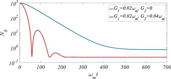
Figure 4. Time evolution of the mean phonon number ${\bar{N}}_{b}$ with FM between the current double-cavity optomechanical system and the conventional single-cavity optomechanical system is plotted for comparison. Other unmentioned parameters are assumed as ${{\rm{\Delta }}^{\prime} }_{1}={{\rm{\Delta }}^{\prime} }_{2}={\omega }_{m},$ ${\kappa }_{1}={\kappa }_{2}=0.1{\omega }_{m},$ ${\gamma }_{m}={10}^{-5}{\omega }_{m},$ ${n}_{th}=1000,$ $\nu =10{\omega }_{m}$, and $\xi =\mathrm{2.4048.}$ |
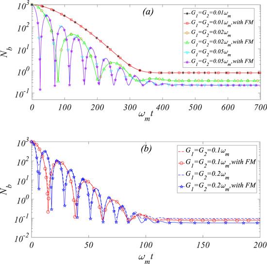
Figure 5. Time evolution of the mean phonon number ${\bar{N}}_{b}$ with or without FM is plotted for comparison: (a) For ${\kappa }_{1}={\kappa }_{2}=0.05{\omega }_{m},$ (b) For ${\kappa }_{1}={\kappa }_{2}=0.2{\omega }_{m}.$ The other parameters are selected to be the same as those in figure 4. |
By combining with the previous analysis, we now provide reasonable conjecture that the effect of FM on the suppression of Stokes heating processes can be significantly improved to achieve better cooling within the range of appropriate parameters.
4.1.2. Strong coupling regime
In contrast to the weak coupling regime, the enhancement of cooling processes can be achieved effectively using the current proposed scheme in the strong coupling regime $G{}_{i}\gg {\kappa }_{i}\left(i=1,2\right).$ We show the dynamical evolution of the mean phonon number with different cavity decay rates in figure 6(a). It is noted that the mean phonon number of the system is significantly lower with the addition of FM than without FM. We also find that the final mean phonon number reduces with the increase in cavity decay rates. Furthermore, the system cooling improvement rate will increase with the increase in the cavity decay rates in the same coupling strengths after data verification. For instance, taken as the three sets of parameters ${\kappa }_{i}/{\omega }_{m}=\left(0.05,0.1,0.15\right)\left(i=1,2\right),$ the final mean phonon number ${\bar{N}}_{b}$ is reduced from 0.261 to 0.206, from 0.147 to 0.102, and from 0.112 to 0.072. The relevant calculation results of the cooling improvement rate are 21.1%, 30.6%, and 35.5%, respectively. It can be interpreted that the superiority of the scheme with FM proposed here becomes more prominent in the strong coupling regime. Furthermore, we also plot the time evolution of the mean phonon number with different coupling strengths ${G}_{2}$ by introducing FM in the unstable region, as shown in figure 6(b). The cooling of the mechanical resonator fails due to the divergent behavior of the phonon number when the coupling strengths are ${G}_{2}/{\omega }_{m}\gt 0.490,$ ${G}_{1}/{\omega }_{m}=0.1{\omega }_{m},$ or ${G}_{2}/{\omega }_{m}\gt 0.459,$ ${G}_{1}/{\omega }_{m}=0.1$ corresponding to the unstable region (see the stability conditions in figure 3). However, the final mean phonon number can be cooled to the quantum ground-state successfully by introducing FM. It is evident that, due to the existence of the FM, the Stokes process can be fully suppressed and better cooling of the mechanical resonator can be achieved than without FM, even in the unstable region.
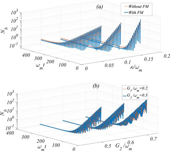
Figure 6. (a) Time evolution of the mean phonon number ${\bar{N}}_{b}$ with or without FM for different optical cavity decay by solving the master equation numerically is plotted for comparison: here, ${G}_{1}={G}_{2}=0.2{\omega }_{m}$ and ${\kappa }_{1}={\kappa }_{2}=\kappa .$ (b) Time evolution of the mean phonon number ${\bar{N}}_{b}$ with different coupling strengths in the unstable region. The orange dashed line is for ${G}_{1}/{\omega }_{m}=0.2,$ and the blue solid line represents ${G}_{1}/{\omega }_{m}=\mathrm{0.3.}$ The other parameters are selected to be the same as those in figure 4. |
4.2. Unresolved-sideband cooling
We have already discussed the cooling of the resolved-sideband regime in the stable region. In this section, we now explore how to achieve a better cooling effect by optimizing the FM even in the unresolved-sideband regime. Figure 7 shows the dynamical evolution of the mean phonon number with different cavity decay rates in ${G}_{1}={G}_{2}=0.2{\omega }_{m}.$ The cooling effect in the presence of the FM is dramatically improved compared to the conventional double-cavity system. The results indicate that the former cooling limit is much lower than without FM in the stable region. We also note that the mean phonon number cannot be lower than unity for the large cavity decay rate. This is because overlarge cavity decay rates limit the final cooling of the mechanical resonator. Apart from the saturation effect of the cooling rate, the reason for this phenomenon is that the anti-Stokes effect becomes weaker. However, the mean phonon number successfully reaches the ground-state cooling by making use of the FM. This can be interpreted as that FM makes a major contribution to the suppression of the Stokes heating processes, which will be very beneficial to the ground-state cooling experiments of mechanical resonators, even in the unresolved-sideband regime.
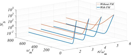
Figure 7. Time evolution of the mean phonon number ${N}_{b}$ corresponding to different cavity decay rates with or without FM. Here, ${G}_{1}={G}_{2}=0.2{\omega }_{m}.$ The other parameters are selected to be the same as those in figure 4. |
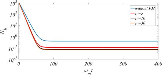
Combining the results of figure 7, we make a reasonable guess that a possible way to achieve a better cooling result is to have a larger frequency of the modulation term in equation (5 ). In figure 8, the cooling dynamics for different modulation frequencies are depicted with solid curves in different colors. The mechanical resonators have good cooling efficiency when we choose the system parameters ${\kappa }_{1}={\kappa }_{2}=2{\omega }_{m},$ ${G}_{1}={G}_{2}=0.2{\omega }_{m}.$ It is noteworthy that the corresponding cooling efficiency is improved as the modulation frequency increases. Nevertheless, the final mean phonon number is almost no different when the modulation frequencies are large enough when $\nu =10$ and $\nu =30.$ The results demonstrate that a too large modulation frequency is confirmed to be of little practical feasibility to the improvement of mechanical cooling results. The Stokes heating process far from the resonant conditions has little effect on the cooling process when the modulation frequency is large enough, or even negligible. It can be explained by a frequency-domain interpretation of optomechanical interactions [46]. Therefore, it is particularly crucial to choose a suitable rather than an overlarge modulation frequency to obtain a better cooling effect.
Figure 8. Time evolution of the mean phonon number ${N}_{b}$ for different modulation frequencies by solving the master equation numerically is plotted for comparison. Here, ${\kappa }_{1}={\kappa }_{2}=2{\omega }_{m},$ ${G}_{1}={G}_{2}=0.2{\omega }_{m}.$ The other parameters are selected to be the same as those in figure 4. |
5. Conclusion
In summary, we have used the double-cavity optomechanical system as an example to study the ground-state cooling of a mechanical resonator by solving quantum master equations and employing the covariance approach. In this work, we have theoretically proposed an FM scheme for improving the ground-state cooling of the mechanical resonator from the stable to the unstable region, from the resolved-sideband regime to the unresolved-sideband regime. It is demonstrated by numerical simulations that, in our current scheme, the mechanical resonator can be cooled to its ground-state with a lower limit than in the conventional double-cavity optomechanical system due to the suppression of the Stokes heating processes. In the commonly concerned dynamically stable regime, we have discussed and analyzed the comparison between the time evolutions of the mean phonon number in the weak coupling regime and the strong coupling regime with FM or without. Moreover, in the presence of FM, the final mean phonon number is also well below unity in the unresolved-sideband regime, even if ground-state cooling cannot be achieved in the absence of FM. Finally, we also find that the cooling effect is greatly improved at a higher modulation frequency compared with a lower modulation frequency. The scheme developed in this paper will offer the prospect of the cooling of mechanical resonators, and research and explorations will be richer and more interesting as a result.
Funding
This work was supported by the National Natural Science Foundation of China (Grant No. 62061028), the Foundation for Distinguished Young Scientists of Jiangxi Province (Grant No. 20162BCB23009), the Open Research Fund Program of the State Key Laboratory of Low-Dimensional Quantum Physics (Grant No. KF202010), the Interdisciplinary Innovation Fund of Nanchang University (Grant No. 9166-27060003-YB12), and the Open Research Fund Program of Key Laboratory of Opto-Electronic Information Acquisition and Manipulation of Ministry of Education (Grant No. OEIAM202004).
Appendix. Dynamical equations for the second-order moments
$\begin{eqnarray}\begin{array}{l}\displaystyle \frac{\rm{d}}{\rm{d}t} \bar{N}_{a1}=-{\kappa}_{1}\bar{N}_{a1}+\rm{i}(-{G}_{1}{\langle {a}_{1} b \rangle }^{* }-{G}_{1}{\langle {a}_{1}{b}^{\dagger }\rangle }^{* }\\ +{G}_{1}^{* }\langle {a}_{1}{b}^{\dagger }\rangle +{G}_{1}^{* }\langle {a}_{1}b \rangle ),\\ \displaystyle \frac{\rm{d}}{\rm{d}t} \bar{N}_{a2}=-{\kappa}_{2}\bar{N}_{a2}+\rm{i}(-{G}_{2}{\langle {a}_{2} b \rangle }^{* }-{G}_{2}{\langle {a}_{2}{b}^{\dagger }\rangle }^{* }\\ +{G}_{2}^{* }\langle {a}_{2}{b}^{\dagger }\rangle +{G}_{2}^{* }\langle {a}_{2}b \rangle ) ,\\ \displaystyle \frac{\rm{d}}{\rm{d}t} \bar{N}_{b}=-{\gamma }_{m}\bar{N}_{b}+{\gamma }_{m}n_{th} +\rm{i}(-{G}_{1}{\langle {a}_{1} b \rangle }^{* }-{G}_{1}{\langle {a}_{1}{b}^{\dagger }\rangle }^{* }\\ -{G}_{1}^{* }{\langle {a}_{1}{b}^{\dagger }\rangle}^{* }+{G}_{1}^{* }\langle {a}_{1}b \rangle + {G}_{2}{\langle {a}_{2}{b}\rangle }^{* }-{G}_{2}{\langle {a}_{2}b ^{\dagger }\rangle}^{*} \\ +{G}_{2}^{* }\langle {a}_{2}{b}^{\dagger }\rangle +{G}_{2}^{* }\langle {a}_{2}b \rangle ), \\ \displaystyle \frac{{\rm{d}}}{{\rm{d}}t}\left\langle {a}_{1}b\right\rangle =\left({\rm{i}}\left(-{D}_{1}-{{\rm{\Omega }}}_{m}\right)-\displaystyle \frac{{\kappa }_{1}+{\gamma }_{m}}{2}\right)\left\langle {a}_{1}b\right\rangle \\ \,+{\rm{i}}\left(-{G}_{1}{\bar{N}}_{{a}_{1}}\right.-{G}_{1}\left\langle {{a}_{1}}^{2}\right\rangle -{G}_{1}{\bar{N}}_{b}-{G}_{1}\left\langle {b}^{2}\right\rangle -{G}_{1}\\ \,+\left.{G}_{2}\left\langle {a}_{1}{a}_{2}^{\dagger }\right\rangle +{G}_{2}^{* }\left\langle {a}_{1}{a}_{2}\right\rangle \right),\\ \displaystyle \frac{{\rm{d}}}{{\rm{d}}t}\left\langle {a}_{1}{b}^{\dagger }\right\rangle =\left({\rm{i}}\left(-{D}_{1}+{{\rm{\Omega }}}_{m}\right)-\displaystyle \frac{{\kappa }_{1}+{\gamma }_{m}}{2}\right)\left\langle {a}_{1}{b}^{\dagger }\right\rangle \\ \,+{\rm{i}}\left(-{G}_{1}\right.{\left\langle {b}^{2}\right\rangle }^{* }+{G}_{1}{\bar{N}}_{{a}_{1}}-{G}_{1}{\bar{N}}_{b}+{{G}_{1}}^{* }\left\langle {{a}_{1}}^{2}\right\rangle \\ \,-\left.{G}_{2}\left\langle {a}_{1}{a}_{2}^{\dagger }\right\rangle +{G}_{2}^{* }\left\langle {a}_{1}{a}_{2}\right\rangle \right),\\ \displaystyle \frac{{\rm{d}}}{{\rm{d}}t}\left\langle {a}_{2}b\right\rangle =\left({\rm{i}}\left(-{D}_{2}-{{\rm{\Omega }}}_{m}\right)-\displaystyle \frac{{\kappa }_{2}+{\gamma }_{m}}{2}\right)\left\langle {a}_{2}b\right\rangle \\ \,+{\rm{i}}{\left(-{G}_{1}\left\langle {a}_{1}{a}_{2}^{\dagger }\right\rangle \right.}^{* }-{G}_{1}^{* }\left\langle {a}_{1}{a}_{2}\right\rangle +{G}_{2}{\bar{N}}_{{a}_{2}}+{G}_{2}{\bar{N}}_{{a}_{2}}\\ \,+\left.{G}_{2}+{G}_{2}\left\langle {b}^{2}\right\rangle +{G}_{2}^{* }\left\langle {{a}_{2}}^{2}\right\rangle \right),\\ \displaystyle \frac{{\rm{d}}}{{\rm{d}}t}\left\langle {a}_{2}{b}^{\dagger }\right\rangle =\left({\rm{i}}\left(-{D}_{2}+{{\rm{\Omega }}}_{m}\right)-\displaystyle \frac{{\kappa }_{2}+{\gamma }_{m}}{2}\right)\left\langle {a}_{2}{b}^{\dagger }\right\rangle \\ \,+{\rm{i}}\left({G}_{1}{\left\langle {a}_{1}{a}_{2}^{\dagger }\right\rangle }^{* }\right.+{G}_{1}^{* }\left\langle {a}_{1}{a}_{2}\right\rangle +{G}_{2}{\left\langle {b}^{2}\right\rangle }^{* }+{G}_{2}{\bar{N}}_{{a}_{2}}\\ \,-\left.{G}_{2}\left\langle {a}_{2}^{\dagger }{a}_{2}\right\rangle -{G}_{2}^{* }\left\langle {{a}_{2}}^{2}\right\rangle \right),\\ \displaystyle \frac{{\rm{d}}}{{\rm{d}}t}\left\langle {{a}_{1}}^{2}\right\rangle =-\left(2{\rm{i}}{D}_{1}+{\kappa }_{1}\right)\left\langle {{a}_{1}}^{2}\right\rangle \\ \,-2{\rm{i}}\left(-{G}_{1}\left\langle {a}_{1}{b}^{\dagger }\right\rangle -{G}_{1}\left\langle {a}_{1}b\right\rangle \right),\\ \displaystyle \frac{{\rm{d}}}{{\rm{d}}t}\left\langle {{a}_{2}}^{2}\right\rangle =-\left(2{\rm{i}}{D}_{2}+{\kappa }_{2}\right)\left\langle {{a}_{2}}^{2}\right\rangle \\ \,+2{\rm{i}}\left(-{G}_{2}\left\langle {a}_{2}{b}^{\dagger }\right\rangle -{G}_{2}\left\langle {a}_{2}b\right\rangle \right),\\ \displaystyle \frac{{\rm{d}}}{{\rm{d}}t}\left\langle {b}^{2}\right\rangle =-\left(2{\rm{i}}{{\rm{\Omega }}}_{m}+{\gamma }_{m}\right)\left\langle {b}^{2}\right\rangle \\ \,+2{\rm{i}}\left(-{G}_{1}{\left\langle {a}_{1}{b}^{\dagger }\right\rangle }^{* }-{G}_{1}\left\langle {a}_{1}b\right\rangle +{G}_{2}\left\langle {a}_{2}^{\dagger }b\right\rangle +{G}_{2}^{* }\left\langle {a}_{2}b\right\rangle \right).\end{array}\end{eqnarray}$