We propose a scheme to realize two-parameter estimation via Bose–Einstein condensates confined in a symmetric triple-well potential. The three-mode NOON state is prepared adiabatically as the initial state. The two parameters to be estimated are the phase differences between the wells. The sensitivity of this estimation scheme is studied by comparing quantum and classical Fisher information matrices. As a result, we find an optimal particle number measurement method. Moreover, the precision of this estimation scheme means that the Heisenberg scaling behaves under the optimal measurement.
Fei Yao, Yi-Mu Du, Haijun Xing, Libin Fu. Two-parameter estimation with three-mode NOON state in a symmetric triple-well potential[J]. Communications in Theoretical Physics, 2022, 74(4): 045103. DOI: 10.1088/1572-9494/ac5efd
1. Introduction
Quantum metrology [1–3] has attracted considerable interest in recent years due to its wide applications in both fundamental sciences and applied technologies. As crucial tools in quantum metrology, the quantum parameter estimation theory [4, 5] and Fisher information provide the theoretical bases for enhancing the precision of parameter estimation with quantum resources. In the previous researches, the single-parameter estimation has been well studied and a series of achievements have been made [6–8], such as gravitational wave detection [9], magnetometry [10–12], atomic clocks [13, 14], and quantum gyroscope [15–17].
Although the single parameter estimation plays a significant role in many applications, it is often necessary to estimate multiple parameters simultaneously in practical problems, e.g. quantum imaging [18–20], waveform estimation [21], measurements of multidimensional fields [22], joint estimation of phase and phase diffusion [23, 24]. Studying the multi-parameter estimation is thus an urgent need for effectively solving the practical parameter estimation problems. It has attracted lots of attention [22–38] in recent years. Most of these works aim to propose a general theory and framework for multi-parameter estimation. Few concrete schemes are proposed for realizing practical high-precision multi-parameter estimations. In this article, we will propose a scheme to estimate multiple parameters simultaneously with Heisenberg scaling sensitivity.
The Bose–Josephson junction, formed by confining Bose–Einstein condensate in the double-well potential (in spatial freedom [39] or internal freedom [40, 41] equivalently) is a well-established model [6, 42–44]. It is widely used in quantum parameter estimation as interferometries for its high controllability [6, 42–44]. Especially in some of the schemes [41, 45–48], one can prepare condensate into the two-mode NOON state [49] (also known as GHZ state [50] and Schrödinger cat state [51]), which can perform single parameter estimation in Heisenberg limit precision. As an extension of the double-well interferometry, we will confine Bose condensate in the symmetrical triple-well potential [52–56] to realize high precision two-parameter estimation.
Our measurement scheme consists of four stages: initialization, parameterization, rotation, and measurement. We prepare the condensate into the three-mode NOON state adiabatically as the initial state. The parameters to be estimated are two-phase differences between the wells caused by the external field. The parameterized state is read via the particle number measurement. In order to study the precision of the measurement scheme, we calculate the quantum Fisher information matrix (QFIM) and classical Fisher information matrix (CFIM) on the two parameters. By comparing the CFIM and QFIM, we find that the measurement rotation time significantly affects the measurement precision, and the optimal rotation time is given. In addition, the result shows that the optimal measurement precision of our scheme can approach the Heisenberg scaling.
The paper is organized as follows. In section 2, the model and basic measurement theory are introduced. In section 3, we give the scheme of estimating two parameters with the triple-well system, including initial state preparation, parameterization, rotation, and measurement. The optimal precision and measurement conditions are given by analyzing the CFIM and QFIM. At last, we summarize this article in section 4.
2. Model and basic theory
In this section, we sketch our scheme. We confine N Bose condensed atoms in a symmetric triple-well system (STWS) [52–56], as seen in figure 1(a). Under the three-mode approximation [52], the Hamiltonian of the condensates reads
with j = (i + 1) mod 3 + 1. The operator ${\hat{a}}_{i}^{\dagger }({\hat{a}}_{i})$ is the bosonic creation (annihilation) operator for atoms in the ground state mode of ith well and ${\hat{n}}_{i}={\hat{a}}_{i}^{\dagger }{\hat{a}}_{i}$ is the corresponding particle number operator. J is the tunneling strength between the wells. It is controllable via adjusting the barriers between the wells. U is the atomic on-site interaction, and U > 0 (U < 0) implies a repulsive (attractive) interaction. It is tunable via the Feshbach resonances [60]. Here, we only consider attractive interaction. In this model, the total atom number $N={\sum }_{i=1}^{3}{n}_{i}$ is conserved. The system state can be expanded on Fock state basis {∣n1, n2, n3⟩}, with ni particle in the ith well, i = 1, 2, 3.
Figure 1. (a) The schematic diagram of a symmetric triple-well trapped Bose condensates. (b) Framework of multi-parameter estimation.
When this STWS is placed into an external field, the ground state energy of ith well (mode ${\hat{a}}_{i}$) experiences an energy shift ${{ \mathcal E }}_{i}$ denoted by the Hamiltonian
$\begin{eqnarray}{\hat{H}}_{p}=\sum _{i}{{ \mathcal E }}_{i}{\hat{a}}_{i}^{\dagger }{\hat{a}}_{i},\end{eqnarray}$
while the tunneling and interactions are both turned off (J = U = 0). Particle in mode ${\hat{a}}_{i}$ will obtain a phase shift ${\phi }_{i}={{ \mathcal E }}_{i}t$ after evolution generated by ${\hat{H}}_{p}$ with time t. Phase differences θ1 = φ1 − φ3 and θ2 = φ2 − φ3 are the parameters we are aiming to estimate.
Before introducing details of our scheme, let us recall the framework of multi-parameter estimation as follows (see figure 1(b)).
i
(i)Initialization: prepare system to the initial state $| \psi {\rangle }_{{\mathfrak{i}}}$.
ii
(ii)Parameterization: the initial state $| \psi {\rangle }_{{\mathfrak{i}}}$ is parameterized to the output state $| \psi ({\boldsymbol{\theta }})\rangle =\hat{{ \mathcal U }}({\boldsymbol{\theta }})| \psi {\rangle }_{{\mathfrak{i}}}$ via a unitary evolution $\hat{{ \mathcal U }}({\boldsymbol{\theta }})$, where θ = (θ1, θ2,…,θd) is a vector parameter. In this article, we set $d=2$.
iii
(iii)Rotation: rotate the output state ∣ψ(θ)⟩ to the measurable final state
(iv)Measurement: perform a set of projective measurements $\{{\hat{{\rm{\Pi }}}}_{{\boldsymbol{n}}}\}$ (n represents the possible result) on the final state $| \psi {\rangle }_{{\mathfrak{f}}}$. The probability of observing the result n, which when conditioned to the vector parameter θ, is
Vector θ is estimated based on {Pn}, statistics of the measurement results. In this article, we only discuss the unbiased estimation. The Fisher information lies at the heart of evaluating the precision of this estimation. For the probability shown in equation (4), the matrix elements of CFIM Fc are defined as
with ∂μ:=∂/∂θμ and μ, ν = 1, 2. According to the quantum parameter estimation theory [4, 5], Fc determines the best precision of the unbiased estimators of θ under the given measurement, when the precision is determined by the covariance matrix Σ (Σμ,ν = Cov(θμ, θν)). The CFIM and covariance matrix both depend on the measurement applied. By optimization over all possible measurements, the CFIM itself is bounded by the QFIM Fq via the quantum Cramér-Rao inequality (QCRI)
QFIM is solely determined by the parameterized output state and its dependence on the parameters. Here, Fc and Fq are assumed invertible.
Following the standard methods, we extract a scalar measure $\mathrm{tr}{\boldsymbol{\Sigma }}={\sum }_{\mu }{\delta }^{2}{\theta }_{\mu }$ out of Σ to quantify the (inverse of the) estimation’s precision. According to the QCRI, we have
where the first equality can always be attained via the maximal likelihood estimation [4, 57, 58]. Thus, the precision of an estimation scheme with a given measurement is measured by (inverse of) $\mathrm{tr}[{\left({{\boldsymbol{F}}}^{{\boldsymbol{c}}}\right)}^{-1}]$. Furthermore, the attainability of the second inequality in equation (8) relies on the chosen measurement. It indicates that QFIM gives a lower bound of the precision over all possible measurements. Based on the above analysis, we measure the quality of a measurement method with the gap
A smaller Δ thus indicates a more precise estimation, i.e., a better measurement method.
3. Two-parameter estimation with the STWS
3.1. The initial state preparation
In quantum metrology, the quantum entanglement is the primary resource to improve measurement precision. It is well-known that the quantum entanglement in a two-mode NOON state can enhance the precision of single-parameter estimation to the Heisenberg limit. In this section, we will show that one can initialize our triple-well system to the high-entangled three-mode NOON state
in the adiabatic limit, with $| {e}_{1}\rangle =\left|N,0,0\right\rangle $, $| {e}_{2}\rangle =\left|0,N,0\right\rangle $, and $| {e}_{3}\rangle =\left|0,0,N\right\rangle $. We mention that $| {{\mathfrak{T}}}_{0}\rangle $ is optimal to estimate the relative phases between the three modes when there is no reference mode [34].
Before introducing the preparation scheme, we briefly recall the eigenspectrum structure of the Hamiltonian equation (1), which is shown in figure 2. In the extreme case of J = 0 and U < 0, the energy level is completely arranged by the attractive interaction. It leads to a three-fold degenerate ground state space ${{ \mathcal H }}_{N}$ spanned by ∣e1⟩, ∣e2⟩, and ∣e3⟩, where all N particles are located in a single trap. When J ≠ 0, the ground state space is separated into a single ground state and a two-dimensional excited space due to the tunneling term. The two-fold degeneration of the first and second excited states is induced by the chiral symmetry of the STWS. In the strong coupling limit (J/∣NU∣ ≫ 1), the tunneling term is dominant. The ground state and the two-fold degenerate excited states are well-separated by an energy gap that is proportional to the hopping strength J.
Figure 2. Energy spectrum versus J. Here we set N = 30. Only the lowest 30 energy levels are given.
Next, we introduce the preparation of the target initial state. Firstly, we prepare STWS into the ground state $| {\psi }_{{J}_{0}}{\rangle }_{g}$ in the strong coupling limit (J0/∣NU∣ ≫ 1) at t = 0. It is manageable due to the large energy gap. Then we slowly decrease the coupling strength J to zero with J = J0 − vt. The evolving state is thus given by
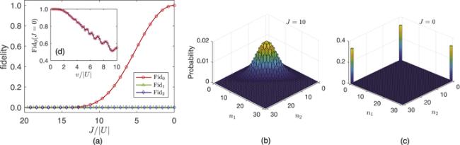
We adjust the decreasing rate v according to the adiabatic fidelity [59]. The ground state will evolve into the three-mode NOON state $| {{\mathfrak{T}}}_{0}\rangle $ at J = 0, if the decreasing rate is lower enough to meet the adiabatic condition. One can see the particle distribution changes from figures 3(b) to (c), equally distributed in ∣e1⟩, ∣e2⟩, and ∣e3⟩. Furthermore, the vanishing of the relative phases is verified numerically.
Figure 3. State preparation. (U = −0.5 and N = 30) (a) The fidelity versus J, where ${\mathrm{Fid}}_{a}=| \langle \psi (t)| {{\mathfrak{T}}}_{a}\rangle {| }^{2}$, for a = 0, 1, 2. J = J0 − vt with J0 = 10 and v = 0.2. ∣ψ(t)⟩ is the evolving state from the ground state at J = 10. Three-mode NOON state $| {{\mathfrak{T}}}_{0}\rangle $ is the target initial state. $\{| {{\mathfrak{T}}}_{0}\rangle ,| {{\mathfrak{T}}}_{1}\rangle ,| {{\mathfrak{T}}}_{2}\rangle \}$ are the orthogonal basis of the there-dimensional ground state manifolds ${{ \mathcal H }}_{N}$ at J = 0. (b)–(c) Distribution of quantum states in basis ∣n1, n2, n3⟩. (b) Ground state at J = 10. (c) ∣ψ(t)⟩ at J = 0, with v = 0.2. It is $| {{\mathfrak{T}}}_{0}\rangle $ approximately. (d) The inset shows the speed dependence of the state preparation via the final state fidelity Fid0 at J = 0 versus the speed v.
Intuitively speaking, this adiabatic process naturally presents a state in the three-dimensional ground state space ${{ \mathcal H }}_{N}$ at J = 0 in the adiabatic limit. The subtle point is that the state we prepared is $| {{\mathfrak{T}}}_{0}\rangle $ exactly. To show this result more rigorously, we introduce three basis states of the ground state space ${{ \mathcal H }}_{N}$, which reads $| {{\mathfrak{T}}}_{0}\rangle $, and $| {{\mathfrak{T}}}_{1(2)}\rangle =(| {e}_{1}\rangle +{{\rm{e}}}^{\pm {\rm{i}}2\pi /3}| {e}_{2}\rangle +{{\rm{e}}}^{\mp {\rm{i}}2\pi /3}| {e}_{3}\rangle )/\sqrt{3}$, respectively. Then we calculate the fidelity ${\mathrm{Fid}}_{a}=| \langle \psi (t)| {{\mathfrak{T}}}_{a}\rangle {| }^{2}$ for the whole adiabatic process, with a = 0, 1, 2, respectively. The result is plotted as figure 3(a). It shows Fid0 increases with decreasing J. Finally, we prepare the target state $| {{\mathfrak{T}}}_{0}\rangle $ at J = 0 almost certainly, as indicated by Fid0 ≈ 1. Meanwhile, fidelities of the other two states, Fid1 and Fid2, vanish not only for J = 0 but all J. It indicates that $| {{\mathfrak{T}}}_{1}\rangle $ and $| {{\mathfrak{T}}}_{2}\rangle $, hence, all of states in ${{ \mathcal H }}_{N}$ other than $| {{\mathfrak{T}}}_{0}\rangle $, are excluded in the whole adiabatic evolution. It is strong evidence that the state $| \psi {\rangle }_{{\mathfrak{i}}}$ we prepared is precisely the target state $| {{\mathfrak{T}}}_{0}\rangle $ in the adiabatic limit.
3.2. Parameterization and the QFI
In the last section, the three-mode NOON state $| {{\mathfrak{T}}}_{0}\rangle $ is prepared as the initial state of STWS. While keeping J = 0, we put the STWS in state $| {{\mathfrak{T}}}_{0}\rangle $ into an external field. Denote the shifted energy of mode ${\hat{a}}_{i}$ (ground state energy of the ith trap) in this field as ${{ \mathcal E }}_{i}$. Then the mode ${\hat{a}}_{i}$ will evolve as ${\hat{a}}_{i}{{\rm{e}}}^{{\rm{i}}{\phi }_{i}}$ with ${\phi }_{i}={{ \mathcal E }}_{i}t$, after time t. The state ${\left|\psi \right\rangle }_{{\mathfrak{i}}}$ is thus parameterized to the output state as
where θ = (θ1, θ2), with θi = φi − φ3, is the vector parameter to be estimated. We mention that the on-site interaction is negligible for it only contributes a global phase to ∣ψ(θ)⟩.
Substituting equation (12) into equation (7), we can calculate the four matrix elements of the QFIM on θ directly. The corresponding QFIM is
where ⟨Δ2θ⟩ ≡ ⟨Δ2θ1⟩ + ⟨Δ2θ2⟩ is the total variance of θ1 and θ2. Equation (14) indicates that the upper bound precision of estimating θ can approach the Heisenberg scaling.
3.3. Projective measurement
We have discussed the theoretical limit of the sensitivity via the QFIM. However, the accessible sensitivity highly depends on the measurement scheme. In this section, we focus on particle number measurement and study its precision with the CFIM.
In STWS, it is convenient to measure the particle number in each well on the final state. This measurement is depicted by a set of projection operators
with n = (n1, n2, n3). However, the phases will be eliminated if we directly perform this measurement on the parameterized state ∣ψ(θ)⟩. In this way, the parameter θ cannot be inferred. Hence, as the pretreatment of the measurement, we rotate the output state ∣ψ(θ)⟩ with
$\begin{eqnarray}{\hat{{ \mathcal U }}}_{R}(\tau )=\exp [-{\rm{i}}{\hat{H}}_{R}\tau /J],\end{eqnarray}$
with j = (i + 1) mod3 + 1. The tunneling strength J is fixed throughout the rotation. This Hamiltonian is valid when $J\gg \left|U\right|N$. It can be realized by both (1) increasing J via lowering the energy barrier between two traps and (2) tuning U ≈ 0 via the Feshbach resonance simultaneously. Based on equations (3), (12), and (16), we have the rotated final state as (see appendix A)
Applying the particle number measurement ${\hat{{\rm{\Pi }}}}_{{\boldsymbol{n}}}$ to the final state $| \psi {\rangle }_{{\mathfrak{f}}}$, we have the probability of acquiring results ∣n1, n2, n3⟩ as
The CFIM of probability Pn can be acquired directly via the definition equation (5). We denote it as Fc(θ, τ), for it depends on both the estimated vector θ and τ.
3.4. The optimal measurement precision
In this section, we will analyze the measurement precision with the gap Δ defined in equation (9). The optimal precision can be given by optimizing both the encoded parameters θ and rotation time τ.
Firstly, we discuss the dependence of Δ on θ with a given rotation time τ numerically. The results are shown in figure 4, where only one period is given. We observe that Δ highly depends on θ1 and θ2. For a given τ, the maximal precision can only be achieved in several points ‘•’. Luckily, with enough prior information provided, we can shift the estimand to the vicinity of these points to approach the maximal precision.
Figure 4. $\mathrm{ln}({\rm{\Delta }})$ versus (θ1, θ2) with a given τ. (a) τ = 0.2π. (b)τ = τO = 2π/9. The maximum precision (minimum of $\mathrm{ln}({\rm{\Delta }})$) for a given τ is marked as the black dots ‘•’. θG = (2π/3, 2π/3). Here, we set N = 30.
Secondly, by comparing figures 4(a) and (b), we find that the maximal precision over parameters θ highly depends on the rotation time τ. Specifically, we define
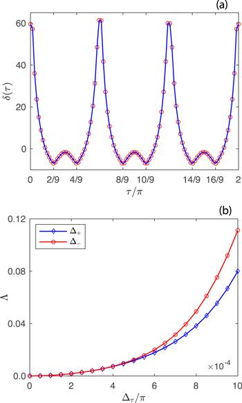
to study the effect of rotation time τ on the optimal precision over θ. As shown in figure 5(a), δ(τ) varies periodically with τ. There are three short periods with duration 2π/3 in a long period with duration 2π. More importantly, δ(τ) takes the minimum value at points
with $k\in {\mathbb{N}}$. We further show its validity numerically in figure 5(b), which indicates that τO = 2π/9 is one of the optimal rotation times.
Figure 5. (a) δ(τ) versus τ. (b) Λ versus Δτ. Λ = δ(τ) − δ(τO), ‘Δ±’ denote the line for τ = τO ± Δτ, with τO = 2π/9. Λ decreases to zero from above as Δτ approaches 0. Here, we set N = 30.
Now, one can acquire the optimal precision of our scheme by choosing the optimal phases (θ1, θ2) at an optimal time τ given in equation (21). It can be done numerically. An example with τ = τO = 2π/9 is given in figure 4(b), where the point ‘H’ is one of the optimal sets of phases.
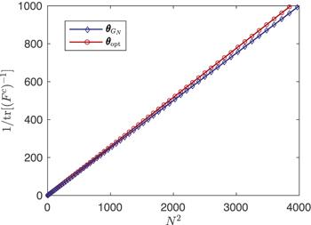
To evaluate the quality of the optimal precision, we study the scaling of CFIM with particle number N at τ = τO = 2π/9 both numerically and analytically. The numerical result is shown as the red line in figure 6. By searching the minimum of $\mathrm{tr}[{\left({{\boldsymbol{F}}}^{c}\right)}^{-1}]$ over the phase parameter θ at τO = 2π/9, we find the optimal precision satisfies the following linear relationship
It indicates a Heisenberg scaling precision. To show it more concretely, we further give a lower bound of the optimal precision analytically. The precision for the optimal phase point at τO is challenging to be given analytically. Hence, we calculate the precision for point ‘G’ instead, which is located near the optimal point ‘H’. The phase parameter ${{\boldsymbol{\theta }}}_{{G}_{N}}$ of the point ‘G’ is given by Nθ1 = Nθ2 = 2(N + 1)π/3, with N denoting the particle number. The CFIM of the state ‘G’ is (see appendix B)
The result is shown as the blue line in figure 6 in comparison with the optimal precision given by equation (22). It shows that the scaling of the two precisions is very close.
Figure 6. The precision ($1/\mathrm{tr}[{\left({{\boldsymbol{F}}}^{c}\right)}^{-1}]$) versus N2. Here, we set τ = τO = 2π/9. The red line denotes the numerical optimal precision. The blue line is analytical result at ${{\boldsymbol{\theta }}}_{{G}_{N}}$, which reads $\mathrm{tr}[{\left({{\boldsymbol{F}}}^{c}\right)}^{-1}]=4/{N}^{2}$.
We mention that equation (24) is valid for all particle numbers N. It indicates that, with the proposed measurement scheme, the optimal measurement precision of θ can always show a better Heisenberg scaling than equation (24). Furthermore, as indicated by figures 4(b) and 6, the precision is robust around the optimal parameters, e.g. ∣ψ(θG)⟩ with parameters θG still have relatively high precision with a Heisenberg scaling. It significantly reduces the demands for practical studies, which relieves the working parameters’ constrain from a point ‘H’ to, e.g. the white zoom in figure 4(b). With a relatively larger acceptance zoom of the parameter shifts, the demands for the prior information about the estimand θ are also highly reduced.
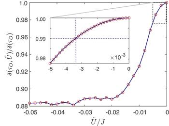
We have discussed the optimal precision under the projection measurement. However, the result is acquired under the approximation equation (17). If the on-site interaction between atoms cannot be tuned to zero precisely in the rotation operation, the total Hamiltonian reads
where $\tilde{U}$ denotes a small residual interaction induced by the imperfect control of the Feshbach resonance. To discuss the effect of residual interaction on the optimal precision, we define $\delta ({\tau }_{O},\tilde{U})$ as the generalization of δ(τO) (equation (20)) by substituting ${\hat{{ \mathcal U }}}_{R}({\tau }_{O})$ to the imperfect rotation
$\begin{eqnarray}{\hat{{ \mathcal U }^{\prime} }}_{R}({\tau }_{O})=\exp [-{\rm{i}}{\hat{H}}_{R}^{\prime} {\tau }_{O}/J].\end{eqnarray}$
$\delta ({\tau }_{O},\tilde{U})$ gives us the optimal precision over θ acquired under the imperfect rotation. We plot the ratio $\delta ({\tau }_{O},\tilde{U})$ as a function of $\tilde{U}$ in figure 7. Although $\delta ({\tau }_{O},\tilde{U})$ decreases with increasing $\tilde{U}$, the precision $\delta ({\tau }_{O},\tilde{U})$ is roughly on 99% of δ(τO) when $| N\tilde{U}/J| =0.1$. Even when $| N\tilde{U}/J| \approx 1$, i.e., the residual interactions and tunneling energy are on the same level, there still exists a platform around $\delta ({\tau }_{O},\tilde{U})=0.89\delta ({\tau }_{O})$. Thus, imperfect rotation with small residue interaction $\tilde{U}$ has acceptable influence on the optimal precision.
Figure 7. The precision $\delta ({\tau }_{O},\tilde{U})$ versus $\tilde{U}$, with τO = 2π/9. $\delta ({\tau }_{O},\tilde{U})$ is the optimal precision acquired via the imperfect rotation ${\hat{{ \mathcal U }}}_{R}^{{\prime} }({\tau }_{O})$. δ(τO) = δ(τO, 0). Here, we take J = 10, N = 30.
4. Conclusion and discussion
In this work, we have proposed a scheme for two-parameter estimation via a Bose–Einstein condensate confined in a symmetric triple-well potential. The three-mode NOON state has been prepared adiabatically as the initial state. The two parameters to be estimated are the two-phase differences between the wells, which are encoded into the initial state via the external fields. We perform the particle number measurement in each well to read the parameterized state. Moreover, a rotation operation is adopted on the output state before the measurement. We optimize both the parameters and rotation time to maximize the estimation precision. As a result, we have approached the Heisenberg scaling precision on simultaneous estimating two parameters under the optimal measurement.
We mention that our scheme is discussed in the ideal scenario in this article. To study it more rigorously, one should build an open quantum system model and introduce noise analysis based on practical experiments. We will advance this research in further studies. We expect to realize the high precision estimation of the two-dimensional fields, such as the magnetic field and gravity field, via ongoing research in this triple-well system.
Acknowledgments
F Y thanks Peng Wang for the helpful discussion. H X thanks Prof. Chang-Pu Sun for providing the valuable opportunity of visiting GSCAEP. This work was supported by the National Natural Science Foundation of China (NSFC) (Grant Nos. 12 088 101, 11 725 417, and U1930403) and Science Challenge Project (Grant No. TZ2018005).
Appendix A. The derivation of the rotated final state
The output state will be rotated by the operation ${\hat{{ \mathcal U }}}_{R}=\exp [-{\rm{i}}{\hat{H}}_{R}t]$. The Hamiltonian ${\hat{H}}_{R}=-J{\sum }_{i,j=1,i\ne j}^{3}{\hat{a}}_{i}^{\dagger }{\hat{a}}_{j}$ can be diagonalized in the basis
The output state $\left|\psi ({\boldsymbol{\theta }})\right\rangle $ can be transformed into the eigenbasis vector of ${\hat{H}}_{R}$ via equation (A2). The transformation of $\left|\psi ({\boldsymbol{\theta }})\right\rangle $ is thus given as below,
with θ3 = 0, n1 + n2 + n3 = N. It is equivalent to equation (18).
Appendix B. Scaling of the CFIM entries
In this section, we will show that: for a final state $| \psi {\rangle }_{{\mathfrak{f}}}$ with τ = 2π/9, there exist parameters ${{\boldsymbol{\theta }}}_{{G}_{N}}$ with Nθ1 = Nθ2 =(N + 1)2π/3, such that the QFI entries
We begin with the cases where the total particle number N = 3k, $k\in {{\mathbb{N}}}^{+}$. Set Nθ1 = Nθ2 = 2π/3, we have the probability of acquiring the result ∣n1, n2, n3⟩ as
The value of fμν(n) only depend on n $\mathrm{mod}$ 3. We list them in table B1. We mention that the coefficient of fμν(n) in equation (B5) is invariant under the arbitrary permutation of {n1, n2, n3}. Hence, fμν(n) can be further divided into three types with $\{{n}_{1},{n}_{2},{n}_{3}\}\mathrm{mod}3=\{0,0,0\}$, {1, 1, 1}, and {0, 1, 2}, respectively. And ${F}_{\mu \nu }^{c}$ is invariant under the substitution
Because, for a set of given {n1, n2, n3}, this substitution keeps the average of fμν(n) over the permutations of this set invariant. Furthermore, we have the summation:
We have thus shown the validity of equation (B1) for particle number N = 3k with $k\in {{\mathbb{N}}}^{+}$. Its validity for N = 3k + 1 and N = 3k + 2 can be verified with the same methods.
Table B1. Classification of fμν(n) with ${\boldsymbol{n}}\mathrm{mod}3$.


