


1. Introduction
Among the various higher-order derivative gravitational models described in the literature, Lovelock gravity [3] is quite special, as it is free of ghosts [4–10]. In fact, many of the higher-order derivative metric theories which have been presented exhibit Ostrogradsky instability (see [11, 12] for a good review). In this sense, the actions that contain higher-order curvature terms introduce equations of motion with fourth- or higher-order metric derivatives in which linear perturbations reveal that the graviton should be a ghost. Fortunately, the Lovelock model is free of ghost terms, and so has field equations involving no more than second-order derivatives of the metric. The action functional of Lovelock gravity is given by combinations of various terms, as follows. The first term is the cosmological constant Λ, the second term is the Ricci scalar $R={R}_{\mu }^{\mu },$ and the third and fourth terms are the second-order Gauss–Bonnet (GB) [13] and third-order Lovelock terms (see equation (22) in [14]), respectively. Without the latter term, the Lovelock gravity reduces to the simplest form called the Einstein–Gauss–Bonnet (EGB) theory, in which the Einstein–Hilbert action is supplemented with a quadratic curvature GB term as the source of the self-interaction of gravity. The importance of this form of the gravity model is more apparent when we observe that it is generated from the effective Lagrangian of low-energy string theory [15–19]. In fact, for more than four dimensions of curved space-time, the GB coupling parameter, which is calculated by the dimensional regularization method, has some regular values, but this is not the case for four dimensions. To resolve this problem, the author Glaven and his collaborator presented the proposal contained in [1], but we now know that their initial proposal does not lead to a very well-defined gravity theory, because regularization is guaranteed for just some metric theories and not for all of them. In this respect, the reader is referred to [20, 21], whose authors explained several inconsistencies in the original paper given by Glavan and Lin [1]. In particular, besides pointing out possible problems in defining the limit or finding an action for the theory, their work also adds new results to the discussion concerning the indefiniteness of second-order perturbations, even at a Minkowskian background, and the geodesic incompleteness of the spherically symmetric black hole geometry presented by Glavan and Lin (see also [22]).Thus, other proposals are needed that can cover all metric theories. In response to this problem, a well-defined and consistent theory was recently presented [2] that broke the diffeomorphism property of curved space-time. As opposed to the former work ([1]), the latter model is in concordance with the Lovelock theorem and therefore seems more to be physical and applicable. For instance, the Friedmann–Lemaître–Robertson–Walker cosmology of the latter model was studied in [23], which showed the success of this model compared to that of [1]. In fact, many papers about 4D EGB gravity and its applications in four or more dimensions of space-time have been published in the literature; one can see collections of these works mentioned in the introduction to reference [24]. Here, we point just to some of the newest works. For instance, the reader could view [25], whose authors obtained an exact static, spherically symmetric black hole solution in the presence of third-order Lovelock gravity, using a string cloud background in seven dimensions whose second-order and third-order Lovelock coefficients were related via ${\alpha }_{2}^{2}=3{\alpha }_{3}$. Furthermore, they examined the thermodynamic properties of this black hole to obtain exact expressions for mass, temperature, heat capacity, and entropy, and also performed a thermodynamic stability analysis. In their work, we see that a string cloud background has a profound influence on the horizon structure, thermodynamic properties, and stability of black holes. Interestingly, the entropy of the black hole is unaffected by the string cloud background. However, the critical solution for thermodynamic stability is affected by the string cloud background. Similar work was investigated by Toledo and his collaborator [26] in the presence of quintessence, but for different space-time dimensions. They showed graphs corresponding to the mass and Hawking temperature for different dimensions of space-time, such that D = 4, 5, 6, 7. By including Hawking radiation, it can be shown that the radiation spectrum is related to the change of entropy that codifies the presence of the cloud of strings as well as the presence of the quintessence. In their work, the importance of the number of space-time dimensions is shown by the thermal stabilization of the black holes affected by strings and surrounded with quintessence. By studying the relation between the Hawking temperature and entropy, they discussed the radiation rate and showed that this quantity depends on the change of entropy, which is given in terms of the event horizon and is strongly influenced by the presence of the cloud of strings as well as the presence of the quintessence. Therefore, the Hawking radiation spectrum depends strongly on the presence of the cloud of strings and on the quintessence. From this, one can infer that the presence of string clouds causes a black hole to be thermodynamically stable. Regarding the importance of the role of string theory in the study of black hole dynamics, we know that Juan Maldacena (see [27] for a good review), explained for the first time the development of a string theory interpretation of black holes in which quantum mechanics and general relativity, theories previously considered incompatible, are united. The work performed by Maldacena and others has given a precise description of a black hole, which is described holographically in terms of a theory living on the horizon. According to this theory, black holes behave like ordinary quantum mechanical objects—information about them is not lost, as previously thought, but retained on their horizons, leading physicists to look at black holes as laboratories for describing the quantum mechanics of space-time and for modeling strongly interacting quantum systems. Furthermore, the authors of [28] used model [1] to obtain an EGB spherically symmetric static charged black hole in the presence of Maxwell’s EM fields and a cloud of strings. They confirmed that as a result of correcting the black hole using the background cloud of string, the thermodynamic quantities were also corrected, except for the entropy, which remained unaffected by the cloud of string background. The Bekenstein–Hawking area law turns out to be corrected by a logarithmic area term. The heat capacity diverges to infinity at a critical radius where, incidentally, the temperature reaches a maximum, and the Hawking–Page transitions happen, even in absence of the cosmological term, by allowing the black hole to become thermodynamically stable. The smaller black holes with negative free energy are globally preferred. Their solution can also be identified as a 4D monopole-charged EGB black hole. In particular, their solution asymptotically reaches spherically symmetric black hole solutions of general relativity in the limit α → 0 and the absence of string tension.
In this work, we use the consistent EGB gravity model [2] in a minisuperspace approach and obtain the metric of a spherically symmetric static chargeless black hole in the presence of a cosmological parameter and Nambu–Goto string tension. The metric field equations are solved numerically, in which we use the Runge–Kutta methods to produce numeric values of the fields with best-fit functions. We then investigate the thermodynamic behavior of the obtained solution. To do so, we calculate the equation of state generated by the Hawking temperature of the black hole solution. In fact, in extended phase space, the cosmological constant plays an important role, namely, it represents the thermodynamic pressure of vacuum dS/AdS background space. In our obtained metric solutions we will see that the GB coupling constant plays a critical role in determining the scale of the black hole and the positions of the critical points in phase space where the black hole can participate in the small-to-large black hole phase transition in the dS sector and the Hawking–Page phase transition in the AdS sector. In the former case, diagrams of the pressure vs specific volume at a constant temperature (see figure 3(f)) behave similarly to those for a van der Waals gas/fluid, but this is not so for the latter case (see figure 4(f) in comparison to figure 3(f)). In fact, in the AdS sector, an unstable black hole finally reaches the AdS vacuum space.

Figure 1. P-T diagrams for ρ = 0 with the AdS background. The diagrams for the dS sector are similar to these curves, except where the pressures should be inverted according to $\bar{P}\to -\bar{P}$. |
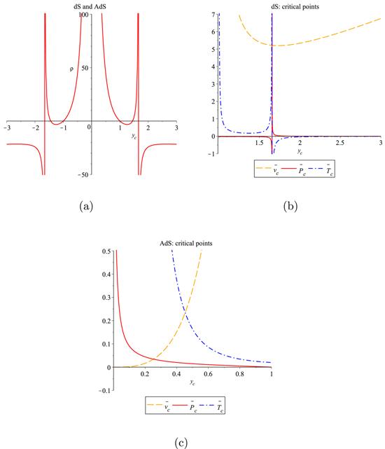
Figure 2. Numeric values of the critical points. |
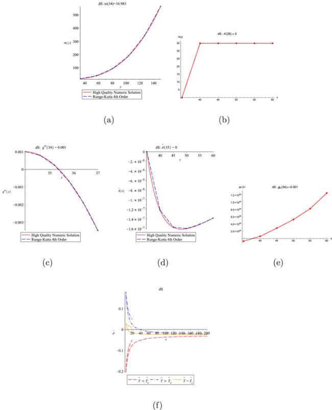
Figure 3. Diagrams of the numerical solutions of the fields for dS background space. The initial values used to produce the numerical solutions are shown at top of each diagram. |

Figure 4. Numerical solutions given by diagrams of the AdS sector. The initial values used to produce the numerical solutions are shown at the top of each diagram. |
The structure of this article is as follows: in section 2 , we recall the consistent 4D EGB gravity given by [2] and use a Nambu–Goto string fluid as the matter source of the system under consideration. In section 3 , we generate metric field equations for the spherically symmetric 4D black hole line element. In section 4 , we solve the metric field equations without string tension, i.e. such that the cosmological constant alone is the source. In this case, the field equations take on simpler forms and so we obtain an analytic form for the metric fields. In order to numerically solve the field equations in the presence of string tension, we provide some physical initial conditions in section 5 . In section 6 , we perform a numerical analysis of the solutions. The last section is devoted to the concluding remarks and the outlook.
2. 4D dS/AdS GB gravity with string fluid
According to [2], we know that a consistent EGB gravity theory in the D → 4 limit is given by the first part of the following action functional:2.1 ) is the absolute value of the determinant of the spatial metric γij. This ADM decomposition is performed on the background metric to remove divergent boundary terms of the higher-order metric derivative from the GB term of the action functional (2.1 ) in general 4D form [2]. The first term in the theory defined by (2.1 ) has the time reparametrization symmetry $t\to t=t({t}^{{\prime} }).$ We set the Lagrangian density of matter ${{ \mathcal L }}_{\mathrm{matter}}$ to be the Nambu–Goto action [29] (see also page 100 in [30]), which explains the dynamics of relativistic strings as follows:
$\begin{eqnarray}I=\displaystyle \frac{1}{16\pi G}\int {\rm{d}}t{{\rm{d}}}^{3}{xN}\sqrt{\gamma }({{ \mathcal L }}_{\mathrm{EGB}}^{4{\rm{D}}}+{{ \mathcal L }}_{\mathrm{matter}}),\end{eqnarray}$
in which the EGB geometrical Lagrangian density is $\begin{eqnarray}{{ \mathcal L }}_{\mathrm{EGB}}^{4D}=2R-2{\rm{\Lambda }}-{ \mathcal M }\end{eqnarray}$
$\begin{eqnarray*}\begin{array}{l}+\frac{\tilde{\alpha }}{2}[8{R}^{2}-4R{ \mathcal M }-{{ \mathcal M }}^{2}\\ -\frac{8}{3}(8{R}_{{ij}}{R}^{{ij}}-4{R}_{{ij}}{{ \mathcal M }}^{{ij}}-{{ \mathcal M }}_{{ij}}{{ \mathcal M }}^{{ij}})],\end{array}\end{eqnarray*}$
and the second part is the Lagrangian density of matter. The parameter G is Newton’s gravitational coupling constant, $R={R}_{i}^{i}({\gamma }_{{ij}})$ and Rij(γij) are the Ricci scalar and the Ricci tensor for the spatial metric γij, respectively, and $\begin{eqnarray}\begin{array}{l}{{ \mathcal M }}_{{ij}}={R}_{{ij}}+{{ \mathcal K }}_{k}^{k}{{ \mathcal K }}_{{ij}}-{{ \mathcal K }}_{{ik}}{{ \mathcal K }}_{j}^{k},\\ { \mathcal M }={{ \mathcal M }}_{i}^{i}\end{array}\end{eqnarray}$
with $\begin{eqnarray}\begin{array}{l}{{ \mathcal K }}_{{ij}}=\displaystyle \frac{1}{2N}({\dot{\gamma }}_{{ij}}-2{D}_{i}{N}_{j}-2{D}_{j}{N}_{i}-{\gamma }_{{ij}}{D}_{k}{D}^{k}{\lambda }_{\mathrm{GF}}).\end{array}\end{eqnarray}$
Here, a dot denotes the time derivative t, and all the effects of the constraint stemming from gauge fixing (GF) are now encoded in a Lagrange multiplier λGF; Di is the spatial covariant derivative, and the rescaled regular GB coupling constant $\tilde{\alpha }$ is defined versus the irregular GB coupling constant αGB in the limits of D → 4 dimensions such that $\tilde{\alpha }=(D-4){\alpha }_{{GB}}.$ The above EGB gravity action satisfies the following gauge condition for all spherically symmetric and cosmological backgrounds (see [2] and [23]): $\begin{eqnarray}\sqrt{\gamma }{D}_{k}{D}^{k}({\pi }^{{ij}}{\gamma }_{{ij}}/\sqrt{\gamma })\approx 0.\end{eqnarray}$
In fact, the above EGB action is rewritten versus the 1 + 3 Arnowitt-Deser-Misner (ADM) decomposition of the 4D background metric, for which $\begin{eqnarray}\begin{array}{l}{{\rm{d}}{s}}^{2}={g}_{\mu \nu }{{\rm{d}}{x}}^{\mu }{{\rm{d}}{x}}^{\nu }=-{N}^{2}{{\rm{d}}{t}}^{2}+{\gamma }_{{ij}}({{\rm{d}}{x}}^{i}+{N}^{i}{\rm{d}}{t})({{\rm{d}}{x}}^{j}+{N}^{j}{\rm{d}}{t}),\end{array}\end{eqnarray}$
where N, Ni, and γij are the lapse function, the shift vector, and the spatial metric, respectively. The γ factor in the action ( $\begin{eqnarray}{I}_{\ \mathrm{NG}}=-{\int }_{{\rm{\Sigma }}}{{ \mathcal L }}_{\mathrm{NG}}{\rm{d}}{\sigma }^{0}{\rm{d}}{\sigma }^{1},\end{eqnarray}$
in which $\begin{eqnarray}{{ \mathcal L }}_{\mathrm{NG}}=\rho \sqrt{{\mathfrak{g}}}=\rho {\left(-\displaystyle \frac{1}{2}{{\rm{\Sigma }}}^{\mu \nu }{{\rm{\Sigma }}}_{\mu \nu }\right)}^{ \frac{1}{2}}\end{eqnarray}$
is the Lagrangian density, and the constant parameter ρ is the tension or proper density of the string. In addition, the bivector Σμν is related to the string worldsheet parameters (σ0, σ1) such that $\begin{eqnarray}{{\rm{\Sigma }}}^{\mu \nu }={\epsilon }^{{ab}}\frac{\partial {x}^{\mu }}{\partial {\sigma }^{a}}\frac{\partial {x}^{\nu }}{\partial {\sigma }^{b}},\end{eqnarray}$
for which εab is the two-dimensional Levi-Civita tensor density ε01 = − ε10 = 1, and ${\mathfrak{g}}$ is the absolute value of the determinant of the induced metric $\begin{eqnarray}{{\mathfrak{g}}}_{{ab}}={g}_{\mu \nu }\displaystyle \frac{\partial {x}^{\mu }}{\partial {\sigma }^{a}}\displaystyle \frac{\partial {x}^{\nu }}{\partial {\sigma }^{b}}.\end{eqnarray}$
The stress-energy tensor of this relativistic string is given by $\begin{eqnarray}{T}^{\mu \nu }={{\mathfrak{g}}}^{-\tfrac{1}{2}}\rho {{\rm{\Sigma }}}^{\mu \delta }{{\rm{\Sigma }}}_{\delta }^{\nu }=\displaystyle \frac{2\partial {{\mathfrak{L}}}_{{NG}}}{\partial {g}^{\mu \nu }}\end{eqnarray}$
and its covariant conservation reads ∇μ(ρΣμν) = 0. In order for Tμν to be invariant under a reparametrization of the string’s world sheets, ρ must be transformed as ${{\mathfrak{g}}}^{-1/2}$ (see [29] and references therein). We are now in a position to use the above model for a spherically symmetric static black hole space-time.3. 4D dS/AdS Gauss Bonnet black hole surrounded by string cloud
By comparing the line element (2.6 ) with the general anisotropic form of a spherically symmetric static 4D curved metric3.1 ) into (2.2 ), we obtain3.1 ), we should solve ∇μ(ρΣμν) = 0. However, this equation is equivalent to ${\partial }_{\mu }(\rho \sqrt{g}{{\rm{\Sigma }}}^{\mu \nu })=0$ because of the antisymmetric property of the bivector Σμν. The spherically symmetric property of space-time (3.1 ) causes only r to depend on the string Lagrangian density. Thus we can show that the equation ${\partial }_{\mu }(\rho \sqrt{g}{{\rm{\Sigma }}}^{\mu \nu })=0$ leads to the following solution for the metric equation (3.1 ):2.8 ), yields2.7 ) using a static gauge [30] in which the commoving time σ0 in the parameter space xμ(σ0, σ1) of the worldsheet is equal to the time t in target space as ${\sigma }^{0}=t={t}_{0}={constant}$, and we should assume that the static string is aligned in the radial direction r of the worldsheet xμ(σ0, σ1) such that2.10 ) read as follows:3.8 ) and (3.9 ) into (2.7 ), we integrate on the worldsheet Σ as3.1 ). This is done by replacing the 4D covariant differential volume element for the line element (3.1 ) given by3.7 ), allows us to infer that3.3 ), (3.2 ), and (3.13 ) into the total action functional (2.1 ) and by integrating angular parts on the 2-sphere 0 ≤ θ ≤ π, 0 ≤ φ ≤ 2π, we obtain3.4 ) and the action functional (3.14 ) leads to the following forms, respectively3.22 ) has the following boundary condition3.20 ) dimensionless, as follows.3.23 ) and equation (3.21 ) reduces to the following forms, respectively:3.26 ) as follows:3.27 ), we can infer that the negative branch y < 0 corresponds to $b=-\sqrt{\tilde{\alpha }}$, while the positive branch y > 0 corresponds to $b=+\sqrt{\tilde{\alpha }}$, because, in both cases, we have r > 0. By substituting the definition
$\begin{eqnarray}\begin{array}{l}{{\rm{d}}{s}}^{2}=-{{\rm{e}}}^{2A(r)}\left(1-\frac{2M(r)}{r}\right){{\rm{d}}{t}}^{2}\\ +\frac{{{\rm{d}}{r}}^{2}}{1-\frac{2M(r)}{r}}+{r}^{2}{\rm{d}}{\theta }^{2}+{r}^{2}{\sin }^{2}\theta {\rm{d}}{\varphi }^{2},\end{array}\end{eqnarray}$
we obtain $\begin{eqnarray}N={{\rm{e}}}^{A(r)}\sqrt{1-\displaystyle \frac{2M(r)}{r}},\,\,\,{N}_{r,\theta ,\varphi }=0,\end{eqnarray}$
$\begin{eqnarray*}\begin{array}{l}{\gamma }_{{rr}}=\displaystyle \frac{1}{1-\tfrac{2M(r)}{r}}\,\,\,{\gamma }_{\theta \theta }={r}^{2},\\ {\gamma }_{\varphi \varphi }={r}^{2}{\sin }^{2}\theta ,\,\,\,{\lambda }_{\mathrm{GF}}={\lambda }_{\mathrm{GF}}(r).\end{array}\end{eqnarray*}$
By substituting ( $\begin{eqnarray}\begin{array}{l}{{ \mathcal L }}_{\mathrm{EGB}}^{4{\rm{D}}}=R({\gamma }_{{ij}})-2{\rm{\Lambda }}+12{q}^{2}\\ +\displaystyle \frac{\tilde{\alpha }}{2}\left[3{R}^{2}(\gamma )+\displaystyle \frac{88}{3}{q}^{2}R(\gamma )-272{q}^{4}-8{R}_{{ij}}(\gamma ){R}^{{ij}}(\gamma )\right]\end{array}\end{eqnarray}$
in which $\begin{eqnarray}q(r)=\displaystyle \frac{{{\rm{e}}}^{-A(r)}}{{r}^{2}}{\left[{r}^{2}{\lambda }_{{GF}}^{{\prime} }(r)\right]}^{{\prime} },\,\,\,{{ \mathcal K }}_{{ij}}=-q{\gamma }_{{ij}}\end{eqnarray}$
$\begin{eqnarray}R(\gamma )=-\displaystyle \frac{4{M}^{{\prime} }}{{r}^{2}},\,\,\,{R}_{{ij}}(\gamma ){R}^{{ij}}(\gamma )=\displaystyle \frac{6}{{r}^{6}}{\left(M-{{rM}}^{{\prime} }\right)}^{2}\end{eqnarray}$
and ′ (prime) denotes the derivative with respect to r. To obtain the explicit form of the Lagrangian density of the NG string for the line element ( $\begin{eqnarray}{{\rm{\Sigma }}}^{{rt}}(r)=\displaystyle \frac{{{c}{\rm{e}}}^{-A(r)}}{\rho {r}^{2}},\,\,\,{{\rm{\Sigma }}}_{{rt}}(r)=-\displaystyle \frac{{{c}{\rm{e}}}^{A(r)}}{\rho {r}^{2}}\end{eqnarray}$
which, substituted into the Lagrangian density ( $\begin{eqnarray}{{ \mathcal L }}_{{NG}}=\displaystyle \frac{c}{{r}^{2}}\end{eqnarray}$
in which c is an integral constant that should be fixed by the physical characteristic of the string, namely, its tension ρ. To do so, we calculate the integral equation ( $\begin{eqnarray}\begin{array}{l}r=r({\sigma }^{0},{\sigma }^{1})=F({\sigma }^{1}),\qquad t={\sigma }^{0},\\ \theta ({\sigma }^{0},{\sigma }^{1})=\varphi ({\sigma }^{0},{\sigma }^{1})=0.\end{array}\end{eqnarray}$
Here, we choose an open string for which one edge of the worldsheet is the curve σ1 = 0 and the other edge is the curve σ1 = a, such that σ1 ∈ [0, a] for an open string with the arbitrary shape F(σ1). In any case, if the central object is a black hole, the string fluid would naturally be attracted/absorbed by it, and the system would be time-dependent. In order for the string fluid to be in equilibrium with the black hole, it must satisfy some specific conditions, such as, for example, the formation of a disk, and for the strings to move on marginally stable orbits outside the event horizon. Even if we assume that the background metric is spherically symmetric but not static and also that the string tension is time-dependent, there is no doubt about the stable time-independent metric solutions that we consider here, because the author of [28] proved that the spherically symmetric static conditions of a curved space-time cause it to be time independent of the NG string cloud stress tensor and it is a general solution of the Einstein metric equation. In other words, we have a ‘Birkhoff theorem’ for the cloud of strings and so the metric solution is the general solution for the symmetry under consideration. In this case, the non-vanishing components of the induced metric ( $\begin{eqnarray}\begin{array}{l}{{\mathfrak{g}}}_{11}=-{{\rm{e}}}^{2A(r)}\left(1-\displaystyle \frac{2M(r)}{r}\right),\\ {{\mathfrak{g}}}_{22}=\displaystyle \frac{1}{\left(1-\tfrac{2M(r)}{r}\right)}{\left(\displaystyle \frac{{\rm{d}}{F}({\sigma }^{1})}{{\rm{d}}{\sigma }^{1}}\right)}^{2},\end{array}\end{eqnarray}$
$\begin{eqnarray*}\sqrt{{\mathfrak{g}}}=\sqrt{| {\rm{\det }}({\mathfrak{g}})| }={{\rm{e}}}^{A}\displaystyle \frac{{dF}({\sigma }^{1})}{d{\sigma }^{1}}.\end{eqnarray*}$
By substituting ( $\begin{eqnarray}\begin{array}{l}{I}_{\mathrm{NG}}=-{\displaystyle \int }_{0}^{t}{\rm{d}}t{\displaystyle \int }_{0}^{a}\rho {{\rm{e}}}^{A}\left(\displaystyle \frac{{\rm{d}}{F}({\sigma }^{1})}{{\rm{d}}{\sigma }^{1}}\right){\rm{d}}{\sigma }^{1}\\ =-{\displaystyle \int }_{0}^{t}{\rm{d}}t{\displaystyle \int }_{0}^{r(a)}\rho {{\rm{e}}}^{A}{\rm{d}}r.\end{array}\end{eqnarray}$
We should now obtain a changed form of the above equation from the parameter space of the worldsheet for the target space-time ( $\begin{eqnarray}{\rm{d}}{v}^{[4]}=\sqrt{g}{\rm{d}}{x}^{4}=4\pi {r}^{2}{{\rm{e}}}^{A}{\rm{d}}r{\rm{d}}t\end{eqnarray}$
with a two-dimensional parameter differential surface dσ0dσ1 ≡ eAdtdr in the above equation. As a result, we obtain $\begin{eqnarray}{I}_{\mathrm{NG}}=-\int \left(\displaystyle \frac{\rho }{4\pi {r}^{2}}\right){\rm{d}}{v}^{[4]}\end{eqnarray}$
which, when compared with ( $\begin{eqnarray}{{ \mathcal L }}_{\mathrm{NG}}=\displaystyle \frac{\rho }{4\pi {r}^{2}},\,\,\,c=\displaystyle \frac{\rho }{4\pi .}\end{eqnarray}$
By substituting ( $\begin{eqnarray}\begin{array}{l}I=\displaystyle \frac{1}{4G}\displaystyle \int {\rm{d}}t\displaystyle \int {\rm{d}}{{rr}}^{2}{{\rm{e}}}^{A(r)}\\ \left\{-\displaystyle \frac{4{M}^{{\prime} }}{{r}^{2}}-2{\rm{\Lambda }}+12{q}^{2}-\displaystyle \frac{\rho }{4\pi {r}^{2}}\right.\end{array}\end{eqnarray}$
$\begin{eqnarray*}\begin{array}{l}-\tilde{\alpha }\left[\displaystyle \frac{176{M}^{{\prime} }{q}^{2}}{3{r}^{2}}+136{q}^{4}\right.\\ \left.\left.+\displaystyle \frac{24{M}^{2}}{{r}^{6}}-\displaystyle \frac{48{{MM}}^{{\prime} }}{{r}^{5}}\right]\right\}.\end{array}\end{eqnarray*}$
The Euler–Lagrange equation for q reads $\begin{eqnarray}q\left[12-\tilde{\alpha }\left(\displaystyle \frac{176{M}^{{\prime} }}{3{r}^{2}}+136{q}^{2}\right)\right]=0\end{eqnarray}$
which has two different solutions: $\begin{eqnarray}{q}_{1}=0,\,\,\,{q}_{2}=\displaystyle \frac{\pm 1}{\sqrt{136}}\sqrt{\displaystyle \frac{12}{\tilde{\alpha }}-\displaystyle \frac{176{M}^{{\prime} }}{3{r}^{2}}}.\end{eqnarray}$
Substituting q1,2 into equation ( $\begin{eqnarray}{\lambda }_{\mathrm{GF}}^{(1)}(r)\sim \displaystyle \frac{1}{r}\end{eqnarray}$
$\begin{eqnarray}{\lambda }_{\mathrm{GF}}^{(2)}(r)={\int }^{r}\displaystyle \frac{{\rm{d}}{r}^{{\prime} }}{{r}^{{\prime} 2}}{\int }^{{r}^{{\prime} }}{\left({r}^{{\prime\prime} }\right)}^{2}{q}_{2}({r}^{{\prime\prime} }){{\rm{e}}}^{A({r}^{{\prime\prime} })}{\rm{d}}{r}^{{\prime\prime} }\end{eqnarray}$
and $\begin{eqnarray}{I}_{1}={I}_{2}=\displaystyle \frac{1}{4G}\int {\rm{d}}t\int {\rm{d}}{{rr}}^{2}{{\rm{e}}}^{A(r)}\left\{-\displaystyle \frac{4{M}^{{\prime} }}{{r}^{2}}-2{\rm{\Lambda }}-\right.\end{eqnarray}$
$\begin{eqnarray*}\left.\displaystyle \frac{\rho }{4\pi {r}^{2}}+\tilde{\alpha }\left[-\displaystyle \frac{24{M}^{2}}{{r}^{6}}+\displaystyle \frac{48{{MM}}^{{\prime} }}{{r}^{5}}\right]\right\}.\end{eqnarray*}$
The Euler–Lagrange equations for the function A(r) and the mass distribution function M(r) reduce to the following relations, respectively. $\begin{eqnarray}\displaystyle \frac{4{M}^{{\prime} }}{{r}^{2}}=\displaystyle \frac{-\tfrac{\rho }{4\pi {r}^{2}}-2{\rm{\Lambda }}-\tfrac{24\tilde{\alpha }{M}^{2}(r)}{{r}^{6}}}{1-\tfrac{12\tilde{\alpha }M(r)}{{r}^{3}}}\end{eqnarray}$
and $\begin{eqnarray}{A}^{{\prime} }(r)=\displaystyle \frac{\tfrac{-24\tilde{\alpha }M}{{r}^{4}}}{1-\tfrac{12\tilde{\alpha }M(r)}{{r}^{3}}}.\end{eqnarray}$
We are now in a position to solve the above nonlinear differential equations. This is done via a numerical approach in this work. To do so, we need the physical boundary conditions, as follows. We know that the mass distribution function M(r) is related to the matter density function ρM by $\begin{eqnarray}M(r)={\int }_{0}^{r}4\pi {r}^{2}{\rho }_{{\rm{M}}}(r){\rm{d}}r,\end{eqnarray}$
for which we can write $\begin{eqnarray}{\rho }_{{\rm{M}}}=\displaystyle \frac{{M}^{{\prime} }}{4\pi {r}^{2}}.\end{eqnarray}$
On the other side, i.e. the outside region of the gravitational compact object (the vacuum zone) with radius R, we have $\begin{eqnarray}{\rho }_{{\rm{M}}}(r)=0,\,\,\,r\gt R,\end{eqnarray}$
while for any arbitrary form of the density function ρM(r), the mass integral equation ( $\begin{eqnarray}M(0)=0.\end{eqnarray}$
To study the dynamics of the compact object, it is useful to make equation ( $\begin{eqnarray}\dot{m}(y)=\displaystyle \frac{-\tfrac{\rho }{16\pi }-\tfrac{{\rm{\Lambda }}{b}^{2}}{2}{y}^{2}-\tfrac{{m}^{2}}{{y}^{4}}}{1-\tfrac{2m}{{y}^{3}}}\end{eqnarray}$
where the dot $\dot{}$ represents differentiation with respect to y and we define $\begin{eqnarray}m(y)=\displaystyle \frac{M(r)}{b},\,\,\,y=\displaystyle \frac{r}{b},\,\,\,b=\pm \sqrt{6\tilde{\alpha }}.\end{eqnarray}$
In this case, the dimensionless form of the mass density ( $\begin{eqnarray}\begin{array}{l}{D}_{{\rm{M}}}=8\pi {b}^{2}{\rho }_{{\rm{M}}}(y)=\displaystyle \frac{\dot{m}}{{y}^{2}}=\displaystyle \frac{-\tfrac{\rho }{16\pi {y}^{2}}-\tfrac{{\rm{\Lambda }}{b}^{2}}{2}-\tfrac{{m}^{2}}{{y}^{6}}}{1-\tfrac{2m}{{y}^{3}}}\end{array}\end{eqnarray}$
and $\begin{eqnarray}\dot{A}(y)=\displaystyle \frac{-\tfrac{4m}{{y}^{4}}}{1-\tfrac{2m}{{y}^{3}}}.\end{eqnarray}$
We end this section of the paper by giving the radius of the gravitational compact object and the corresponding horizons. The position of the radius is obtained by solving $\dot{m}=0$, such that $\begin{eqnarray}{y}_{R}=\displaystyle \frac{\pm 1}{4}\sqrt{\displaystyle \frac{-\rho \pm \sqrt{{\rho }^{2}-128{\pi }^{2}{\rm{\Lambda }}{b}^{2}/{s}^{2}}}{2\pi s{\rm{\Lambda }}{b}^{2}}}\end{eqnarray}$
where we use yR = 2sm(yR) with s ≥ 1, and its horizons are obtained by substituting the horizon hypersurface y = 2m(y) with $\dot{m}=\tfrac{1}{2}$ into equation ( $\begin{eqnarray}{{y}_{{\rm{H}}}}_{\pm }=\displaystyle \frac{\pm 1}{\sqrt{1+\tfrac{\rho }{8\pi }\mp \sqrt{{\left(1+\tfrac{\rho }{8\pi }\right)}^{2}+2{b}^{2}{\rm{\Lambda }}}}}.\end{eqnarray}$
By looking at the definition $b=\pm \sqrt{6\tilde{\alpha }}$ given by ( $\begin{eqnarray}{\ell }=\displaystyle \frac{{y}_{{\rm{H}}}}{{y}_{{\rm{R}}}}\end{eqnarray}$
into the above relations, for particular limiting choice s = 1, we obtain $\begin{eqnarray}\begin{array}{l}\frac{\rho }{4\pi }=\frac{{\ell }^{4}-2{y}_{{\rm{H}}}^{2}+1}{{y}_{{\rm{H}}}^{2}(1-{\ell }^{2})},\\ 2{b}^{2}{\rm{\Lambda }}=\frac{{\ell }^{2}[{\ell }^{2}-2{y}_{{\rm{H}}}^{2}+1]}{{y}_{{\rm{H}}}^{4}({\ell }^{2}-1)},\end{array}\end{eqnarray}$
where we must choose 0 < ℓ < 1 for a star solution and ℓ > 1 for a black hole solution. By applying the positivity condition of the string tension ρ ≥ 0 to the above relations, we obtain $\begin{eqnarray}{\rm{Star}}:\,\,\,\,\,{\ell }\lt 1,\,\,\,2{y}_{{\rm{H}}}^{2}\lt 1+\displaystyle \frac{1}{{{\ell }}^{4}}\end{eqnarray}$
$\begin{eqnarray*}{\rm{Black}}\,{\rm{hole}}:\,\,\,{\ell }\gt 1,\,\,\,2{y}_{{\rm{H}}}^{2}\gt 1+\displaystyle \frac{1}{{{\ell }}^{4}}.\end{eqnarray*}$
It is easy to see that for the dS sector Λ > 0 the positive signs in the above horizon positions are valid, but in the case of AdS with Λ < 0, both the positive and negative signs may be valid and reduce to two different real values. In the latter case, we will call the smaller horizon the black hole horizon and the larger one the modified cosmological horizon. Without the cosmological parameter Λ = 0, the above equation gives us a curved space-time with one horizon such that $\begin{eqnarray}{y}_{{\rm{H}}}=\sqrt{\displaystyle \frac{4\pi }{8\pi +\rho }},\,\,\,{\rm{\Lambda }}=0,\,\,\,{y}_{{\rm{R}}}=\displaystyle \frac{{y}_{{\rm{H}}}}{\sqrt{2{y}_{{\rm{H}}}^{2}-1}}.\end{eqnarray}$
We now proceed to solve the above dynamical equations for different situations, as follows.4. Solutions with ρ = 0, Λ(> , < , =)0
The equation (3.26 ) has an analytic exact solution in the absence of string tension:3.29 ) reads3.33 ) reads4.1 ) shows that we must choose4.1 ) reads4.6 ) and (4.7 ) are plotted in figures 1(b), (c), and (d). These diagrams show a dS/AdS phase transition with a coexistence state (the swallow tail in figure 1(c)) between them at the crossing point in the P-T diagrams.
$\begin{eqnarray}m(y)=\zeta {y}^{3},\,\,\,\zeta =\displaystyle \frac{3\pm \sqrt{9+10{b}^{2}{\rm{\Lambda }}}}{10},\,\,\,\rho =0\end{eqnarray}$
for which equation ( $\begin{eqnarray}A(y)=\left(\displaystyle \frac{4\zeta }{2\zeta -1}\right)\mathrm{ln}(y)\end{eqnarray}$
with the corresponding metric components $\begin{eqnarray}{g}^{{rr}}(y)=1-2\zeta {y}^{2},\,\,\,{g}_{\mathrm{tt}}(y)=-{y}^{\tfrac{8\zeta }{2\zeta -1}}(1-2\zeta {y}^{2}).\end{eqnarray}$
In this case, for 2ζ > 1, we have one apparent horizon at position ${y}_{\mathrm{AH}}=\tfrac{1}{\sqrt{2\zeta }}$ and two event horizons at positions yEH = 0 and yEH = yAH. For 0 < 2ζ < 1, the position of the event horizon yEH moves to infinity, yEH → ∞, and ( $\begin{eqnarray}{\ell }={\left(\displaystyle \frac{1}{\zeta }-1\right)}^{ \frac{1}{4}}.\end{eqnarray}$
This shows that for $\zeta \gt \tfrac{1}{2}$, we have a black hole in which ℓ < 1, and so yR < yH, while for $0\lt \zeta \lt \tfrac{1}{2}$, we have yR > yH and so the above metric is not a black hole but perhaps a regular star. The definition of ζ in relation ( $\begin{eqnarray}{\rm{\Lambda }}\geqslant \displaystyle \frac{-3}{20\tilde{\alpha }}.\end{eqnarray}$
This can be understood as follows: the unknown cosmological constant in the general theory of relativity originates, in fact, from the GB coupling parameter and is therefore comprehensible. According to the relationship $\tilde{\alpha }=(D-4){\alpha }_{\mathrm{GB}}$ and the positivity condition of the GB coupling constant αGB > 0, we infer that the above relationship corresponds to a AdS (dS) space when $\tilde{\alpha }\gt 0(\lt 0)$ and so D > 4 ( < 4). This means that when we regularize the GB action functional, it should be done by limiting from higher space-time dimensions to 4D for AdS space and vice versa for dS space. For the above analytic metric solution, it is easy to show that the Hawking temperature $\bar{T}={bT}=-\tfrac{1}{2\pi }{\tfrac{{\rm{d}}{g}_{\mathrm{tt}}(y)}{{\rm{d}}y}}_{| {y}_{{\rm{H}}}}$ reads $\begin{eqnarray}\bar{T}=2{\left(2\zeta \right)}^{\tfrac{1}{2}\left(\tfrac{1+6\zeta }{1-2\zeta }\right)}.\end{eqnarray}$
We know that at the extended phase space, the pressure of AdS space is defined by $P=-\tfrac{{\rm{\Lambda }}}{8\pi }$ for negative values of the cosmological constant Λ < 0 and $P=\tfrac{{\rm{\Lambda }}}{8\pi }$ for the dS sector with Λ > 0. Considering these definitions, the parameter ζ given by ( $\begin{eqnarray}\bar{P}={b}^{2}P=\displaystyle \frac{\pm [{\left(10\zeta -3\right)}^{2}-9]}{80\pi }\end{eqnarray}$
where + ( − ) corresponds to the dS(AdS) sector. For pressureless space Λ = 0, we have ζ = {0, 0.6} for which the corresponding temperatures are T(0) = 0 and T(0.6) = 0.1422. The metric field solution is a flat Minkowski space-time for ζ = 0 but not for ζ = 0.6. Figure 1(a) shows the event and apparent horizons of space-time in the latter case, in which their positions are points at which the horizontal axes are crossed. The event horizon is obtained by solving gtt(y) = 0, and the apparent horizon is obtained with grr(y) = 0 for spherically symmetric state space-times. Pressure-temperature phase diagrams for equations (5. Initial conditions with ρ > 0, Λ( > , < , = )0
For the case ρ ≠ 0, equation (3.26 ) has no analytic solution and it has to be solved via numerical methods. To do so, we apply the Runge–Kutta methods, for which we should assume some physical initial conditions for m(y), ρ, Λ, and the y domain. By looking at equation (3.25 ), one can infer that a suitable initial condition for the mass parameter is3.20 ), (3.21 ), and definition (3.27 ) into the Hawking temperature (5.2 ) to obtain the 4D GB black hole equation of state, such that3.26 ) and (3.29 ). We will address this in the next section. By substituting the above critical points into equations (3.33 ), we obtain two classes of solution, one of which relates to stars, ℓ < 1, and the other of which relates to black hole, ℓ > 1, as follows:3.33 ), because the solutions in the regions with y < 0 are positioned in the analytic continuation of y in the complex algebraic analysis. We also substitute ${P}_{{\rm{c}}}=\tfrac{{\rm{\Lambda }}}{8\pi }$ and ${P}_{{\rm{c}}}=-\tfrac{{\rm{\Lambda }}}{8\pi }$ into the above critical points to obtain5.12 ) and the star choice in (5.13 ) are not physical, because, for these cases, the thermodynamic specific volume takes on a negative sign. Thus, in the next section, we proceed to solve (3.26 ) and (3.29 ) for just the star choice in the AdS and just the black hole choice in the dS sector.
$\begin{eqnarray}m(0)=0,\end{eqnarray}$
while we are still free to choose various values for Λ, ρ, and the regimes of the variable y. To determine the suitable regimes for these parameters, we obtain the equation for the state of the system by calculating the corresponding Hawking temperature, as follows. We know that the Hawking temperature of a black hole space-time is determined by the value of surface gravity on its exterior horizon such that $\begin{eqnarray}\begin{array}{l}T=\displaystyle \frac{-1}{4\pi }{\displaystyle \frac{{\rm{d}}{g}_{\mathrm{tt}}(r)}{{\rm{d}}r}}_{| r=2M(r)}=\displaystyle \frac{{{\rm{e}}}^{2A(r)}}{2\pi }\\ {\left[{A}^{{\prime} }(r)\left(1-\displaystyle \frac{2M(r)}{r}\right)+\displaystyle \frac{M(r)}{{r}^{2}}-\displaystyle \frac{{M}^{{\prime} }(r)}{r}\right]}_{{| }_{{\rm{r}}=2{\rm{M}}({r})}}.\end{array}\end{eqnarray}$
For an AdS (dS) background with a pressure of $P\,=\tfrac{-{\rm{\Lambda }}}{8\pi }\gt 0\,(P=\tfrac{{\rm{\Lambda }}}{8\pi }\gt 0)$, we substitute ( $\begin{eqnarray}\begin{array}{l}{\rm{AdS}}:\,\,\,\bar{T}=\bar{P}\bar{v}-\bar{v}f(\bar{v}),\\ \bar{v}=\displaystyle \frac{v}{b}=\displaystyle \frac{2{y}^{3}{{\rm{e}}}^{2A(y)}}{1-{y}^{2}},\,\,\,0\leqslant y\leqslant 1\end{array}\end{eqnarray}$
and $\begin{eqnarray}\begin{array}{l}{\rm{dS}}:\,\,\,\bar{T}=\bar{P}\bar{v}+\bar{v}f(\bar{v}),\\ \bar{v}=\displaystyle \frac{v}{b}=\displaystyle \frac{2{y}^{3}{e}^{2A(y)}}{{y}^{2}-1},\,\,\,y\geqslant 1\end{array}\end{eqnarray}$
where $\bar{v}$ is a dimensionless specific volume and $\begin{eqnarray}f[\bar{v}(y)]=\displaystyle \frac{1}{4\pi {y}^{2}}\left[\displaystyle \frac{1}{2}+\displaystyle \frac{\rho }{16\pi }-\displaystyle \frac{1}{4{y}^{2}}\right].\end{eqnarray}$
By looking at the above equation of state, one can infer that at large scales (y → ∞), the function $f(\bar{v})$ vanishes and so the above equation of state reaches the well-known ideal gas equation of state. We are now in a position to obtain the critical point in T-v extended phase space. This is done by calculating the equation of the critical points $\tfrac{\partial T}{\partial v}{| }_{P}=0$ and $\tfrac{{\partial }^{2}T}{\partial {v}^{2}}{| }_{P}=0$, which can be reduced to the following conditions by considering the chain rule in the derivatives: $\begin{eqnarray}\frac{\partial \bar{T}}{\partial y}{| }_{P}=0,\,\,\,\frac{{\partial }^{2}\bar{T}}{\partial {y}^{2}}{| }_{P}=0.\end{eqnarray}$
The above equations give us a parametric critical point such that for AdS we have $\begin{eqnarray}\begin{array}{l}{\rm{AdS}}:\,\,\,{\bar{P}}_{{\rm{c}}}({y}_{{\rm{c}}})\\ =\displaystyle \frac{-3({y}_{{\rm{c}}}^{4}+2{y}_{{\rm{c}}}^{2}+5)}{16\pi {y}_{{\rm{c}}}^{4}({y}_{{\rm{c}}}^{4}+10{y}_{{\rm{c}}}^{2}-35)},\end{array}\end{eqnarray}$
$\begin{eqnarray*}\begin{array}{l}{\bar{v}}_{{\rm{c}}}=\displaystyle \frac{2{y}_{{\rm{c}}}^{3}{e}^{2A({y}_{{\rm{c}}})}}{1-{y}_{{\rm{c}}}^{2}},\\ {\bar{T}}_{{\rm{c}}}=\displaystyle \frac{({y}_{{\rm{c}}}^{2}-1){e}^{2A({y}_{{\rm{c}}})}}{\pi {y}_{{\rm{c}}}({y}_{{\rm{c}}}^{4}+10{y}_{{\rm{c}}}^{2}-35)}\end{array}\end{eqnarray*}$
and for dS $\begin{eqnarray}{\rm{dS}}:\,\,\,{\bar{P}}_{{\rm{c}}}({y}_{{\rm{c}}})=\displaystyle \frac{3({y}_{{\rm{c}}}^{4}+2{y}_{{\rm{c}}}^{2}+5)}{16\pi {y}_{{\rm{c}}}^{4}({y}_{{\rm{c}}}^{4}+10{y}_{{\rm{c}}}^{2}-35)}\end{eqnarray}$
$\begin{eqnarray*}\begin{array}{l}{\bar{v}}_{{\rm{c}}}=\displaystyle \frac{2{y}_{{\rm{c}}}^{3}{e}^{2A({y}_{{\rm{c}}})}}{{y}_{{\rm{c}}}^{2}-1},\\ {\bar{T}}_{{\rm{c}}}=\displaystyle \frac{({y}_{{\rm{c}}}^{4}-14{y}_{{\rm{c}}}^{2}-11){e}^{2A({y}_{{\rm{c}}})}}{4\pi {y}_{{\rm{c}}}({y}_{{\rm{c}}}^{2}-1)({y}_{{\rm{c}}}^{4}+10{y}_{{\rm{c}}}^{2}-35)}\end{array}\end{eqnarray*}$
where for both sectors, dS and AdS, the string tension satisfies the following relation: $\begin{eqnarray}\rho ({y}_{{\rm{c}}})=\displaystyle \frac{-8\pi ({y}_{{\rm{c}}}^{6}+7{y}_{{\rm{c}}}^{4}-29{y}_{{\rm{c}}}^{2}+21)}{{y}_{{\rm{c}}}^{2}({y}_{{\rm{c}}}^{4}+10{y}_{{\rm{c}}}^{2}-35)},\end{eqnarray}$
for the arbitrary parameter yc. By looking at figure 2(a), one can obtain that ρ = 0 at yc = ± 1 and yc = ±1.4432. Furthermore, ρ > 0 for 0 < yc < 1 and 1.4432 < yc <1.6448. These regions are positioned in the AdS and dS regimes, respectively, and satisfy the positivity condition on the string tension. Thus, to set suitable numeric critical points obtained from the above parametric critical points consistent with the dS and AdS regions, we choose the following ansatz: $\begin{eqnarray}\begin{array}{l}{\rm{AdS}}:\,{y}_{{\rm{c}}}=\displaystyle \frac{1}{2},\,\bar{{T}_{{\rm{c}}}}=0.015{{\rm{e}}}^{2A(0.5)},\\ {\bar{P}}_{{\rm{c}}}=0.16,\,\rho =44.02,\,{\bar{v}}_{{\rm{c}}}=0.33{{\rm{e}}}^{2A(0.5)}\end{array}\end{eqnarray}$
and $\begin{eqnarray}\begin{array}{l}{\rm{dS}}:\,{y}_{{\rm{c}}}=\displaystyle \frac{3}{2},\,\bar{{T}_{{\rm{c}}}}=0.21{{\rm{e}}}^{2A(1.5)},\\ {\bar{P}}_{{\rm{c}}}=-0.023,\,\rho =3.87,\,{\bar{v}}_{{\rm{c}}}=5.4{{\rm{e}}}^{2A(1.5)}\end{array}\end{eqnarray}$
where numeric values for A(0.5) and A(1.5) can be obtained from numerical solutions of equations ( $\begin{eqnarray}\begin{array}{l}{\rm{AdS}}:\,\,{\{{y}_{{\rm{H}}}\approx 0.43,\,\,{y}_{{\rm{R}}}\approx 16.60\}}_{\mathrm{star}},\\ \{{y}_{{\rm{H}}}\approx 20.78,\,\,{y}_{{\rm{R}}}\approx 16.60\}{}_{\mathrm{black}\,\mathrm{hole}}\end{array}\end{eqnarray}$
$\begin{eqnarray}\begin{array}{l}{\rm{dS}}:\,\,\{{y}_{{\rm{H}}}\approx 0.66,\,\,{y}_{{\rm{R}}}\approx 13.09\}{}_{\mathrm{star}},\\ \{{y}_{{\rm{H}}}\approx 35.50,\,\,{y}_{{\rm{R}}}\approx 13.09\}{}_{\mathrm{black}\,\mathrm{hole}}\end{array}\end{eqnarray}$
where we omitted the negative roots of the equations ( $\begin{eqnarray}{b}^{2}{{\rm{\Lambda }}}_{\mathrm{AdS}}=-0.006,\,\,\,{b}^{2}{{\rm{\Lambda }}}_{\mathrm{dS}}=-0.0009.\end{eqnarray}$
for the AdS and the dS cases, respectively. We should remember that the black hole choice in (6. Numerical analysis
In section 3 we obtained that the spatial regimes 0 ≤ y < ∞ are separated into two subregions, such that for the dS (AdS) sector, we should use y > 1(0 < y < 1) by omitting the analytic continuation regions y < 0. In that section, we also said that m(0) = 0 is a suitable initial condition for the mass function when we solve the dynamical equations (3.26 ) and (3.29 ) numerically. In the previous section, we obtained consistent initial conditions for the ρ and Λ parameters of the system under consideration. By substituting (5.10 ), (5.11 ), and (5.14 ), equation (3.26 ) reduces to the following forms for the dS and AdS sectors.5.12 ) and (5.13 ), we choose3.26 ) has this form, but (3.29 ) does not. To resolve this problem we obtain a consistent differential equation instead of (3.29 ). This is done for $\dot{A}=w(y)$ by just reproducing m(y) from (3.29 ) and calculating its $\dot{m}$ and then substituting them into equation (3.26 ), such that3.26 ), such that3.26 ), (6.6 ), and (6.7 ), the Maple software extracts the best-fit numeric solutions for m(y), grr(y) and $\dot{A}(y)$ given in figures 3(a), (c), (d) for the dS sector and in 4(a), (c), (e) for the AdS sector. Several points on the curves generated by the computer are listed in tables 1 and 2, and we used them to determine numerical values of the fields A(y) and gtt(y) via the Mathematica software. By looking at these diagrams, one can see that the metric fields in the cases of both the dS and AdS have a crossing point with the horizontal axes, which means that they are the locations of the black hole’s horizon. The most important result that one can obtain from the P-v curves at constant temperatures is as follows: by looking at figure 3(f), we understand that a dS 4D GB black hole participates in a large-to-small black hole phase transition for temperatures less than the critical one. For $\bar{T}\geqslant {\bar{T}}_{c}$, this black hole at maximal pressure is in a state of disequilibrium, and it eventually reaches a vacuum AdS. In the cases of both dS and AdS spaces, a 4D GB black hole surrounded by a cloud of strings takes on two phases, which may be in coexistence at a small scale, but not at large scales. In the AdS, the 4D GB black hole in the presence of string tension in figure 4(f) shows that this black hole at $\bar{T}\lt {\bar{T}}_{c}$ with maximum pressure is thermodynamically unstable, such that it participates in the Hawking–Page phase transition in which it finally evaporates to reach vacuum dS. For cases in which $\bar{T}\geqslant {\bar{T}}_{c}$, this black hole does not undergo a phase transition.
$\begin{eqnarray}{\rm{dS}}:\,\,\,\dot{m}=\displaystyle \frac{-0.077+0.0005{y}^{2}-\tfrac{{m}^{2}}{{y}^{4}}}{1-\tfrac{2m}{{y}^{3}}},\,\,\,y\gt 1\end{eqnarray}$
$\begin{eqnarray*}{\rm{AdS}}:\,\,\,\dot{m}=\frac{-0.88+0.003{y}^{2}-\frac{{m}^{2}}{{y}^{4}}}{1-\frac{2m}{{y}^{3}}},\,\,\,0\lt y\lt 1,\end{eqnarray*}$
for which the equations of state become $\begin{eqnarray}\begin{array}{l}{\rm{dS}}:\,\,\,\bar{T}=\bar{v}\left[\bar{P}+\displaystyle \frac{1}{4\pi {y}^{2}}\left(0.58-\displaystyle \frac{1}{4{y}^{2}}\right)\right],\,\,\,\\ \bar{v}=\displaystyle \frac{2{y}^{3}{e}^{2A(y)}}{{y}^{2}-1}\end{array}\end{eqnarray}$
$\begin{eqnarray*}\begin{array}{l}{\rm{AdS}}:\,\,\,\bar{T}=\bar{v}\left[\bar{P}-\displaystyle \frac{1}{4\pi {y}^{2}}\left(1.38-\displaystyle \frac{1}{4{y}^{2}}\right)\right],\\ \bar{v}=\displaystyle \frac{2{y}^{3}{e}^{2A(y)}}{1-{y}^{2}}\end{array}\end{eqnarray*}$
where A(y) is obtained by solving $\begin{eqnarray}\dot{A}=\displaystyle \frac{-\tfrac{4m}{{y}^{4}}}{1-\tfrac{2m}{{y}^{3}}}.\end{eqnarray}$
We are now in a position to choose valid domains for y to obtain numeric solutions for the fields. By looking at equations ( $\begin{eqnarray}{\rm{AdS}}:\,\,\,0\lt y\lt 1,\,\,\,{y}_{H}=0.43,\,\,\,{y}_{c}=0.5,\end{eqnarray}$
and $\begin{eqnarray}\begin{array}{l}{\rm{dS}}:\,\,\,1\lt y\lt 40,\,\,\,{y}_{H}=35.50,\\ {y}_{c}=1.5,\,\,\,{y}_{R}=13.09\end{array}\end{eqnarray}$
We use the Runge–Kutta methods via the Maple and the Mathematica software suites. To produce numeric solutions with this method, we should have a suitable form for the dynamical equations, such as $\tfrac{{\rm{d}}{s}}{{\rm{d}}{x}}=f(x,s).$ In fact, equation ( $\begin{eqnarray}\dot{w}=\displaystyle \frac{0.31}{{y}^{3}}-\displaystyle \frac{0.002}{x}-\left(5y+\displaystyle \frac{0.5}{y}\right)w\end{eqnarray}$
$\begin{eqnarray*}+y(0.23+1.75{y}^{2}){w}^{2}-{y}^{2}(0.04+0.13{y}^{2}){w}^{3}.\end{eqnarray*}$
To generate a suitable differential equation for grr(y) = Z(y), we substitute m = (1 − Z)y/2 and its first derivative into equation ( $\begin{eqnarray}\displaystyle \frac{{\rm{d}}{Z}}{{\rm{d}}{y}}=-\displaystyle \frac{4\alpha {y}^{4}+(2S+4\beta -2)+{\left(S-1\right)}^{2}}{y({y}^{2}+S-1)}\end{eqnarray}$
where $\begin{eqnarray}{\rm{dS}}:\,\,\,\alpha =-0.077,\,\,\,\beta =0.0005\end{eqnarray}$
and $\begin{eqnarray}{\rm{AdS}}:\,\,\,\alpha =-0.88,\,\,\,\,\beta =0.003.\end{eqnarray}$
Using equations (Table 1. Numerical solutions for dS pressure. |
| y | m | ${10}^{7}\times \dot{A}$ | A | grr | gtt |
|---|---|---|---|---|---|
| 35 | 16.984 | 0 | 35 | 0.029 485 7 | − 7.41695 × 1028 |
| 40 | 20.49 | −1.2216 | 34.999 996 35 | −0.0245 | 6.16278 × 1028 |
| 45 | 25.07 | −1.5739 | 34.999 997 04 | −0.114222 | 2.87317 × 1029 |
| 50 | 30.24 | −1.60278 | 34.999 997 80 | −0.2096 | 5.27234 × 1029 |
| 55 | 36.52 | −1.512854 | 34.999 998 60 | −0.328 | 8.25062 × 1029 |
| 60 | 45.03 | −1.38500 | 34.999 999 39 | −0.501 | 1.26023 × 1030 |
Table 2. Numerical solutions for AdS pressure. |
| y | m | $\dot{A}$ | A | grr | gtt |
|---|---|---|---|---|---|
| 0.42 | 0.21 | 0 | 5.781 82 | 0. | 0. |
| 0.54 | 0.28 | 4.2 | 5.152 52 | −0.037037 | 164.706 |
| 0.62 | 0.38 | 4.878 | 4.699 53 | −0.225806 | 3896.85 |
| 0.768 | 0.506 | 5.194 | 4.714 39 | −0.317708 | 10 315.2 |
| 0.88 | 0.68 | 5.525 52 | 4.555 32 | −0.545455 | 34 368.8 |
| 0.998 | 0.897 | 5.6506 | 4.494 06 | −0.797595 | 64 540.4 |
7. Conclusions
In this work, we chose the EGB gravity model [2], which is consistent in 4D curved space-times, and solved the metric equations for a spherically symmetric static black hole line element with and without the cosmological constant and the Nambu–Goto string tension. In the absence of string tension, we obtained an analytic solution for the metric fields, but with string tension, we used the Runge–Kutta methods to obtain numeric solutions for the fields. By studying the thermodynamics of these black holes, we inferred that for small scales, they behave as two fluid systems, in which at temperatures less than the critical temperature, a dS black hole participates in the large-to-small black hole phase transition, while an AdS one reaches the Hawking–Page phase transition.
In order to confirm the viability of these solutions, we should examine dynamical stability based on the quasinormal modes or via the effective potential of the photon sphere method, as reported in [31] for 4D GB solutions. Due to the length of the discussion in this article, in which I focused on the thermodynamic properties of the obtained metric solution, I will dedicate my next work to a study of the dynamical stability of the metric solution. Other extensions of this work could include studying the possibility of a Joule–Thomson expansion of the obtained metric solution, which will be considered in future works.