


1. Introduction
The study of few-body problems is an important direction of ultracold atom physics. The few-atom scattering amplitudes and energy spectra can be used to derive physical quantities which are important for the study of many-body physics, e.g. the effective inter-atomic interaction intensity and the Viral coefficients [1–4]. One can also obtain basic understandings for the effects induced by inter-atomic interaction via the properties of few-body systems [5–12], or develop new techniques for the control of effective inter-atomic interaction via studying scattering problems of two ultracold atoms in various confinements [13–28], or under laser and magnetic fields [29–36]. On the other hand, the ultracold atom system is an excellent platform for the study of important few-body problems, e.g. the Efimov effect [37, 38].
Due to the above reasons, theoretical calculations for few-body problems of ultracold atoms have attracted much attention. For confined atoms, so far people have obtained analytical solutions of two-body energy spectra for the systems in various harmonic confinements with arbitrary dimensions and anisotropicity [39–43]. The three-body energy spectra have also been derived for the ultracold atoms in a two-dimensional (2D) [44] or 3D [45] isotropic harmonic confinement, or a 3D axial symmetric anisotropic harmonic confinement [2]. Nevertheless, the energy spectra of three ultracold atoms in a 2D anisotropic or a 3D completely anisotropic harmonic confinement have not been obtained.
In this work, we calculate the energy spectrum of three ultracold fermionic atoms in an anisotropic 2D confinement. Explicitly, we consider three identical fermionic atoms 1, 2, and 3. As shown in figure 1, atoms 1 and 2 are in the same pseudo-spin state (↑), and atom 3 is in another pseudo-spin state (↓). We assume that there is an s-wave short-range interaction between any two atoms in different internal states, i.e. the atoms 1–3 and 2–3, which is described by the 2D scattering length a2D. The eigen-energies of these three atoms are calculated as functions of a2D and the trapping frequencies in the two spatial directions. Our approach is based on the analytical solution of the corresponding two-body problem, which was obtained in our previous work [43], as well as the method of [2] for the construction of the transcendental equation for the three-body eigen-energy with the solution of the two-body problem. Our results can be used for the study of many-body, or few-body physics of 2D ultracold gases, e.g. the calculation of the 3rd Viral coefficients for two-component Fermi gases or the research for the three-body dynamics. In addition, since the confined three-body systems of ultracold systems have been realized in experiments of recent years, the energy spectrum we obtained can be experimentally examined.
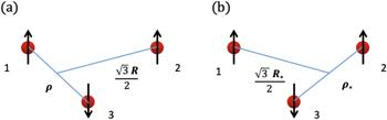
Figure 1. The three-atom system and the definitions of the Jacobi coordinates (ρ, R) (a) and (ρ*, R*) (b). |
The remainder of this paper is organized as follows. In section 2 , we show our calculation approach and derive the equation of the three-body eigen-energy. The results of our calculation are shown in section 3 . In section 4 there is a summary and some discussions.
2. Equation of energy spectrum
2.1. System and model
We consider three identical spin-1/2 ultracold fermionic atoms in 2D space, with two of them (atoms 1 and 2) being in the spin-up (↑) state and the other one (atoms 3) being in the spin-down (↓) state (figure 1). We assume these atoms are confined in a 2D anisotropic potential with confinement frequency ωx(y) along the x- (y-) direction.
For such a system, the center-of-mass motion and relative motion of three atoms are not coupled to the relative motion. In this work, we just derive the energy spectrum for the relative motion. The Hamiltonian for the relative motion of our system can be expressed as
$\begin{eqnarray}H={H}_{0}+V,\end{eqnarray}$
with H0 and V being the free Hamiltonian and the inter-atomic interaction, respectively. Explicitly, H0 can be expressed as $\begin{eqnarray}{H}_{0}={H}_{{\boldsymbol{\rho }}}+{H}_{{\boldsymbol{R}}},\end{eqnarray}$
with Hρ and HR being defined as $\begin{eqnarray}{H}_{{\boldsymbol{\rho }}}=-\displaystyle \frac{{{\hslash }}^{2}}{2\mu }{{\rm{\nabla }}}_{{\boldsymbol{\rho }}}^{2}+\displaystyle \frac{1}{2}\mu \left({\omega }_{x}^{2}{\rho }_{x}^{2}+{\omega }_{y}^{2}{\rho }_{y}^{2}\right),\end{eqnarray}$
$\begin{eqnarray}{H}_{{\boldsymbol{R}}}=-\displaystyle \frac{{{\hslash }}^{2}}{2\mu }{{\rm{\nabla }}}_{{\boldsymbol{R}}}^{2}+\displaystyle \frac{1}{2}\mu \left({\omega }_{x}^{2}{R}_{x}^{2}+{\omega }_{y}^{2}{R}_{y}^{2}\right).\end{eqnarray}$
Here ρ = (ρx, ρy) and R = (Rx, Ry) are the Jacobi coordinates which are defined as (figure 1(a)) $\begin{eqnarray}{\boldsymbol{\rho }}={{\boldsymbol{r}}}_{1}-{{\boldsymbol{r}}}_{3},\end{eqnarray}$
$\begin{eqnarray}{\boldsymbol{R}}=\displaystyle \frac{2}{\sqrt{3}}\left(\displaystyle \frac{{{\boldsymbol{r}}}_{3}+{{\boldsymbol{r}}}_{1}}{2}-{{\boldsymbol{r}}}_{2}\right),\end{eqnarray}$
where rj (j = 1, 2, 3) is the coordinate of the atom j, μ = m/2 is the two-atom reduced mass with m being the single-atom mass. Furthermore, for our system with ultracold atoms, we only consider the s-wave interaction, which occurs only between atoms in different spin states, i.e. the interaction between atoms 3 and 1 and the one between 2 and 3. Therefore, the inter-atomic interaction potential V can be formally expressed as $\begin{eqnarray}V=U({\boldsymbol{\rho }})+U({{\boldsymbol{\rho }}}_{* }).\end{eqnarray}$
As defined before, ρ is the relative coordinate of the atoms 3 and 1. In addition, ρ* is the relative coordinate of the atoms 2 and 3 (figure 1(b)), i.e. $\begin{eqnarray}{{\boldsymbol{\rho }}}_{* }\equiv {{\boldsymbol{r}}}_{2}-{{\boldsymbol{r}}}_{3}=\displaystyle \frac{1}{2}\left({\boldsymbol{\rho }}-\sqrt{3}{\boldsymbol{R}}\right).\end{eqnarray}$
2.2. Schrödinger equation and boundary conditions
In this and the next subsection, we derive the equation for the eigen-energies of our system. We begin from the eigen-equation of the total Hamiltonian H of the relative motion:2 ), (7 ), we can re-express equation (9 ) as12 ) G0 is the Green’s function with respect to the free Hamiltonian H0, which satisfies
$\begin{eqnarray}H{\rm{\Psi }}({\boldsymbol{\rho }},{\boldsymbol{R}})={E}_{b}{\rm{\Psi }}({\boldsymbol{\rho }},{\boldsymbol{R}}),\end{eqnarray}$
with Eb and $\Psi$(ρ, R) being the eigen-energy and corresponding eigen wave function, respectively. Using direct calculations with equations ( $\begin{eqnarray}\begin{array}{rcl}{\rm{\Psi }}({\boldsymbol{\rho }},{\boldsymbol{R}}) & = & \displaystyle \frac{1}{\sqrt{2}}\left\{\psi ({\boldsymbol{\rho }},{\boldsymbol{R}})-{{\mathbb{P}}}_{12}\left[\psi ({\boldsymbol{\rho }},{\boldsymbol{R}})\right]\right\}\\ & = & \displaystyle \frac{1}{\sqrt{2}}\left\{\psi ({\boldsymbol{\rho }},{\boldsymbol{R}})-\psi ({{\boldsymbol{\rho }}}_{* },{{\boldsymbol{R}}}_{* })\right\},\end{array}\end{eqnarray}$
with R* being defined as (figure 1(b)): $\begin{eqnarray}{{\boldsymbol{R}}}_{* }\equiv \displaystyle \frac{2}{\sqrt{3}}\left(\displaystyle \frac{{{\boldsymbol{r}}}_{2}+{{\boldsymbol{r}}}_{3}}{2}-{{\boldsymbol{r}}}_{1}\right)=\displaystyle \frac{1}{2}\left(-\sqrt{3}{\boldsymbol{\rho }}-{\boldsymbol{R}}\right),\end{eqnarray}$
and ψ(ρ, R) satisfying the Lippman–Schwinger-type equation: $\begin{eqnarray}{\rm{\Psi }}({\boldsymbol{\rho }},{\boldsymbol{R}})=\int {G}_{0}({E}_{b};{\boldsymbol{\rho }},{\boldsymbol{R}};{{\boldsymbol{\rho }}}^{{\prime} },{{\boldsymbol{R}}}^{{\prime} })U({{\boldsymbol{\rho }}}^{{\prime} })\psi ({{\boldsymbol{\rho }}}^{{\prime} },{{\boldsymbol{R}}}^{{\prime} }){\rm{d}}{{\boldsymbol{R}}}^{{\prime} }{\rm{d}}{{\boldsymbol{\rho }}}^{{\prime} }.\end{eqnarray}$
Here ${{\mathbb{P}}}_{12}$ is the permutation operator for r1 and r2, and we have used the fact that the wave function is anti-symmetric under this permutation. Notice that ${{\mathbb{P}}}_{12}$ is nothing but the transformation $\left\{{\boldsymbol{R}},{\boldsymbol{\rho }}\right\}\iff \left\{{{\boldsymbol{R}}}_{* },{{\boldsymbol{\rho }}}_{* }\right\}$. Moreover, in equation ( $\begin{eqnarray}\left[{E}_{b}-{H}_{0}\right]{G}_{0}({E}_{b};{\boldsymbol{\rho }},{\boldsymbol{R}};{{\boldsymbol{\rho }}}^{{\prime} },{{\boldsymbol{R}}}^{{\prime} })=\delta \left({\boldsymbol{\rho }}-{{\boldsymbol{\rho }}}^{{\prime} }\right)\delta \left({\boldsymbol{R}}-{{\boldsymbol{R}}}^{{\prime} }\right),\end{eqnarray}$
as well as the boundary conditions G0 → 0 in the limits ∣R∣ → ∞ and ∣ρ∣ → ∞.Furthermore, we use a zero-range model to describe the inter-atomic interaction in this work. Explicitly, we replace the potential U(ρ) and U(ρ*) with the 2D Bethe–Peierls boundary conditions (BPCs), i.e.10 ) is still applicable, while equation (12 ) can be simplified to28 ), (32 ) below. Substituting equation (16 ) into (10 ), we obtain
$\begin{eqnarray}\mathop{\mathrm{lim}}\limits_{| {\boldsymbol{\rho }}| \to 0}{\rm{\Psi }}({\boldsymbol{\rho }},{\boldsymbol{R}})=\left[\mathrm{ln}(| {\boldsymbol{\rho }}| )-\mathrm{ln}({a}_{2{\rm{D}}})\right]F({\boldsymbol{R}})+{ \mathcal O }(| {\boldsymbol{\rho }}| ),\end{eqnarray}$
$\begin{eqnarray}\mathop{\mathrm{lim}}\limits_{| {{\boldsymbol{\rho }}}_{* }| \to 0}{\rm{\Psi }}({\boldsymbol{\rho }},{\boldsymbol{R}})=\left[\mathrm{ln}(| {{\boldsymbol{\rho }}}_{* }| )-\mathrm{ln}({a}_{2{\rm{D}}})\right]{F}_{* }({{\boldsymbol{R}}}_{* })+{ \mathcal O }(| {{\boldsymbol{\rho }}}_{* }| ).\end{eqnarray}$
Here a2D is the 2D scattering length corresponding to the realistic interaction between two atoms with spin up and spin down, respectively, and the functions F(R) and F*(R*) should be determined by the self-consistent calculations, if it is required. In this BPC approach, the above result ( $\begin{eqnarray}{\rm{\Psi }}({\boldsymbol{\rho }},{\boldsymbol{R}})=\int {G}_{0}({E}_{b};{\boldsymbol{\rho }},{\boldsymbol{R}};{\bf{0}},{{\boldsymbol{R}}}^{{\prime} })f({{\boldsymbol{R}}}^{{\prime} }){\rm{d}}{{\boldsymbol{R}}}^{{\prime} },\end{eqnarray}$
with the function $f({{\boldsymbol{R}}}^{{\prime} })$ being determined in equations ( $\begin{eqnarray}\begin{array}{l}{\rm{\Psi }}({\boldsymbol{\rho }},{\boldsymbol{R}})=\displaystyle \frac{1}{\sqrt{2}}\left\{\displaystyle \int {G}_{0}\left({E}_{b};{\boldsymbol{\rho }},{\boldsymbol{R}};{\bf{0}},{{\boldsymbol{R}}}^{{\prime} }\right)f({{\boldsymbol{R}}}^{{\prime} }){\rm{d}}{{\boldsymbol{R}}}^{{\prime} }\right.\\ \quad \left.-\displaystyle \int {G}_{0}\left({E}_{b};{\boldsymbol{\rho }},{\boldsymbol{R}};-\displaystyle \frac{\sqrt{3}}{2}{{\boldsymbol{R}}}^{{\prime} },-\displaystyle \frac{1}{2}{{\boldsymbol{R}}}^{{\prime} }\right)f({{\boldsymbol{R}}}^{{\prime} }){\rm{d}}{{\boldsymbol{R}}}^{{\prime} }\right\}.\end{array}\end{eqnarray}$
2.3. Equation for eigen-energies
In the following, we derive the equation for the eigen-energy Eb by matching the wave function (17 ) with the BPCs of equations (14 ) and (15 ). Here we use the method of [2] in which the three-body problem in a 3D anisotropic confinement is solved.
To this end, we first study the eigen-energies and eigen-states of Hρ and HR defined in equations (3 ) (4 ). It is clear that the eigen-energies of Hρ and HR are the same, and can be denoted as En with
$\begin{eqnarray}{\boldsymbol{n}}=({n}_{x},{n}_{y}),\end{eqnarray}$
where nx(y) are the quantum numbers of the x- (y-) direction. Explicitly, we have $\begin{eqnarray}{E}_{{\boldsymbol{n}}}=\left({n}_{x}+\displaystyle \frac{1}{2}\right){\hslash }{\omega }_{x}+\left({n}_{y}+\displaystyle \frac{1}{2}\right){\hslash }{\omega }_{y}.\end{eqnarray}$
We further denote the eigen wave functions of Hρ and HR corresponding to En as φn(ρ) and φn(R), respectively. Notice that for a given quantum number n the eigen state of Hρ and HR have the same wave function and different arguments.With these notations, the three-body Green’s function G0 can be expressed as25 ), 2F1 is the Hypergeomtric function, ${\eta }_{x,y}=\tfrac{{\omega }_{x,y}}{{\omega }_{y}}$, ${\epsilon }_{{n}_{x}}=\left({n}_{x}+\tfrac{1}{2}\right){\hslash }{\omega }_{x}$ and ${C}_{{ \mathcal E }}^{(2{\rm{D}})}$ is a number set defined as
$\begin{eqnarray}\begin{array}{l}{G}_{0}({E}_{b};{\boldsymbol{\rho }},{\boldsymbol{R}};{{\boldsymbol{\rho }}}^{{\prime} },{{\boldsymbol{R}}}^{{\prime} })=\displaystyle \sum _{{\boldsymbol{n}}}{\phi }_{{\boldsymbol{n}}}^{* }({{\boldsymbol{R}}}^{{\prime} }){\phi }_{{\boldsymbol{n}}}({\boldsymbol{R}})\cdot {{ \mathcal G }}^{2{\rm{D}}}({E}_{b}-{E}_{{\boldsymbol{n}}};{\boldsymbol{\rho }},{{\boldsymbol{\rho }}}^{{\prime} }),\end{array}\end{eqnarray}$
where ${{ \mathcal G }}^{2{\rm{D}}}({ \mathcal E };{\boldsymbol{\rho }},{{\boldsymbol{\rho }}}^{{\prime} })$ is the Green’s function for the two-atom relative Hamiltonian Hρ, and which is defined as $\begin{eqnarray}{{ \mathcal G }}^{2{\rm{D}}}({ \mathcal E };{\boldsymbol{\rho }},{{\boldsymbol{\rho }}}^{{\prime} })=\sum _{\tilde{{\boldsymbol{n}}}}\displaystyle \frac{{\phi }_{\tilde{{\boldsymbol{n}}}}^{* }({{\boldsymbol{\rho }}}^{{\prime} }){\phi }_{\tilde{{\boldsymbol{n}}}}({\boldsymbol{\rho }})}{{ \mathcal E }-{E}_{\tilde{{\boldsymbol{n}}}}}.\end{eqnarray}$
Furthermore, in the previous work [43], we obtained the behavior of ${{ \mathcal G }}^{2{\rm{D}}}({ \mathcal E };{\boldsymbol{\rho }},{\bf{0}})$ in the short-range limit, i.e. $\begin{eqnarray}\mathop{\mathrm{lim}}\limits_{| {\boldsymbol{\rho }}| \to 0}\displaystyle \frac{\pi {{\hslash }}^{2}}{\mu }{{ \mathcal G }}^{2{\rm{D}}}({ \mathcal E };{\boldsymbol{\rho }},{\bf{0}})=\mathrm{ln}({\boldsymbol{\rho }})-{J}_{2{\rm{D}}}({ \mathcal E }),\end{eqnarray}$
with the function ${J}_{2{\rm{D}}}({ \mathcal E })$ being defined as: $\begin{eqnarray}\begin{array}{l}{J}_{2{\rm{D}}}({ \mathcal E })=4\pi \left[{\displaystyle \int }_{0}^{{\rm{\Lambda }}}{A}_{2{\rm{D}}}({ \mathcal E },\beta ){\rm{d}}\beta +{B}_{2{\rm{D}}}^{(1)}({ \mathcal E },{\rm{\Lambda }})\right.\\ \left.+\,{B}_{2{\rm{D}}}^{(2)}({ \mathcal E },{\rm{\Lambda }})-\displaystyle \frac{{\rm{\Gamma }}(0,\kappa {\rm{\Lambda }})}{8\pi }\right].\end{array}\end{eqnarray}$
Here Λ and κ are arbitrary finite positive numbers, and the value of ${J}_{2{\rm{D}}}({ \mathcal E })$ is independent of the values of Λ and κ, Γ[a, z] is the incomplete Gamma function, and the functions ${A}_{2{\rm{D}}}({ \mathcal E },\beta )$ and ${B}_{2{\rm{D}}}^{(1,2)}({ \mathcal E },{\rm{\Lambda }})$ are defined as $\begin{eqnarray}\begin{array}{ll}{A}_{2{\rm{D}}}({ \mathcal E },\beta )=\displaystyle \frac{{e}^{\beta { \mathcal E }}}{2}\prod _{\alpha =x,y} & \sqrt{\displaystyle \frac{{\eta }_{\alpha }}{4\pi \sinh \left({\eta }_{\alpha }\beta \right)}}-\displaystyle \frac{1}{8\pi \beta }{{\rm{e}}}^{-\kappa \beta },\end{array}\end{eqnarray}$
$\begin{eqnarray}\begin{array}{l}{B}_{2{\rm{D}}}^{(1)}({ \mathcal E },{\rm{\Lambda }})=-\displaystyle \frac{\gamma }{4\pi }-\displaystyle \frac{1}{8\pi }\mathrm{ln}\left(\displaystyle \frac{\kappa }{4}\right)\\ +\displaystyle \sum _{{n}_{x}\in {C}_{{ \mathcal E }}^{(2{\rm{D}})}}\left\{\displaystyle \frac{\sqrt{{\eta }_{x}}{2}^{{n}_{x}-3}{e}^{({ \mathcal E }-{\epsilon }_{{n}_{x}}-\tfrac{3}{2}){\rm{\Lambda }}}\sqrt{{e}^{2{\rm{\Lambda }}}-1}\cdot {\rm{\Gamma }}\left(\tfrac{1}{4}-\tfrac{{ \mathcal E }-{\epsilon }_{{n}_{x}}}{2}\right)}{{\rm{\Gamma }}{\left(\tfrac{1-{n}_{x}}{2}\right)}^{2}{\rm{\Gamma }}({n}_{x}+1){\rm{\Gamma }}\left(\tfrac{5}{4}-\tfrac{{ \mathcal E }-{\epsilon }_{{n}_{x}}}{2}\right)}\right.\\ \left.\times {\,}_{2}{{\rm{F}}}^{1}\left[1,\displaystyle \frac{3}{4}-\displaystyle \frac{{ \mathcal E }-{\epsilon }_{{n}_{x}}}{2},\displaystyle \frac{5}{4}-\displaystyle \frac{{ \mathcal E }-{\epsilon }_{{n}_{x}}}{2},{e}^{-2{\rm{\Lambda }}}\right]\right\},\end{array}\end{eqnarray}$
and $\begin{eqnarray}\begin{array}{l}{B}_{2{\rm{D}}}^{(2)}({ \mathcal E },{\rm{\Lambda }})=-\displaystyle \sum _{{n}_{x}\notin {C}_{{ \mathcal E }}^{(2{\rm{D}})}}\displaystyle \frac{{2}^{{n}_{x}-\tfrac{3}{2}}\cdot \sqrt{{\eta }_{x}\mathrm{csch}{\rm{\Lambda }}}}{{\rm{\Gamma }}{\left(\tfrac{1-{n}_{x}}{2}\right)}^{2}{\rm{\Gamma }}({n}_{x}+1)}\\ \times \,\displaystyle \frac{{e}^{({ \mathcal E }-{\epsilon }_{{n}_{x}}-2){\rm{\Lambda }}}({e}^{2{\rm{\Lambda }}}-1){\times }_{2}{{\rm{F}}}^{1}\left[1,\tfrac{3}{4}-\tfrac{{ \mathcal E }-{\epsilon }_{{n}_{x}}}{2},\tfrac{5}{4}-\tfrac{{ \mathcal E }-{\epsilon }_{{n}_{x}}}{2},{e}^{-2{\rm{\Lambda }}}\right]}{2({ \mathcal E }-{\epsilon }_{{n}_{x}})-1}.\end{array}\end{eqnarray}$
In equation ( $\begin{eqnarray}{C}_{{ \mathcal E }}^{(2{\rm{D}})}:\left\{\left.{n}_{x}\right|{n}_{x}=0,2,4,6,\,\ldots ;\,{\epsilon }_{{n}_{x}}+\displaystyle \frac{1}{2}\leqslant { \mathcal E }\right\}.\end{eqnarray}$
Substituting equation (22 ) into (20 ) and then into equation (17 ), and further expanding the function f(R) of equation (17 ) as29 ) with BPC of equation (14 ), we find that31 ) by ${\phi }_{{\boldsymbol{n}}^{\prime} }^{* }({\boldsymbol{R}})$ and integrate over R, and then derive
$\begin{eqnarray}f({\boldsymbol{R}})=\sum _{{\boldsymbol{n}}}{f}_{{\boldsymbol{n}}}{\phi }_{{\boldsymbol{n}}}({\boldsymbol{R}}),\end{eqnarray}$
we obtain $\begin{eqnarray}\begin{array}{l}\mathop{\mathrm{lim}}\limits_{| {\boldsymbol{\rho }}| \to 0}{\rm{\Psi }}({\boldsymbol{\rho }},{\boldsymbol{R}})=\displaystyle \frac{1}{\sqrt{2}}\displaystyle \sum _{{\boldsymbol{n}}}{f}_{{\boldsymbol{n}}}\\ \times \,\left[\mathop{\mathrm{lim}}\limits_{{\boldsymbol{\rho }}\to 0}{{ \mathcal G }}^{2{\rm{D}}}({E}_{b}-{E}_{{\boldsymbol{n}}};{\boldsymbol{\rho }},{\bf{0}}){\phi }_{{\boldsymbol{n}}}({\boldsymbol{R}})-{{ \mathcal G }}^{2{\rm{D}}}\right.\\ \left.\times \,\left({E}_{b}-{E}_{{\boldsymbol{n}}};-\displaystyle \frac{\sqrt{3}}{2}{\boldsymbol{R}},{\bf{0}}\right){\phi }_{{\boldsymbol{n}}}\left(-\displaystyle \frac{1}{2}{\boldsymbol{R}}\right)\right].\end{array}\end{eqnarray}$
Matching equation ( $\begin{eqnarray}F({\boldsymbol{R}})=\displaystyle \frac{\mu }{\sqrt{2}\pi {{\hslash }}^{2}}\cdot f({\boldsymbol{R}}),\end{eqnarray}$
and obtain $\begin{eqnarray}\begin{array}{l}\displaystyle \frac{1}{\sqrt{2}}\displaystyle \sum _{{\boldsymbol{n}}}{f}_{{\boldsymbol{n}}}\left[\mathop{\mathrm{lim}}\limits_{| {\boldsymbol{\rho }}| \to 0}{{ \mathcal G }}^{2{\rm{D}}}\left({E}_{b}-{E}_{{\boldsymbol{n}}};{\boldsymbol{\rho }},{\bf{0}}\right){\phi }_{{\boldsymbol{n}}}({\boldsymbol{R}})-{{ \mathcal G }}^{2{\rm{D}}}\right.\\ \left.\times \,\left({E}_{b}-{E}_{{\boldsymbol{n}}};-\displaystyle \frac{\sqrt{3}}{2}{\boldsymbol{R}},{\bf{0}}\right){\phi }_{{\boldsymbol{n}}}\left(-\displaystyle \frac{1}{2}{\boldsymbol{R}}\right)\right]\\ =\,\displaystyle \frac{\mu }{\sqrt{2}\pi {{\hslash }}^{2}}\displaystyle \sum _{{\boldsymbol{n}}}{f}_{{\boldsymbol{n}}}{\phi }_{{\boldsymbol{n}}}({\boldsymbol{R}})\left[\mathrm{ln}(\rho )-\mathrm{ln}({a}_{2{\rm{D}}})\right].\end{array}\end{eqnarray}$
We further multiply equation ( $\begin{eqnarray}\sum _{{\boldsymbol{n}}}{f}_{{\boldsymbol{n}}}{{ \mathcal M }}_{{\boldsymbol{n}},{{\boldsymbol{n}}}^{{\prime} }}({E}_{b})=0,\end{eqnarray}$
where the function ${{ \mathcal M }}_{{\boldsymbol{n}},{{\boldsymbol{n}}}^{{\prime} }}({E}_{b})$ is defined as $\begin{eqnarray}\begin{array}{l}{{ \mathcal M }}_{{\boldsymbol{n}},{{\boldsymbol{n}}}^{{\prime} }}({E}_{b})=\left\{\Space{0ex}{3.2ex}{0ex}\left[\mathrm{ln}({a}_{2{\rm{D}}})-{J}_{2{\rm{D}}}({E}_{b}-{E}_{{\boldsymbol{n}}})\right]\right.\\ \left. \times \,{\delta }_{{\boldsymbol{n}},{\boldsymbol{n}}^{\prime} }-\displaystyle \frac{\pi {{\hslash }}^{2}}{\mu }{I}_{{\boldsymbol{n}},{\boldsymbol{n}}^{\prime} }^{2{\rm{D}}}({E}_{b}-{E}_{{\boldsymbol{n}}})\right\},\end{array}\end{eqnarray}$
with $\begin{eqnarray}\begin{array}{l}{I}_{{\boldsymbol{n}},{\boldsymbol{n}}^{\prime} }^{2{\rm{D}}}({E}_{b}-{E}_{{\boldsymbol{n}}})=\displaystyle \int {{ \mathcal G }}^{2{\rm{D}}}\left({E}_{b}-{E}_{{\boldsymbol{n}}};-\displaystyle \frac{\sqrt{3}}{2}{\boldsymbol{R}},{\bf{0}}\right){\phi }_{{\boldsymbol{n}}}\left(-\displaystyle \frac{1}{2}{\boldsymbol{R}}\right) {\times \phi }_{{\boldsymbol{n}}^{\prime} }^{* }({\boldsymbol{R}}){\rm{d}}{\boldsymbol{R}}.\end{array}\end{eqnarray}$
Equation (32 ) yields that35 ) is the explicit transcendental equation of the eigen-energy Eb of the Hamiltonian H for the relative motion of these three atoms. By numerically solving equation (35 ) we can derive the energy spectrum of our system.
$\begin{eqnarray}\det \left[{ \mathcal M }({E}_{b})\right]=0,\end{eqnarray}$
where ${ \mathcal M }({E}_{b})$ is the matrix with matrix element ${{ \mathcal M }}_{{\boldsymbol{n}},{{\boldsymbol{n}}}^{{\prime} }}({E}_{b})$, where n (${{\boldsymbol{n}}}^{{\prime} }$) is the row (column) label, respectively. Equation (2.4. Confinement parity
Here we emphasize that the parities of the confinement potentials in the x- and y-directions are ‘good quantum numbers’ of our system. Explicitly, by denoting35 ) can be separated into four blocks with resecting different parities of nx,y and ${n}_{x,y}^{{\prime} }$, and thus we can solve equation (35 ) for the following four parity combinations separately:
$\begin{eqnarray}{\boldsymbol{n}}=({n}_{x},{n}_{y});\ {{\boldsymbol{n}}}^{{\prime} }=({n}_{x}^{{\prime} },{n}_{y}^{{\prime} }),\end{eqnarray}$
and denote P(n) as the parity of the integer n, we find that: $\begin{eqnarray}{{ \mathcal M }}_{{\boldsymbol{n}},{{\boldsymbol{n}}}^{{\prime} }}({E}_{b})=0\ \mathrm{for}\ {P}({n}_{x})\ne {P}({n}_{x}^{{\prime} })\ \mathrm{or}\ {P}({n}_{y})\ne {P}({n}_{y}^{{\prime} }).\end{eqnarray}$
Namely, ${{ \mathcal M }}_{{\boldsymbol{n}},{{\boldsymbol{n}}}^{{\prime} }}({E}_{b})$ is non-zero only when both ${P}({n}_{x})={P}({n}_{x}^{{\prime} })$ and ${P}({n}_{y})={P}({n}_{y}^{{\prime} })$ are satisfied. Therefore, the matrix ${ \mathcal M }({E}_{b})$ of equation ( $\begin{eqnarray*}\begin{array}{rcl}({\bf{ee}}):{P}({n}_{x}) & = & {P}({n}_{x}^{{\prime} })=\mathrm{even};\ {P}({n}_{y})={P}({n}_{y}^{{\prime} })=\mathrm{even},\\ ({\bf{eo}}):{P}({n}_{x}) & = & {P}({n}_{x}^{{\prime} })=\mathrm{even};\ {P}({n}_{y})={P}({n}_{y}^{{\prime} })=\mathrm{odd},\\ ({\bf{oe}}):{P}({n}_{x}) & = & {P}({n}_{x}^{{\prime} })=\mathrm{odd};\ {P}({n}_{y})={P}({n}_{y}^{{\prime} })=\mathrm{even},\\ ({\bf{oo}}):{P}({n}_{x}) & = & {P}({n}_{x}^{{\prime} })=\mathrm{odd};\ {P}({n}_{y})={P}({n}_{y}^{{\prime} })=\mathrm{odd}.\end{array}\end{eqnarray*}$
3. Results
In figure 2 we illustrate the energy spectrum given by the numerical solutions of equation (35 ), for the systems with the aspect ratio2.4 are displayed separately in the subfigures of figure 2.
$\begin{eqnarray}\eta \equiv \displaystyle \frac{{\omega }_{x}}{{\omega }_{y}}=1,3,6.\end{eqnarray}$
For each fixed η, the energy spectrum four parity combinations (ee), (eo), (oe) and (oo) defined in section 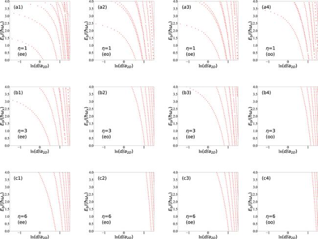
Figure 2. The energy spectra of the relative motion of three fermions in a 2D harmonic trap, for the cases with aspect ratio η = ωx/ωy = 1 ((a1)–(a4)), η = 3 ((b1)–(b4)) and η = 6 ((c1)–(c4)). For each given value of η, we show the results for the four parity combinations (ee), (eo), (oe) and (oo) defined in section |
4. Summary
In this work, we calculate the energy spectrum of three identical fermionic ultracold atoms in two different internal states in a 2D anisotropic harmonic confinement. We derive the explicit transcendental equation for the eigen-energy of the relative motion of these three atoms, i.e. equation (35 ). By numerically solving this equation, the eigen-energies can be calculated as functions of the 2D scattering length a2D between two atoms in different internal states. Our results can be used for the study of few-body dynamics or many-body properties, e.g. the calculation of the second 3rd Virial coefficients. Our method can be generalized to the three-body problems in 2D confinements of Bosonic or distinguishable atoms.