


1. Introduction
Machine learning [1] is a multi-field interdisciplinary subject, which is based on studying how computers simulate or realize human learning behavior to acquire new knowledge or skills, then reorganize the existing knowledge structure and improve its performance. There are two types of machine learning, supervised learning and unsupervised learning, the difference is whether the label is stamped in advance. A support vector machine (SVM) [1, 2] for classification is a frequently-used supervised learning algorithm. Like all machine learning algorithms, SVM is weak in facing billions and trillions of training data. Due to the exponential acceleration of quantum algorithms over classical algorithms [3, 4], a quantum support vector machine (QSVM) [5] emerges as the times require, and the experiment also proves its feasibility [6]. In the last decade, research and application of SVM has always been a hot topic, such as least squares SVM (LS-SVM) [7, 8], multi-class SVM [9–11], quantum multi-class SVM [12, 13], and twin support vector machine [14–16] etc.
In recent years, many classical algorithms that can replace quantum algorithms have been proposed, and they also achieve the exponential acceleration that quantum algorithms can achieve. Due to Tang's [17] query and challenge to quantum machine learning, many quantized versions of classical machine learning are eclipsed. Since quantum random access memory [18, 19] may be replaced by ‘sample and query access' and quantum machine learning algorithm is not accelerated in the process, hitting a number of scholars who study how to quantize classical algorithms. Before the advent of quantum computers, we could not get an accurate result from this debate. At this time, the practicability of the variational quantum algorithm shows its value. Up to now, variational quantum algorithms have been widely used and solved some problems that are beyond the power of classical computers [20–24].
The manuscript is organized as follows. We first review the SVM and QSVM algorithms and give the quantum circuit diagrams. We then propose a variational QSVM algorithm that uses the most fundamental measurement method—Hadamard Test—to complete the classification stage. Finally, the numerical experiment shows the feasibility of the algorithm.
2. Support vector machine
An SVM is used for binary classification of data, which classifies $\{({\vec{x}}_{i},{y}_{i}):{\vec{x}}_{i}\in {{\mathbb{R}}}^{N},{y}_{i}=\pm 1\}(i=1,2,\ldots ,M)$ into two classes, where yi is the label of ${\vec{x}}_{i}$. Whether yi equals +1 or −1 depends on which class ${\vec{x}}_{i}$ belongs to. For classification, two hyperplanes are found to separate the data, with no data inside. The maximum distance between hyperplanes is $2/\parallel \vec{\omega }\parallel $, where $\vec{\omega }$ is the normal vector. Generally speaking, $\vec{\omega }\cdot {\vec{x}}_{i}+b\geqslant 1$ constructs +1 class, correspondingly, $\vec{\omega }\cdot {\vec{x}}_{i}+b\leqslant -1$ constructs −1 class. Based on the above conditions, the expression of the SVM can be written as
$\begin{eqnarray}\begin{array}{l}\mathop{\min }\limits_{\omega ,b}\displaystyle \frac{1}{2}\parallel \omega {\parallel }^{2}\\ s.t.{y}_{i}(\vec{\omega }\cdot {\vec{x}}_{i}+b)\geqslant 1,i=1,2,\ldots ,M.\end{array}\end{eqnarray}$
By adding the Lagrange multiplier $\vec{\alpha }=({\alpha }_{1};{\alpha }_{2};...;{\alpha }_{N})$ to equation (1 ) and taking partial derivatives, the dual problem is obtained2 ). A binary classifier for new data $\vec{x}$ can be derived as
$\begin{eqnarray}\begin{array}{l}\mathop{\max }\limits_{}\displaystyle \sum _{i=1}^{N}{\alpha }_{i}-\displaystyle \frac{1}{2}\displaystyle \sum _{i,j=1}^{N}{\alpha }_{i}{\alpha }_{j}{y}_{i}{y}_{j}{K}_{{ij}}\\ s.t.\displaystyle \sum _{i=1}^{N}{\alpha }_{i}{y}_{i}=0,\\ {\alpha }_{i}\geqslant 0,i=1,2,\ldots ,M,\end{array}\end{eqnarray}$
where the kernel function is defined as ${K}_{{ij}}=k({x}_{i},{x}_{j})=\phi {\left({x}_{i}\right)}^{{\rm{T}}}\phi ({x}_{j})$. The Karush–Kuhn–Tucker [1] condition should be satisfied in equation ( $\begin{eqnarray*}y(\vec{x})=\mathrm{sgn}(\sum _{i=1}^{M}{\alpha }_{i}k({\vec{x}}_{i},\vec{x})+b).\end{eqnarray*}$
3. Quantum least squares support vector machine
The core idea is the least square method, which transforms the quadratic process into solving linear equations. The introduction of slack variables replaces the inequality constraint with the equality constraint
$\begin{eqnarray}\begin{array}{l}\mathop{\min }\limits_{\omega ,b,e}\displaystyle \frac{1}{2}\parallel \omega {\parallel }^{2}+\displaystyle \frac{\gamma }{2}\displaystyle \sum _{i=1}^{M}{e}_{i}^{2}\\ s.t.\quad {y}_{i}={\omega }^{{\rm{T}}}\phi ({x}_{i})\\ +b+{e}_{i},i=1,2,\ldots ,M.\end{array}\end{eqnarray}$
The slack variables ei represent the degree to which the sample does not satisfy the constraint, where user-specified γ determines the relative weight of the training error and the SVM objective. The following equation can be obtained by calculating the partial derivative of the dual Lagrange problem $\begin{eqnarray}F\left(\begin{array}{c}b\\ \vec{\alpha }\end{array}\right)=\left(\begin{array}{cc}0 & {\vec{1}}^{{\rm{T}}}\\ \vec{1} & {K}_{{ij}}+{\gamma }^{-1}I\end{array}\right)\left(\begin{array}{c}b\\ \vec{\alpha }\end{array}\right)=\left(\begin{array}{c}0\\ \vec{y}\end{array}\right).\end{eqnarray}$
Here, the matrix F is (M + 1) × (M + 1) dimensional, ${K}_{{ij}}={\vec{x}}_{i}^{{\rm{T}}}\cdot {\vec{x}}_{j}$ is a symmetric kernel matrix, $\vec{y}=({y}_{1};{y}_{2};...;{y}_{M})$, and $\vec{1}=(1;1;...;1)$. The hyperplane coefficients b and $\vec{\alpha }=({\alpha }_{1};{\alpha }_{2};...;{\alpha }_{M})$ can be optimized by solving $(b;\vec{\alpha })={F}^{-1}(0;\vec{y})$. Quantum exponential speed-up algorithms for solving linear equations have been proposed in [25].QSVM algorithms are divided into two parts: training and classification, as shown in figure 1.
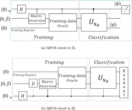
Figure 1. Brief circuit diagram of QSVM. The Matrix Inverse is employed to acquire the hyperplane parameters. The Training-data Oracle prepares ∣u⟩. The information of the query state is stored in ${U}_{{x}_{0}}$. The auxiliary qubit used to solve the equation is omitted. (a) $| \psi \rangle =\tfrac{1}{\sqrt{2}}(| 0\rangle | u\rangle +| 1\rangle | {x}_{0}\rangle )$ and $| \phi \rangle =\tfrac{1}{\sqrt{2}}(| 0\rangle -| 1\rangle )$. (b) U resets $| 0,\vec{y}\rangle $ to ∣00⟩. The QSVM algorithm in this section is based on (b). |
The quantum states are defined as
$\begin{eqnarray*}\begin{array}{l}| 0,\vec{y}\rangle =\displaystyle \frac{1}{\sqrt{{N}_{0,y}}}(| 0\rangle +\displaystyle \sum _{i=1}^{M}{y}_{i}| i\rangle ),\\ | b,\vec{\alpha }\rangle =\displaystyle \frac{1}{\sqrt{{N}_{b,\alpha }}}(b| 0\rangle +\displaystyle \sum _{i=1}^{M}{\alpha }_{i}| i\rangle ),\end{array}\end{eqnarray*}$
where N0,y = 1 + M2 and ${N}_{b,\alpha }={b}^{2}+{\sum }_{k=1}^{M}{\alpha }_{k}^{2}$ are normalization factors. Take notice that if and only if the auxiliary qubit measurement result is on ∣1⟩, the matrix inversion operation is successful. Under this condition, the training-data oracle transforms $| b,\vec{\alpha }\rangle $ to ∣u⟩, $\begin{eqnarray*}| u\rangle =\displaystyle \frac{1}{\sqrt{{N}_{u}}}(b| 0\rangle | 0\rangle +\sum _{i=1}^{M}{\alpha }_{i}| {\vec{x}}_{i}\parallel i\rangle | {\vec{x}}_{i}\rangle ),\end{eqnarray*}$
with ${N}_{u}={b}^{2}+{\sum }_{k=1}^{M}{\alpha }_{k}^{2}| {\vec{x}}_{k}{| }^{2}$.The whole process of the training section is as follows:
$\begin{eqnarray*}\begin{array}{l}| 0\rangle | 0,\vec{y}\rangle | 0\rangle \to | 0\rangle | 0,\vec{y}\rangle \displaystyle \frac{1}{\sqrt{2}}(| 0\rangle +| 1\rangle )\\ \to \displaystyle \frac{1}{\sqrt{2}}| 0\rangle | 0,\vec{y}\rangle | 1\rangle +\displaystyle \frac{1}{\sqrt{2}}| 00\rangle | 0\rangle \\ \to \displaystyle \frac{1}{\sqrt{2}}| 0\rangle | b,\vec{\alpha }\rangle | 1\rangle +\displaystyle \frac{1}{\sqrt{2}}| 00\rangle | 0\rangle \\ \to \displaystyle \frac{1}{\sqrt{2}}| u\rangle | 1\rangle +\displaystyle \frac{1}{\sqrt{2}}| 00\rangle | 0\rangle .\end{array}\end{eqnarray*}$
In the classification section, the decision function $y({\vec{x}}_{0})=\mathrm{sgn}(\langle {x}_{0}| u\rangle )$ is constructed first. The query state
$\begin{eqnarray*}| {x}_{0}\rangle =\displaystyle \frac{1}{\sqrt{{N}_{{x}_{0}}}}(| 0\rangle | 0\rangle +\sum _{i=1}^{M}| {\vec{x}}_{0}\parallel i\rangle | {\vec{x}}_{0}\rangle ),\end{eqnarray*}$
where ${N}_{{x}_{0}}=M| \vec{x}{| }^{2}+1$. When constructing the query state ∣x0⟩, ${U}_{{x}_{0}}$ needs to be introduced which transfers ∣x0⟩ to ∣00⟩, i.e., ${U}_{{x}_{0}}| {x}_{0}\rangle =| 00\rangle $.Obviously, the final state should be ∣$\Psi$⟩ = ∣φ⟩∣1⟩a +∣00⟩∣0⟩a, with $| \phi \rangle ={U}_{{x}_{0}}| u\rangle $, ∣0⟩a and ∣1⟩a are ancillary qubits. The classification result is then obtained as
$\begin{eqnarray}y({\vec{x}}_{0})=\mathrm{sgn}(\langle 00| \phi \rangle )=\mathrm{sgn}(\langle \psi | O| \psi \rangle ),\end{eqnarray}$
where $| O\rangle =| 00\rangle \langle 00| \otimes {\left(| 1\rangle \langle 0| \right)}_{a}$. If the result is greater than 0, x0 belongs to the +1 class. Otherwise, x0 belongs to the −1 class.4. Variational quantum support vector machine
In this section, we propose a variational QSVM algorithm that divides training and classification into two parts and perform a numerical simulation to verify the practicability.
4.1. Training part
The matrix F in (4 ) can be decomposed in the form of
$\begin{eqnarray}F=\sum _{i=1}^{m}{\delta }_{i}{P}_{i},\end{eqnarray}$
where $\begin{eqnarray*}{P}_{i}=\underset{\beta =1}{\overset{n}{\displaystyle \bigotimes }}{\sigma }_{t}^{\beta },\end{eqnarray*}$
t = 0, x, y, z, that is, σt is the Pauli matrix. In order to get each δi, we need to use the following formula $\begin{eqnarray*}\mathrm{Tr}[{P}_{i}F]=\mathrm{Tr}[{P}_{i}\sum _{l=0}^{m}{c}_{l}{P}_{l}]=\mathrm{Tr}[{\delta }_{i}{P}_{i}{P}_{i}]={\delta }_{i}{2}^{n}.\end{eqnarray*}$
Thus, we have $\begin{eqnarray*}{\delta }_{i}=\displaystyle \frac{\mathrm{Tr}[{P}_{i}F]}{{2}^{n}}.\end{eqnarray*}$
Of course, applying Pauli decomposition to the kernel function of a QSVM is the simplest, but it may be inefficient. Thus, we will try to find some more effective decomposition methods [26–28] to improve the feasibility of the algorithm. After the decomposition of equation (6 ) is finished, the next step is training the QSVM, and the circuit is shown in figure 2(a). Due to our choice of the Hadamard test measurement method, the loss function can be defined as follows
$\begin{eqnarray*}\begin{array}{rcl}{E}_{\mathrm{cost}} & = & 1-\displaystyle \frac{{\left(0;\vec{y}\right)}^{{\rm{T}}}F{\vec{b}}^{* }}{| (0;\vec{y})| \cdot | F{\vec{b}}^{* }| }\\ & = & 1-\displaystyle \sum _{i=1}^{m}\displaystyle \frac{{\delta }_{i}\langle 0...0| {U}_{y}{P}_{i}V(\vec{\theta })| 0...0\rangle }{| F{\vec{b}}^{* }| }\in [0,2],\end{array}\end{eqnarray*}$
where $\langle 0...0| {U}_{y}| 0,\vec{y}\rangle =1$, ${\vec{b}}^{* }=| {\rho }_{\vec{\theta }}\rangle =V(\vec{\theta })| 0...0\rangle $. The total measurement number of getting Ecost with an error ε is roughly scaling as m/ε−2 [29–31]. The gradient descent method can be selected to solve the above equation, and the descending direction is $\tfrac{\partial {E}_{\mathrm{cost}}}{\partial \vec{\theta }}$.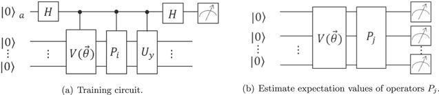
Figure 2. Brief circuit diagrams of training part of variational QSVM. (a) Calculating the molecular part of the loss function. $V(\vec{\theta })$ can be expressed as a product of L unitaries Vl(θl) sequentially acting on the input state ∣0...0⟩. As indicated, each unitary Vl(θl) can in turn be decomposed into a sequence of parametrized and unparametrized gates. Uy is a unitary matrix that satisfies $\langle 0...0| {U}_{y}=\langle 0,\vec{y}| =\tfrac{{\left(0;\vec{y}\right)}^{{\rm{T}}}}{| (0;\vec{y})| }.$ (b) Calculating the denominator of the loss function. The $\vec{\theta }$ is consistent with (a), Pj is the Pauli decomposition of F†F. Efficient derandomization Pauli measurements are employed at the end of the circuit, rather than random single-qubit measurements. |
Obviously, we have
$\begin{eqnarray*}\begin{array}{l}\left|F{\vec{b}}^{* }\right|=| {FV}(\theta )| 0...0\rangle | \\ =\sqrt{\langle 0...0| V(\vec{\theta }){F}^{\dagger }{FV}(\theta )| 0...0\rangle },\\ {F}^{\dagger }F=\displaystyle \sum _{j=1}^{m^{\prime} }{\eta }_{j}{P}_{j}.\end{array}\end{eqnarray*}$
The method of calculating $| F{\vec{b}}^{* }| $ is to estimate expectation values for the set of operators Pj in the quantum state $| {\rho }_{\vec{\theta }}\rangle $ that can be prepared repeatedly using the programmable quantum system called ansatz (shown in figure 2(b)). If all Pj have relatively low weight (the number of nonidentity tensor factors in Pj), the randomized protocol can achieve our goal quite efficiently. Because, even for sparse QSVM, the decomposition Pj of matrix F†F always has some high weight components. Thus, the derandomized Pauli measurements [32] show tremendous efficiency over randomized protocol. The derandomized protocol builds deterministic measurements one Pauli label at a time by comparing three conditional expectation values Ep[Conf(O; P)∣P#, P(k, m) = W](W = σx,y,z) (equation (6) in [32]) and then assigning the Pauli label that achieves the smallest score. Finally, the derandomized measurement P# is obtained.
Implementing the circuit in figure 2(a), we measure the probabilities of obtaining ∣0⟩ and ∣1⟩ are
$\begin{eqnarray*}\begin{array}{l}\displaystyle \frac{1}{2}(1+\langle 0...0| {U}_{y}{P}_{i}V(\vec{\theta })| 0...0\rangle ),\\ \displaystyle \frac{1}{2}(1-\langle 0...0| {U}_{y}{P}_{i}V(\vec{\theta })| 0...0\rangle ),\end{array}\end{eqnarray*}$
respectively. After M repetitions for certain i, one obtains m0 zeros and m1 ones from the measurement outcomes of the ancilla qubit. The quantities (m0 − m1)/M are an estimate of $\langle 0...0| {U}_{y}{P}_{i}V(\vec{\theta })| 0...0\rangle $. The algorithm of the training part is shown in algorithm 1. Once the algorithm terminates, it means that the training ends, then we can start the classification stage.Algorithm 1. Training variational QSVM |
| Input. An ancilla qubit initialized in $| 0\rangle $, a register initialized in $| 0...0\rangle $, a string of variable parameters $\vec{\theta }$, and set a suitable threshold ${E}_{\mathrm{cost}}^{\prime} $. |
| Step 1. Choose i = 1, repeat the circuit 2(a) M times, and record $({m}_{0}-{m}_{1})/M$. |
| Step 2. Choose j = 1, running circuit 2(b) and calculate the mean. |
| Step 3. After traversing all i and j, calculate the loss function ${E}_{\mathrm{cost}}.$ |
| Step 4. If ${E}_{\mathrm{cost}}\gt {E}_{\mathrm{cost}}^{\prime} $, update parameters $\vec{\theta }$, and then turn to Step 1; |
| else ${terminate}.$ |
4.2. Classification part
We represent the classification stage as shown in figure 3 step by step.
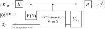
Figure 3. Brief circuit diagram of classification part of variational QSVM. The $\vec{\theta }$ of $V(\vec{\theta })$ is the one in the last cycle of algorithm 1. The Training-data Oracle prepares state ∣u⟩. ${U}_{{x}_{0}}$ contains the information of query state ∣x0⟩, and $\langle 0...0| {U}_{{x}_{0}}=\langle {x}_{0}| $. |
First, the state is initialized in
$\begin{eqnarray*}| 0{\rangle }_{a}| 0{\rangle }^{\otimes n}| 0...0\rangle .\end{eqnarray*}$
After the first Hadamard gate, we get
$\begin{eqnarray*}\displaystyle \frac{1}{\sqrt{2}}| 0{\rangle }_{a}| 0{\rangle }^{\otimes n}| 0...0\rangle +\displaystyle \frac{1}{\sqrt{2}}| 1{\rangle }_{a}| 0{\rangle }^{\otimes n}| 0...0\rangle .\end{eqnarray*}$
Then the ansatz $V(\vec{\theta })$ transforms the state to
$\begin{eqnarray*}\displaystyle \frac{1}{\sqrt{2}}| 0{\rangle }_{a}| 0{\rangle }^{\otimes n}| 0...0\rangle +\displaystyle \frac{1}{\sqrt{2}}| 1{\rangle }_{a}| b,\vec{\alpha }\rangle | 0...0\rangle .\end{eqnarray*}$
One then applies the training-data oracle to the two registers. The output state is
$\begin{eqnarray*}\displaystyle \frac{1}{\sqrt{2}}| 0{\rangle }_{a}| 0{\rangle }^{\otimes n}| 0...0\rangle +\displaystyle \frac{1}{\sqrt{2}}| 1{\rangle }_{a}| u\rangle ,\end{eqnarray*}$
where $| u\rangle =\tfrac{1}{\sqrt{{N}_{u}}}(b| 0\rangle | 0\rangle +{\sum }_{i=1}^{M}{\alpha }_{i}| {\vec{x}}_{i}\parallel i\rangle | {\vec{x}}_{i}\rangle )$, with ${N}_{u}={b}^{2}+{\sum }_{k=1}^{M}{\alpha }_{k}^{2}| {\vec{x}}_{k}{| }^{2}$.The next step is to perform ${U}_{{x}_{0}}$ construction according to query state ∣x0⟩ on the above state, the output is
$\begin{eqnarray*}\displaystyle \frac{1}{\sqrt{2}}| 0{\rangle }_{a}| 0{\rangle }^{\otimes n}| 0...0\rangle +\displaystyle \frac{1}{\sqrt{2}}| 1{\rangle }_{a}{U}_{{x}_{0}}| u\rangle .\end{eqnarray*}$
After the last Hadamard gate operating in the above state, we have the terminal state
$\begin{eqnarray*}\begin{array}{l}\displaystyle \frac{1}{2}| 0{\rangle }_{a}| 0{\rangle }^{\otimes n}| 0...0\rangle +\displaystyle \frac{1}{2}| 1{\rangle }_{a}| 0{\rangle }^{\otimes n}| 0...0\rangle \\ +\displaystyle \frac{1}{2}| 0{\rangle }_{a}{U}_{{x}_{0}}| u\rangle -\displaystyle \frac{1}{2}| 1{\rangle }_{a}{U}_{{x}_{0}}| u\rangle .\end{array}\end{eqnarray*}$
Finally, the probabilities of measuring ∣0⟩ and ∣1⟩ are
$\begin{eqnarray*}\begin{array}{l}\displaystyle \frac{1}{2}(1+\langle 0...0| {U}_{{x}_{0}}| u\rangle )=\displaystyle \frac{1}{2}(1+\langle {x}_{0}| u\rangle ),\\ \displaystyle \frac{1}{2}(1-\langle 0...0| {U}_{{x}_{0}}| u\rangle )=\displaystyle \frac{1}{2}(1-\langle {x}_{0}| u\rangle ),\end{array}\end{eqnarray*}$
respectively. Similarly, we can repeat this line T times and get t0 zeros and t1 ones. If t0 > t1, the classification result will be positive; otherwise, it will be negative. At this point, the algorithm ends.In the classification stage, we do not need to calculate the exact value of ⟨x0∣u⟩, we just need to know whether it is positive or negative. In other words, we just need to compare the size of t0 and t1. As mentioned above, estimating the value of ⟨x0∣u⟩ with an error ε demands measurements ε−2 times
$\begin{eqnarray*}| \langle {x}_{0}| u\rangle -\displaystyle \frac{{t}_{0}-{t}_{1}}{T}| \lt \epsilon .\end{eqnarray*}$
The fault tolerance classification result will be revealed by
$\begin{eqnarray}\mathrm{sgn}\left(\displaystyle \frac{{t}_{0}-{t}_{1}}{T},-,\epsilon \right)=1,\end{eqnarray}$
$\begin{eqnarray}\mathrm{sgn}\left(\displaystyle \frac{{t}_{0}-{t}_{1}}{T},+,\epsilon \right)=-1.\end{eqnarray}$
In order to improve the classification efficiency, we set two thresholds ε = 0.1, 0.01, and the detailed process of the algorithm is shown in algorithm 2.
Algorithm 2. Classification variational QSVM |
| Input. An ancilla qubit initialized in $| 0\rangle $, a register initialized in $| 0{\rangle }^{\otimes n}$, a training register initialized in $| 0...0\rangle $, construct ${U}_{{x}_{0}}$ according to query qubit $| {x}_{0}\rangle $. |
| Step 1. Set $\epsilon =0.1$, repeat the circuit ${\epsilon }^{-2}$ times. If the calculation result satisfies equations ( |
| or ( |
| Step 2. Set $\epsilon =0.01$, repeat the circuit ${\epsilon }^{-2}$ times. If the calculation result satisfies equations ( |
| or ( |
| Step 3. Erase ε in equations ( |
4.3. Numerical experiment simulation
In order to certificate the feasibility of the algorithm and its advantageous aspects over the conventional QSVM, we devise numerical experiments to test and verify it. For convenience, we quote the experimental data of [6]. Besides, to keep consistent with this, we discard the offset term b and take $F^{\prime} =K/\mathrm{tr}K$. According to the data in figure 4(a), one educes
$\begin{eqnarray}\begin{array}{l}F^{\prime} \vec{x}=\left(\begin{array}{cc}0.50 & 0.25\\ 0.25 & 0.50\end{array}\right)\left(\begin{array}{c}{x}_{1}\\ {x}_{2}\end{array}\right)\\ \,=\,\left(\displaystyle \frac{1}{2}I+\displaystyle \frac{1}{4}X\right)\left(\begin{array}{c}{x}_{1}\\ {x}_{2}\end{array}\right)\,=\,\left(\begin{array}{c}\displaystyle \frac{1}{\sqrt{2}}\\ -\displaystyle \frac{1}{\sqrt{2}}\end{array}\right)\,=\,\vec{y}.\end{array}\end{eqnarray}$
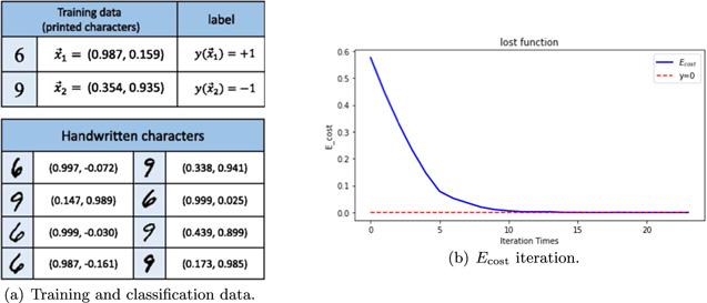
Figure 4. (a) Experimental data of [6], where the feature values are chosen as the vertical ratio and the horizontal ratio. The training data is in a standard font (Times New Roman). The arbitrary chosen handwritten samples for classification and their feature vectors. (b) Loss function image optimized by gradient descent penalty. The calculation result is simulated by Python. |
The unitary matrix Uy in figure 2(a) encoding $\vec{y}$ can be written as
$\begin{eqnarray*}{U}_{y}={R}_{y}\left(-\displaystyle \frac{\pi }{2}\right)=\left(\begin{array}{cc}\displaystyle \frac{1}{\sqrt{2}} & -\displaystyle \frac{1}{\sqrt{2}}\\ \displaystyle \frac{1}{\sqrt{2}} & \displaystyle \frac{1}{\sqrt{2}}\end{array}\right).\end{eqnarray*}$
To get the mean of $| F^{\prime} {b}^{* }| $, we have
$\begin{eqnarray*}F{{\prime} }^{\dagger }F^{\prime} =\left(\begin{array}{cc}0.31 & 0.25\\ 0.25 & 0.31\end{array}\right)=\displaystyle \frac{5}{16}I+\displaystyle \frac{1}{4}X.\end{eqnarray*}$
The correspondingly derandomized Pauli measurements are Z and X. Here, the Pauli Z measurement could substitute for Pauli X measurements by adding a Hadamard gate to the final states. In addition, the gradient of θ is
$\begin{eqnarray*}\cos (\theta /2)+\sin (\theta /2).\end{eqnarray*}$
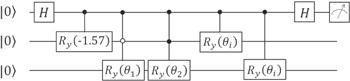
After all the preparations are ready, we conduct numerical simulation, and the iterative line chart is shown in figure 4(b). Then we construct the classification circuit shown in figure 5, where the hardware efficient ansatz with θ = −1.57 will be the subsequent classification operation as a subroutine.
Figure 5. The classification circuit. The rotation angles ${\theta }_{1}=2\arctan \tfrac{{\left({x}_{1}\right)}_{2}}{{\left({x}_{1}\right)}_{1}}$, ${\theta }_{2}=2\arctan \tfrac{{\left({x}_{2}\right)}_{2}}{{\left({x}_{2}\right)}_{1}}$. The last two controlled Ry(θi) gates form ${U}_{{x}_{0}}$, with ${\theta }_{i}=-2\arctan \tfrac{{\left({x}_{i}\right)}_{2}}{{\left({x}_{i}\right)}_{1}}$, i = 3, 4,…,10. |
We implement this task on today's current state-of-the-art quantum computer using the IBM quantum experience platform where the experimental circuit diagram and experimental results are shown in figures A1 and A2 in the appendix. For comparison, but due to the limitation of qubits, we only give the experimental circuit diagram of applying the HHL algorithm to the QSVM (shown in appendix figure A3). The results of classification results are shown in table 1. It can be seen that by adding the fault-tolerant classification formula, we can predict the results 100% accurately when we measure only 100 times.
Table 1. The classification results of samples. In the two columns below the number of measurements, the left one is the number of times the auxiliary qubit measures 0 and the right is obtaining 1. |
| Samples\Times&Results | 100 | R | 10000 | R | ||
|---|---|---|---|---|---|---|
| x3 = (0.997, − 0.072) | 73 | 27 | 6 | 6405 | 3695 | 6 |
| x4 = (0.147, 0.989) | 22 | 78 | 9 | 3636 | 6364 | 9 |
| x5 = (0.999, − 0.030) | 82 | 18 | 6 | 7466 | 2534 | 6 |
| x6 = (0.987, − 0.161) | 68 | 32 | 6 | 7540 | 2460 | 6 |
| x7 = (0.338, 0.941) | 37 | 63 | 9 | 4048 | 5952 | 9 |
| x8 = (0.999, 0.025) | 62 | 38 | 6 | 6924 | 3076 | 6 |
| x9 = (0.439, 0.899) | 36 | 64 | 9 | 4562 | 5438 | 9 |
| x10 = (0.173, 0.985) | 30 | 70 | 9 | 4524 | 5476 | 9 |
4.4. Advantage analysis
The QSVMs shown in figure 1 have put training and classification in a circuit which means that they run the whole route every time one classifies a new data. Once the classification data is much larger than the training data, the algorithms will lead to a lot of redundant operations. In practice, the long line of figure 1(a) and the complex measurement mode of figure 1(b) will be an obstacle to the successful implementation of the algorithm. Since the variational QSVM divides training and classification into two parts, when the training stage is completed, and it will turn to the classification circuit. When classifying, our algorithm only requires Hadamard test measurements and owns a shorter line depth, which is more amenable to execution on near-term devices.
Here, we analyze the circuit depth and qubits numbers of our algorithm compared with the algorithm in [5]. Our algorithm needs 2, 1 and 3 qubits, respectively, in solving equations part, calculating modules part and classifying parts. In contrast, if one adopts the HHL algorithm directly to the QSVM, there must be 4 qubits—1 ancilla qubit(abbreviated a1), 2 register qubits, and 1 qubit storing the input message and output result—in the stage of solving equations. Meanwhile, in constructing the state $| \psi \rangle =\tfrac{1}{\sqrt{2}}(| 0\rangle | u\rangle +| 1\rangle | {x}_{0}\rangle )$, there must be 1 more ancilla qubit(abbreviated a2) and 1 register qubit for building ∣u⟩ according to the output of the HHL algorithm. The total qubits number of applying the HHL algorithm to the QSVM is 6.
When applying the HHL algorithm to equation (9 ), we have to use 2 qubits for the register, despite the fact that the more registered qubits the more accurate result, and the fewer registered qubits the easier the quantum circuit. In the phase estimation stage, if we only use 1 registered qubit, the estimated eigenvalue of $F^{\prime} $ is either 0 or $\tfrac{1}{2}$ which leads to a great error. Although 3 registered qubits could estimate the eigenvalue among $\tfrac{i}{8}$, i = 0, 1,…,7, it will bring a great burden on the construction of quantum circuits. Besides, the addition of a2 produces a number of C2(U) gates which can be decomposed into 5 universal quantum gates. Thus, the circuit is much deeper than the variational QSVM circuit. Furthermore, the quantum circuit is implemented successfully under the circumstances a1 measures 1 which means that the run times exceed the variational QSVM circuit.
In a more general sense, suppose the dimension of $F^{\prime} $ is N × N, one applies the HHL algorithm to the QSVM demands at least $3+3\mathrm{log}N$ qubits overall. The corresponding part of the variational QSVM needs $1+\mathrm{log}N$, $\mathrm{log}N$ and $1+2\mathrm{log}N$ qubits, gathered $2+4\mathrm{log}N$. It can be seen that with the increase of N, the number of qubits required by applying the HHL algorithm to the QSVM is less than that of the variational QSVM. However, the number of qubits used in the phase estimation stage $1+\mathrm{log}N$ is only the minimum number we assume, and the accuracy cannot be guaranteed. Meanwhile, our algorithm shows great advantages in the depth of quantum circuits.
5. Conclusion and outlook
We propose a quantum–classical variational algorithm to solve the QSVM based on the Hadamard test and construct a loss function that is only suitable for vectors' own equal module length. That is, it applies to quantum states. Besides, our algorithm adopts the derandomization Pauli measurements protocol which shows strong advantages over random Pauli measurements due to the high weight decomposition. We have carried out simulated quantum experiments to prove the feasibility of the algorithm. In the future, we will also consider applying this algorithm to a multi-classification QSVM.