This study scrutinizes the flow of engine oil-based suspended carbon nanotubes magneto-hydrodynamics (MHD) hybrid nanofluid with dust particles over a thin moving needle following the Xue model. The analysis also incorporates the effects of variable viscosity with Hall current. For heat transfer analysis, the effects of the Cattaneo-Christov theory and heat generation/absorption with thermal slip are integrated into the temperature equation. The Tiwari-Das nanofluid model is used to develop the envisioned mathematical model. Using similarity transformation, the governing equations for the flow are translated into ordinary differential equations. The bvp4c method based on Runge-Kutta is used, along with a shooting approach. Graphs are used to examine and depict the consequences of significant parameters on involved profiles. The results revealed that the temperature of the fluid and boundary layer thickness is diminished as the solid volume fraction is raised. Also, with an enhancement in the variable viscosity parameter, the velocity distribution becomes more pronounced. The results are substantiated by assessing them with an available study.
Muhammad Ramzan, Hammad Alotaibi. Variable viscosity effects on the flow of MHD hybrid nanofluid containing dust particles over a needle with Hall current—a Xue model exploration[J]. Communications in Theoretical Physics, 2022, 74(5): 055801. DOI: 10.1088/1572-9494/ac64f2
Nomenclature
${E}_{c}$ $\qquad\qquad$ Eckert number
${m}_{d}$ $\qquad\qquad$ Dust particles mass concentration $\left(\mu {\rm{g}}\,{{\rm{m}}}^{-3}\right)$
$N$ $\qquad\qquad$ Density of dust particles $\left({\rm{g}}\,{{\rm{cm}}}^{-2}\right)$
The use of liquid flow for cooling in a range of applications for instance automobiles, metallic plate cooling, and electronics has gained great popularity. In all of these cooling systems, various convectional fluids such as water, ethylene glycol, water mixtures, and other basic fluids are exercised as coolants. Several researchers have made significant contributions to improving the thermal conductivity of coolants for many years. Choi and Eastman [1] proposed the utilization of nanoparticles to increase the thermal conductivity of base liquids. Nanofluids are essentially a mixture of solid nanoparticles and liquid coolants that have been combined. The introduction of this new kind of coolant completely transformed the current manufacturing world. The ability of nanoparticles to enrich the heat transfer phenomena of the base fluid is quite remarkable. Many studies followed up on the pioneering work of Choi and Eastman [1] by looking into the impression of putting different solid nanoparticles into a variety of working fluids along with different geometries and finding interesting results [2-6]. The cutting-edge nanofluid, ‘hybrid nanofluid,' has recently been the subject of several discreet research using two kinds of nanoparticles submerged in a base fluid. To maximize the heat transfer rate of a hybrid nanofluid, a proper combination of nanoparticles must be used. Hybrid nanofluids have a wide variety of applications in medical, lubricating, solar heating, microfluidics, nuclear system and cooling, and thermal management of vehicles. In comparison to ordinary nanofluid, the hybrid nanofluid is more efficient as a cooling agent. The concept of a hybrid nanofluid is discussed in several scholarly works. Waini et al [7] demonstrated the flow of the hybrid nanofluid with (PHF) prescribed heat flux over a thin needle erected vertically. It is noticed that rising the volume fraction of copper (Cu) nanoparticles and lowering the needle size results in a rise in the skin friction coefficient and the heat flux rate on the needle. Additionally, Sulochana et al [8] scrutinized the Al-Cu/menthol flow of the nanofluid (hybrid) across a thin needle with (thermal) radiation effects. It is discovered that increasing the needle thickness has a substantial effect on the heat transfer rate of hybrid nanoliquid. Mousavi et al [9] established the hybrid nanofluid flow comprising TiO2-Cu/H2O along a thin needle accompanying the radiation effects. The results reveal that dual solutions exist for the reverse direction of the free stream of the thin needle. Ramesh et al [10] deliberated the heat transmission of a hybrid liquid across a thin needle in a spongy medium with different effects. Further literature on hybrid nanofluids is available in the [11-18].
It is well established that heat transfer happens between two bodies or inside the same body as a result of a temperature difference. Heat transfer is a tremendously important phenomenon in industrial, technical, and biological applications. Fourier was the first to explain the heat transmission process [19]. However, it has the drawback of producing a parabolic energy equation for the temperature distribution. Cattaneo [20] solved this problem by adding the thermal relaxation period to the basic Fourier formula of heat conduction. Finally, Christov [21] replaced the Cattaneo law with an Oldroyd upper convected derivative in the Maxwell-Cattaneo model to preserve the formulation's material invariance. Cattaneo-Christov (C-C) heat flux model consistency concerns have been examined by Ciarletta and Straughan [22] in both specific and systematic approaches. The latest research has highlighted the significance of the C-C heat flux in varied models [23-27].
Numerous researchers have devoted years to studying the heat transfer properties of dusty fluid flow, which is a two-phase fluid, to better understand a variety of real-world challenges, particularly in the meteorological, medical, and engineering domains. Dust particles are employed in a diverse application, including the petroleum industry, soil erosion caused by natural winds, crude oil purification, aerosol and fluidization, paint spraying, dust entrainment after nuclear explosions in clouds, and wastewater management [28-30]. Saffman [31] developed the first dusty fluid flow equations and analyzed the stability of the laminar flow of a dusty gas with equally distributed particles. Later, Chakrabarti [32] studied dusty gas utilizing boundary layer theory. Numerous scholars have since worked on dusty fluid flow on different geometries. Recently, Kumar et al [33] considered the flow of suspended carbon nanotubes (CNTs) in a dusty nanofluid across a stretched porous rotating disk. The results indicate that SWCNT-water-based fluid exhibits a higher rate of heat transfer than MWCNTs water-based fluid in both the dust and fluid phases. Gireesha et al [34] used numerical simulations to investigate the significance of nonlinear thermal radiation and hall currents on a dusty fluid on a heated stretched sheet, whereas Abbas et al [35] investigated dusty fluid flow in a spongy media while taking slip and MHD into account. More work on dust phase fluid can be found in [36-39].
The main contribution of this investigation is to deal with the MHD nanofluid flow with CNTs in engine oil with thermal slip across a thin moving needle in two dimensions. Dust particles are also studied concerning Hall current and varying viscosity. C-C theory and heat generation/absorption are also cogitated in the temperature equation for heat transfer analysis. CNTs-based hybrid nanofluid's thermal conductivity is analyzed using a new model named the Xue model. Using the relevant similarity transformations, the resultant system of a highly nonlinear system is numerically resolved. The findings are presented using graphs. The leading objective of the present exploration is to look for the answers to the ensuing questions:
•
What are the consequences of solid volume fraction on the dust and hybrid nanofluid phases?
•
How does solid volume fraction affect the temperature of the hybrid nanofluid and dust phases?
•
What is the impact of fluid particles' interaction parameters on the fluid velocity and dust phases?
•
How hybrid nanofluid particle interaction parameter affects the fluid and dust phases?
•
What is the consequence of the Eckert number on the fluid temperature?
Mathematical modeling
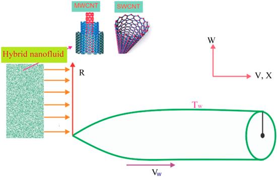
We consider a hybrid nanofluid flow past a moving needle with temperature-dependent viscosity (figure 1). The Xue model is adopted with single-wall and multi-wall CNTs immersed into the engine oil (base fluid). The radius of the cylindrical needle is presumed as $R=r(X).$ Here, the needle's leading edge is along the X-axis and $R,X$ are assumed as the radial and axial coordinates. Here, the transverse curvature is considered nevertheless the pressure gradient in the body direction is ignored. The wall temperature ${T}_{w}$ and the temperature far away from the wall ${T}_{\infty }$ are taken as constant with ${T}_{w}\gt {T}_{\infty }.$ The movement of the needle is observed with a constant velocity ${V}_{w}.$
The variable viscosity, thermal conductivity, density, and specific heat for SWCNTs/engine oil (nanofluid) and SWCNTs-MWCNTs/engine oil (hybrid nanofluid) are specified as [44, 45]:
The solid volume fraction of SWCNTs is denoted by ${\phi }_{2}$ and that of the MWCNTs is clarified by ${\phi }_{1},$ specific heat and thermal conductivity of regular fluid are correspondingly defined by ${C}_{p}$ and ${k}_{f}.$
${R}{{e}}_{{X}}=\tfrac{X{V}_{0}}{{\nu }_{f}},$ represents the local Reynold number.
Numerical appraisal
By implementing the Runge-Kutta-based MATLAB function bvp4c, the existing problem solution is found numerically. In addition, we ‘shoot' directions in this method in different ways until we have the appropriate boundary value. This is a technique that is very simple and effective. We take the convergence criterion to reach the solution, which is ${10}^{-5}.$ The solution is achieved graphically concerning different variables for the velocity and temperature for both the fluid phase and the dust phase.
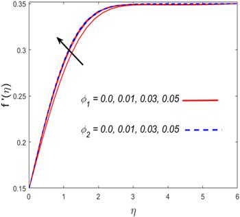
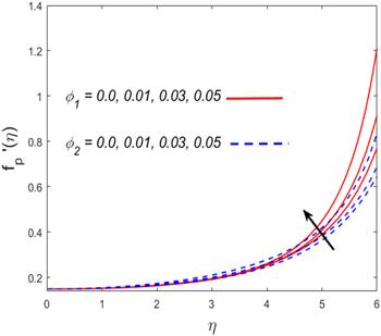
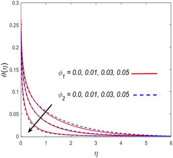
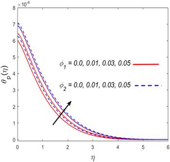
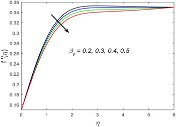
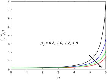
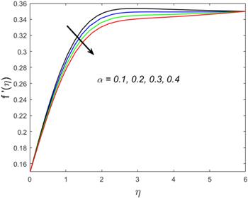
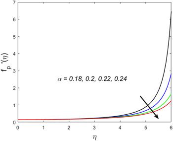
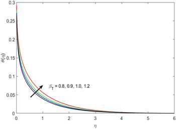
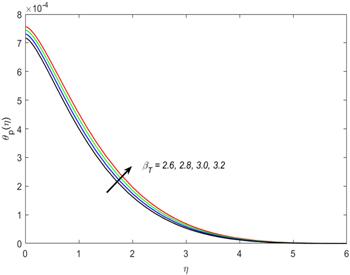
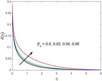
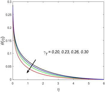
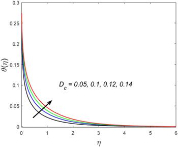
This section describes the salient parameters' correlation with the associated profiles. The values of the involved parameters are taken as: $m=2,\,{\theta }_{r}=0.1,\,{\beta }_{v}=0.3,$ $\alpha =0.2,\,{\gamma }_{T}=0.5,\,\delta =0.1,$ $\lambda =0.2,\,M=0.2,\,{\Pr }=6.2,$ ${\beta }_{T}=3,\,{E}_{c}=0.01,$ ${D}_{c}=0.1,\,c=\mathrm{0.01.}$ Figures 2-5 demonstrate the significance of solid volume fraction of SWCNTs and MWCNTs on velocity and temperature fields of fluid and dust phase. Figures 2 and 3 scrutinized the impact of solid volume fraction on velocity distribution for fluid and dust phases. It is found that the velocity of the fluid and dust phases is enhanced with an increase in the solid volume fraction. The thermal conductivity of the fluid is directly proportionate with the volume fraction that improves the fluid velocity for both fluid and dust phases. Nevertheless, the temperature profile and its related boundary layer thickness diminish for enlarged estimation of solid volume fraction (see in figure 4). While the dust phase temperature and their accompanying boundary layer thickness are enhanced (figure 5). To identify the influence of fluid particles' interaction parameter ${\beta }_{v}$ on both velocities figures 6 and 7 are sketched. It is seen that both the velocities are diminished for ${\beta }_{v}.$ This is owing to intensified fluid particles interaction that creates an opposing force to the fluid flow. This phenomenon continues till the dust phase fluid velocity accesses the fluid phase velocity. That is why declined velocities are seen here. Figures 8 and 9 are plotted for both velocity profiles for varied values of dust particles mass concentration $\alpha .$ Velocity distribution for both fluid and dust phase reduces for enlarged values of $\alpha .$ The accumulation of the dust particles into the fluid strengthens the surface drag force that eventually resists the fluid motion. That is why diminished velocities for both phases are observed. The temperature of the fluid and dust phase is an escalating function of the fluid particle interaction parameter ${\beta }_{T}$ (figures 10 and 11). It is understood from the figures that increasing values of ${\beta }_{T}$ simmer down the fluid. Thus, ${\beta }_{T}$ acts as a controlling agent for the flow behavior. The influence of the Eckert number ${E}_{c}$ on the fluid temperature is exhibited in figure 12. It is concluded that the temperature profile enhances for significant estimates of ${E}_{c}.$ The physical explanation for this outcome is an improvement in kinetic energy and the collision among nanofluid molecules because of its direct association with the Eckert number. Figure 13 examines the impact of the thermal relaxation parameter ${\gamma }_{T}$ on the temperature field. It is comprehended that the temperature of the fluid is on the decline for numerous values of ${\gamma }_{T}.$ Higher estimates of the ${\gamma }_{T}$ specify the qualities of the insulating material that lowers the fluid temperature. That is why we see a diminishing thermal profile. Figure 14 highlighted the impression of the heat generation parameter ${D}_{c}$ on the temperature profile. It is inspected that the temperature and its correlated thermal boundary layer thickness enhance with the large estimation of heat generation parameter. It is because excessive energy is produced for large estimates of heat generation that eventually boosts the fluid temperature.
Figure 14. Association of ${D}_{c}$ and temperature field $\theta (\eta ).$
Table 2 demonstrates the surface drag coefficient for numerous values of varied parameters. It is demonstrated that the drag coefficient augments with higher the estimation of solid volume fraction and variable viscosity parameter while its declines with higher the estimation of Hall current parameter, fluid particles interaction parameter, and volume fraction of dust particles.
Table 2. Numerical calculations of skin friction when ${\Pr }=6.2,\,M=0.2,\,{\phi }_{1}=0\mathrm{.03},\,\alpha =0.2.$
${\phi }_{2}$
${\theta }_{r}$
${\beta }_{v}$
${\phi }_{d}$
$m$
$R{e}_{X}^{1/2}{C}_{fX}$
0.01
0.2
0.1
0.1
1.8
1.311 023
0.03
1.322 021
0.05
1.333 654
0.3
1.130 921
0.4
1.178 143
0.5
1.223 835
0.2
1.157 031
0.3
1.147 021
0.4
1.135 022
0.2
1.117 345
0.3
1.090 334
0.4
1.063 461
1.0
1.144 932
1.5
1.132 522
2.0
1.120 150
The current result shows good accord with earlier published findings Ishak et al [40], Afridi et al [41], and Tlili et al [42] (see in table 3).
Table 3. Verification of the current problem for the varied values of c where ${\phi }_{i,d}=0=\lambda ={\beta }_{v}=m=M$ with Ishak et al [40], Afridi et al [41], and Tlili et al [42].
This research has been established to explore the impact of the magnetohydrodynamics (MHD) 2D, nanoliquid flow of engine oil as a working fluid. CNTs were inserted with thermal slip over a thin moving needle following Xue model. Variable viscosity and thermal C-C heat flux and the heat generation/absorption were supported by the thermal slip. The constructed model has been numerically handled using the bvp4c function of MATLAB software. The corresponding profiles are plotted against their relevant parameters and the findings are described coherently. The following are the most significant outcomes:
•
The fluid phase and dust phase velocities are boosted as the estimates of solid volume fraction increase.
•
For larger solid volume fraction estimation, temperature distribution and boundary layer thickness dwindled, while dust phase temperature raised.
•
The fluid and dust phases velocities have dwindled for the improved fluid particles interaction parameter.
•
Velocity distribution for fluid and dust phase reduces for enlarged values of dust particles mass concentration.
•
The temperature distribution heightens for greater estimates of the Eckert number.
The authors are thankful for the Taif University research supporting project number (TURSP-2020/304), Taif University, Saudi Arabia.
The authors declare that they have no known competing financial interests or personal relationships that could have appeared to influence the work reported in this paper.
MR supervised and conceived the idea; HA wrote the manuscript.
ChoiS UEastmanJ A1995Enhancing Thermal Conductivity of Fluids with Nanoparticles (No. ANL/MSD/CP-84938; CONF-951135-29) IL (United States) Argonne National Lab.
2
ZhangYShahmirNRamzanMAlotaibiHAljohaniH M2021 Upshot of melting heat transfer in a Von Karman rotating flow of gold-silver/engine oil hybrid nanofluid with Cattaneo-Christov heat flux Case Stud. Therm. Eng.26 101149
KhanAKumamWKhanISaeedAGulTKumamPAliI2021 Chemically reactive nanofluid flow past a thin moving needle with viscous dissipation, magnetic effects and Hall current PLoS One16 e0249264
RamzanMGulHKadrySLimCNamYHowariF2019 Impact of nonlinear chemical reaction and melting heat transfer on an MHD nanofluid flow over a thin needle in porous media Appl. Sci.9 5492
WainiIIshakAPopI2020 Dufour and Soret effects on Al2O3-water nanofluid flow over a moving thin needle: Tiwari and Das model Int. J. Numer. Methods Heat Fluid Flow31 766 782
7
WainiIIshakAPopI2019 Hybrid nanofluid flow and heat transfer past a vertical thin needle with prescribed surface heat flux Int. J. Numer. Methods Heat Fluid Flow24 4875 94
SulochanaCAparnaS RSandeepN2020 Impact of linear/nonlinear radiation on incessantly moving thin needle in MHD quiescent Al-Cu/methanol hybrid nanofluid Int. J. Ambient Energy 1 7
MousaviS MRostamiM NYousefiMDinarvandS2021 Dual solutions for MHD flow of a water-based TiO2-Cu hybrid nanofluid over a continuously moving thin needle in presence of thermal radiation Rep. Mech. Eng.2 31 40
RameshG KShehzadS AIzadiM2020 Thermal transport of hybrid liquid over thin needle with heat sink/source and Darcy-Forchheimer porous medium aspects Arab. J. Sci. Eng.45 9569 9578
ZaydanMWakifAAnimasaunI LKhanUBaleanuDSehaquiR2020 Significances of blowing and suction processes on the occurrence of thermo-magneto-convection phenomenon in a narrow nanofluidic medium: a revised Buongiorno's nanofluid model Case Stud. Therm. Eng.22 100726
RasoolGWakifA2021 Numerical spectral examination of EMHD mixed convective flow of second-grade nanofluid towards a vertical Riga plate using an advanced version of the revised Buongiorno's nanofluid model J. Therm. Anal. Calorim.143 2379 2393
UpretiHPandeyA KKumarM2021 Assessment of entropy generation and heat transfer in three-dimensional hybrid nanofluids flow due to convective surface and base fluids J. Porous Media24 35 50
BilalSShahI ARamzanMNisarK SElfasakhanyAEedE MGhazwaniH A S2022 Significance of induced hybridized metallic and non-metallic nanoparticles in single-phase nano liquid flow between permeable disks by analyzing shape factor Sci. Rep.12 1 16
SinghKPandeyA KKumarM2021 Numerical solution of micropolar fluid flow via stretchable surface with chemical reaction and melting heat transfer using Keller-Box method Propulsion Power Res.10 194 207
UpretiHPandeyA KRawatS KKumarM2021 Modified Arrhenius and thermal radiation effects on three-dimensional magnetohydrodynamic flow of carbon nanotubes nanofluids over bi-directional stretchable surface J. Nanofluids10 538 551
HudaN UHamidAKhanM2020 Impact of Cattaneo-Christov model on Darcy-Forchheimer flow of ethylene glycol base fluid over a moving needle J. Mater. Res. Technol.9 4139 4146
ReddyM GKumariP VReddyG UKumarK GPrasannakumaraB C2020 A mathematical framework on Cattaneo-Christov model over an incessant moving needle Multidiscipline Model. Mater. Struct.17 167 80
LvY PGulHRamzanMChungJ DBilalM2021 Bioconvective Reiner-Rivlin nanofluid flow over a rotating disk with Cattaneo-Christov flow heat flux and entropy generation analysis Sci. Rep.11 1 18
AnuarN SBachokNPopI2021 Numerical computation of dusty hybrid nanofluid flow and heat transfer over a deformable sheet with slip effect Mathematics9 643
ShaheenNRamzanMAlshehriAShahZKumamP2021 Soret-Dufour impact on a three-dimensional Casson nanofluid flow with dust particles and variable characteristics in a permeable media Sci. Rep.11 1 21
Naveen KumarRMallikarjunaH BTigalappaNPunith GowdaR JUmrao SarweD2021 Carbon nanotubes suspended dusty nanofluid flow over stretching porous rotating disk with non-uniform heat source/sink Int. J. Comput. Methods Eng. Sci. Mech.23 1 10
34
GireeshaB JMahantheshBMakindeO DMuhammadT2018 Effects of Hall current on transient flow of dusty fluid with nonlinear radiation past a convectively heated stretching plate Defect Diffus. Forum387 352 363
35
AbbasZHasnainJSajidM2019 Effects of slip on MHD flow of a dusty fluid over a stretching sheet through porous space J. Eng. Thermophys.28 84 102
RamzanMShaheenNChungJ DKadrySChuY MHowariF2021 Impact of Newtonian heating and Fourier and Fick's laws on a magnetohydrodynamic dusty Casson nanofluid flow with variable heat source/sink over a stretching cylinder Sci. Rep.11 1 19
BilalMRamzanM2019 Hall current effect on unsteady rotational flow of carbon nanotubes with dust particles and nonlinear thermal radiation in Darcy-Forchheimer porous media J. Therm. Anal. Calorim.138 3127 3137
MallikarjunaH BNirmalaTPunith GowdaR JManghatRVarun KumarR S2021 Two‐dimensional Darcy-Forchheimer flow of a dusty hybrid nanofluid over a stretching sheet with viscous dissipation Heat Transfer50 3934 3947
AfridiM ITliliIQasimMKhanI2018 Nonlinear Rosseland thermal radiation and energy dissipation effects on entropy generation in CNTs suspended nanofluids flow over a thin needle Boundary Value Probl.2018 1 14
TliliIRamzanMKadrySKimH WNamY2020 Radiative MHD nanofluid flow over a moving thin needle with entropy generation in a porous medium with dust particles and Hall current Entropy22 354
RamzanMGulHMalikM YBaleanuDNisarK S2021 On hybrid nanofluid Yamada-Ota and Xue flow models in a rotating channel with modified Fourier law Sci. Rep.11 1 19
RiasatSRamzanMSunY LMalikM YChinramR2021 Comparative analysis of Yamada-Ota and Xue models for hybrid nanofluid flow amid two concentric spinning disks with variable thermophysical characteristics Case Stud. Therm. Eng.26 101039


