


1. Introduction
2. A discrete hierarchy related to equation (5 )
| I | (I)When m = 1, equation ( $\begin{eqnarray}{u}_{n,{t}_{1}}=2{u}_{n}{A}_{n+1}^{(1)}-{C}_{n+1}^{(2)}={u}_{n}^{2}({u}_{n+1}-{u}_{n-1}),\end{eqnarray}$ which is the same as equation ( $\begin{eqnarray}{\phi }_{n,{t}_{1}}={V}_{n}^{(1)}{\phi }_{n}=\left(\begin{array}{cc}\displaystyle \frac{{\lambda }^{2}}{2}+{u}_{n}{u}_{n-1} & -\lambda {u}_{n}\\ \lambda {u}_{n-1} & -\displaystyle \frac{{\lambda }^{2}}{2}+{u}_{n}{u}_{n-1}\end{array}\right){\phi }_{n}.\end{eqnarray}$ However, in fact, equations ( |
| II | (II)When m = 2, equation ( $\begin{eqnarray}\begin{array}{rcl}{u}_{n,{t}_{2}} & = & 2{u}_{n}{A}_{n+1}^{(2)}-{C}_{n+1}^{(3)}={u}_{n}^{2}({u}_{n}{u}_{n+1}^{2}\\ & & +{u}_{n+1}^{2}{u}_{n+2}-{u}_{n}{u}_{n-1}^{2}-{u}_{n-1}^{2}{u}_{n-2}),\end{array}\end{eqnarray}$ and the time part of its Lax pair is $\begin{eqnarray}\begin{array}{l}{\phi }_{n,{t}_{2}}={V}_{n}^{(2)}{\phi }_{n}\\ \quad =\left(\begin{array}{cc}{A}_{n}^{(0)}{\lambda }^{4}+{A}_{n}^{(1)}{\lambda }^{2}+{A}_{n}^{(2)} & {B}_{n}^{(0)}{\lambda }^{5}+{B}_{n}^{(1)}{\lambda }^{3}+{B}_{n}^{(2)}\lambda \\ {C}_{n}^{(0)}{\lambda }^{5}+{C}_{n}^{(1)}{\lambda }^{3}+{C}_{n}^{(2)}\lambda & -{A}_{n}^{(0)}{\lambda }^{4}-{A}_{n}^{(1)}{\lambda }^{2}+{A}_{n}^{(2)}\end{array}\right){\phi }_{n}\\ \quad \equiv \left(\begin{array}{cc}{V}_{11}(n) & {V}_{12}(n)\\ {V}_{13}(n) & {V}_{14}(n)\end{array}\right){\phi }_{n},\end{array}\end{eqnarray}$ with $\begin{eqnarray*}\begin{array}{l}{V}_{11}(n)=\displaystyle \frac{{\lambda }^{4}}{2}+{u}_{n}{u}_{n-1}{\lambda }^{2}+{u}_{n}{u}_{n-1}\\ \quad \times ({u}_{n}{u}_{n-1}+{u}_{n}{u}_{n+1}+{u}_{n-1}{u}_{n-2}),\\ {V}_{12}(n)=-{\lambda }^{3}{u}_{n}-\lambda {u}_{n}^{2}({u}_{n+1}+{u}_{n-1}),\\ {V}_{13}(n)={\lambda }^{3}{u}_{n-1}+\lambda {u}_{n-1}^{2}({u}_{n}+{u}_{n+2}),\\ {V}_{14}(n)=-\displaystyle \frac{{\lambda }^{4}}{2}-{u}_{n}{u}_{n-1}{\lambda }^{2}+{u}_{n}{u}_{n-1}\\ \quad \times ({u}_{n}{u}_{n-1}+{u}_{n}{u}_{n+1}+{u}_{n-1}{u}_{n-2}).\end{array}\end{eqnarray*}$ |
| III | (III)When m = 3, equation ( $\begin{eqnarray}\begin{array}{rcl}{u}_{n,{t}_{3}} & = & 2{u}_{n}{A}_{n+1}^{(3)}-{C}_{n+1}^{(4)}\\ & = & {u}_{n}^{2}[({u}_{n+1}-{u}_{n-1}){\left({u}_{n+1}+{u}_{n-1}\right)}^{2}{u}_{n}^{2}\\ & & +2{u}_{n}({u}_{n+1}^{3}{u}_{n+2}-{u}_{n-1}^{3}{u}_{n-2})\\ & & +{u}_{n+1}^{2}{u}_{n+2}^{2}({u}_{n+1}+{u}_{n+3})\\ & & -{u}_{n-1}^{2}{u}_{n-2}^{2}({u}_{n-1}+{u}_{n-3})],\end{array}\end{eqnarray}$ and the time part of its Lax pair is $\begin{eqnarray}\begin{array}{l}{\phi }_{n,{t}_{3}}={V}_{n}^{(3)}{\phi }_{n}\\ =\left(\begin{array}{cc}{A}_{n}^{(0)}{\lambda }^{6}+{A}_{n}^{(1)}{\lambda }^{4}+{A}_{n}^{(2)}{\lambda }^{2}+{A}_{n}^{(3)} & {B}_{n}^{(0)}{\lambda }^{7}+{B}_{n}^{(1)}{\lambda }^{5}+{B}_{n}^{(2)}{\lambda }^{3}+{B}_{n}^{(3)}\lambda \\ {C}_{n}^{(0)}{\lambda }^{7}+{C}_{n}^{(1)}{\lambda }^{5}+{C}_{n}^{(2)}{\lambda }^{3}+{C}_{n}^{(3)}\lambda & -{A}_{n}^{(0)}{\lambda }^{6}-{A}_{n}^{(1)}{\lambda }^{4}-{A}_{n}^{(2)}{\lambda }^{2}+{A}_{n}^{(3)}\end{array}\right){\phi }_{n}\\ \equiv \left(\begin{array}{cc}{V}_{21}(n) & {V}_{22}(n)\\ {V}_{23}(n) & {V}_{24}(n)\end{array}\right){\phi }_{n},\end{array}\end{eqnarray}$ with $\begin{eqnarray*}\begin{array}{l}{V}_{21}(n)=\displaystyle \frac{{\lambda }^{6}}{2}+{\lambda }^{4}{u}_{n}{u}_{n-1}+{\lambda }^{2}\\ \times \,({u}_{n-1}^{2}{u}_{n}^{2}+{u}_{n-1}{u}_{n}^{2}{u}_{n+1}+{u}_{n}{u}_{n-1}^{2}{u}_{n-2})\\ +{u}_{n}{u}_{n-1}[{\left({u}_{n}+{u}_{n-2}\right)}^{2}{u}_{n-1}^{2}\\ +(2{u}_{n}^{2}{u}_{n+1}+{u}_{n}{u}_{n-2}{u}_{n+1}\\ +{u}_{n-3}{u}_{n-2}^{2}){u}_{n-1}+{u}_{n}{u}_{n+1}^{2}({u}_{n}+{u}_{n+2})],\\ {V}_{22}(n)=-{\lambda }^{5}{u}_{n}-{\lambda }^{3}{u}_{n}^{2}({u}_{n+1}+{u}_{n-1})\\ -\lambda {u}_{n}^{2}[{u}_{n}{\left({u}_{n+1}+{u}_{n-1}\right)}^{2}+{u}_{n+1}^{2}{u}_{n+2}+{u}_{n-2}{u}_{n-1}^{2}],\\ {V}_{23}(n)={\lambda }^{5}{u}_{n-1}+{\lambda }^{3}{u}_{n-1}^{2}({u}_{n}+{u}_{n-2})\\ +\lambda {u}_{n-1}^{2}[{u}_{n-1}{\left({u}_{n}+{u}_{n-2}\right)}^{2}+{u}_{n}^{2}{u}_{n+1}+{u}_{n-3}{u}_{n-2}^{2}],\\ {V}_{24}(n)=-\displaystyle \frac{{\lambda }^{6}}{2}-{\lambda }^{4}{u}_{n}{u}_{n-1}-{\lambda }^{2}\\ \times \,({u}_{n-1}^{2}{u}_{n}^{2}+{u}_{n-1}{u}_{n}^{2}{u}_{n+1}+{u}_{n}{u}_{n-1}^{2}{u}_{n-2})\\ +{u}_{n}{u}_{n-1}[{\left({u}_{n}+{u}_{n-2}\right)}^{2}{u}_{n-1}^{2}\\ +(2{u}_{n}^{2}{u}_{n+1}+{u}_{n}{u}_{n-2}{u}_{n+1}\\ +{u}_{n-3}{u}_{n-2}^{2}){u}_{n-1}+{u}_{n}{u}_{n+1}^{2}({u}_{n}+{u}_{n+2})].\end{array}\end{eqnarray*}$ |
3. Continuous limit
4. Discrete generalized (m, 2N − m)-fold DT
Let ${\phi }_{n}({\lambda }_{i})={\left({\varphi }_{n}({\lambda }_{i}),{\psi }_{n}({\lambda }_{i})\right)}^{{\rm{T}}}$ be m column vector solutions of Lax pair (
We need to note that m represents the number of spectral parameters and $(2N-m)$ represents the number of equations that we need to get from (
5. Diverse exact solutions and their asymptotic analysis
5.1. Soliton solutions and their physical properties and asymptotic analysis
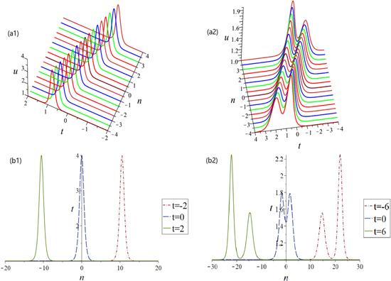
Figure 1. (a1) Bell-shaped one-soliton structure with parameters λ1 = 4, λ2 = 2, r1 = − r2 = 1; (b1) The propagation processes for one-soliton solution at t = −2 (dashdot line), t = 0 (longdash line) and t = 2 (solid line). (a2) Bell-shaped two-soliton structure with parameters ${\lambda }_{1}=\tfrac{5}{2},{\lambda }_{2}=3,{r}_{1}=-{r}_{2}=-1$; (b2) The propagation processes for two-soliton solution at t = −6 (dashdot line), t = 0 (longdash line) and t = 6 (solid line). |
| I | (I)If one of the parameters λ1 and λ2 is equal to 2, without losing generality, let λ2 = 2, we can get the one-soliton solution by the expression ( $\begin{eqnarray}{\tilde{u}}_{n}=1+\displaystyle \frac{{\lambda }_{1}^{2}-4}{4}{{\rm{sech}} }^{2}\xi ,\end{eqnarray}$ with $\begin{eqnarray*}\xi =n\mathrm{ln}\left(\displaystyle \frac{{\lambda }_{1}}{2}+\displaystyle \frac{\sqrt{{\lambda }_{1}^{2}-4}}{2}\right)+\displaystyle \frac{{\lambda }_{1}\sqrt{{\lambda }_{1}^{2}-4}}{2}t,\end{eqnarray*}$ where ∣λ1∣ > 2. From (In order to analyze the propagation stability of the one-soliton solution, we numerically simulate it by using the finite difference method [34], which is given by figure 2. Figure 2(a) shows the exact one-soliton solution, which is consistent with figure 1(a1). Figure 2(b) is the numerical solution without any noise, which is almost the same as the exact solution in figure 2(a). Figure 2(c) is the time evolution of the numerical solution after increasing a 2% noise to an exact solution. We can find that it has little change compared with the numerical solution in figure 2(b). When we increase a 5% noise, the numerical solution will change more obviously, but its overall shape will not change greatly, as is shown in figure 2(d). The numerical simulation result further illustrates the correctness of the one-soliton solution, and the soliton propagation resists small noise and keeps stability in a relatively short time. |
| II | (II)If neither λ1 nor λ2 are equal to 2, we can derive the two-soliton solution from ( $\begin{eqnarray}{\tilde{u}}_{n}=1-\displaystyle \frac{2({\lambda }_{1}^{2}-{\lambda }_{2}^{2})[({\lambda }_{2}^{2}-4)\cosh (2{\xi }_{1})+({\lambda }_{1}^{2}-4)\cosh (2{\xi }_{2})-{\lambda }_{1}^{2}+{\lambda }_{2}^{2}]}{{\left[({\lambda }_{1}\sqrt{{\lambda }_{2}^{2}-4}-{\lambda }_{2}\sqrt{{\lambda }_{1}^{2}-4})\cosh ({\xi }_{1}+{\xi }_{2})+({\lambda }_{1}\sqrt{{\lambda }_{2}^{2}-4}+{\lambda }_{2}\sqrt{{\lambda }_{1}^{2}-4})\cosh ({\xi }_{1}-{\xi }_{2})\right]}^{2}},\end{eqnarray}$ where ${\xi }_{i}=n\mathrm{ln}$ $\left(\tfrac{{\lambda }_{i}}{2}+\tfrac{\sqrt{{\lambda }_{i}^{2}-4}}{2}\right)$ + $\tfrac{{\lambda }_{i}\sqrt{{\lambda }_{i}^{2}-4}}{2}t$, ∣λi∣ > 2 (i = 1, 2). Using the asymptotic analysis technique (see [30–33] and references therein), we can give the following four kinds of asymptotic states of two-soliton solution ( |
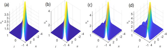
Figure 2. One-soliton solution ( |
Table 1. Physical characteristics of one-soliton solution. |
| Soliton | Amplitude | Width | Velocity | Wave number | Primary phase | Energy |
|---|---|---|---|---|---|---|
| un | $\tfrac{{\lambda}_{1}^{2}}{4}$ | $\tfrac{1}{\mathrm{ln}\left(\tfrac{{\lambda}_{1}}{2}+\tfrac{\sqrt{{\lambda}_{1}^{2}-4}}{2}\right)}$ | $-\tfrac{{\lambda}_{1}\sqrt{{\lambda}_{1}^{2}-4}}{2\mathrm{ln}\left(\tfrac{{\lambda}_{1}}{2}+\tfrac{\sqrt{{\lambda}_{1}^{2}-4}}{2}\right)}$ | $\mathrm{ln}\left(\tfrac{{\lambda}_{1}}{2}+\tfrac{\sqrt{{\lambda}_{1}^{2}-4}}{2}\right)$ | 0 | $\tfrac{{\left({\lambda}_{1}^{2}-4\right)}^{2}}{12\mathrm{ln}\left(\tfrac{{\lambda}_{1}}{2}+\tfrac{\sqrt{{\lambda}_{1}^{2}-4}}{2}\right)}$ |
Table 2. Physical characteristics of the two-soliton solution. |
| Solitons | Amplitudes | Widths | Velocities | Wave numbers | Primary phases | Energies |
|---|---|---|---|---|---|---|
| ${u}_{1}^{-}$ | $\tfrac{{\lambda}_{1}^{2}}{4}$ | $\tfrac{1}{\mathrm{ln}\left(\tfrac{{\lambda}_{1}}{2}+\tfrac{\sqrt{{\lambda}_{1}^{2}-4}}{2}\right)}$ | $-\tfrac{{\lambda}_{1}\sqrt{{\lambda}_{1}^{2}-4}}{2\mathrm{ln}\left(\tfrac{{\lambda}_{1}}{2}+\tfrac{\sqrt{{\lambda}_{1}^{2}-4}}{2}\right)}$ | $\mathrm{ln}\left(\tfrac{{\lambda}_{1}}{2}+\tfrac{\sqrt{{\lambda}_{1}^{2}-4}}{2}\right)$ | $-\tfrac{1}{2}\mathrm{ln}\tfrac{{\left({\lambda}_{1}\sqrt{{\lambda}_{2}^{2}-4}-{\lambda}_{2}\sqrt{{\lambda}_{1}^{2}-4}\right)}^{2}}{4({\lambda}_{2}^{2}-{\lambda}_{1}^{2})}$ | $\tfrac{{\left({\lambda}_{1}^{2}-4\right)}^{2}}{12\mathrm{ln}\left(\tfrac{{\lambda}_{1}}{2}+\tfrac{\sqrt{{\lambda}_{1}^{2}-4}}{2}\right)}$ |
| ${u}_{2}^{-}$ | $\tfrac{{\lambda}_{2}^{2}}{4}$ | $\tfrac{1}{\mathrm{ln}\left(\tfrac{{\lambda}_{2}}{2}+\tfrac{\sqrt{{\lambda}_{2}^{2}-4}}{2}\right)}$ | $-\tfrac{{\lambda}_{2}\sqrt{{\lambda}_{2}^{2}-4}}{2\mathrm{ln}\left(\tfrac{{\lambda}_{2}}{2}+\tfrac{\sqrt{{\lambda}_{2}^{2}-4}}{2}\right)}$ | $\mathrm{ln}\left(\tfrac{{\lambda}_{2}}{2}+\tfrac{\sqrt{{\lambda}_{2}^{2}-4}}{2}\right)$ | $-\tfrac{1}{2}\mathrm{ln}\tfrac{{\left({\lambda}_{1}\sqrt{{\lambda}_{2}^{2}-4}-{\lambda}_{2}\sqrt{{\lambda}_{1}^{2}-4}\right)}^{2}}{4({\lambda}_{2}^{2}-{\lambda}_{1}^{2})}$ | $\tfrac{{\left({\lambda}_{2}^{2}-4\right)}^{2}}{12\mathrm{ln}\left(\tfrac{{\lambda}_{2}}{2}+\tfrac{\sqrt{{\lambda}_{2}^{2}-4}}{2}\right)}$ |
| ${u}_{1}^{+}$ | $\tfrac{{\lambda}_{1}^{2}}{4}$ | $\tfrac{1}{\mathrm{ln}\left(\tfrac{{\lambda}_{1}}{2}+\tfrac{\sqrt{{\lambda}_{1}^{2}-4}}{2}\right)}$ | $-\tfrac{{\lambda}_{1}\sqrt{{\lambda}_{1}^{2}-4}}{2\mathrm{ln}\left(\tfrac{{\lambda}_{1}}{2}+\tfrac{\sqrt{{\lambda}_{1}^{2}-4}}{2}\right)}$ | $\mathrm{ln}\left(\tfrac{{\lambda}_{1}}{2}+\tfrac{\sqrt{{\lambda}_{1}^{2}-4}}{2}\right)$ | $\tfrac{1}{2}\mathrm{ln}\tfrac{{\left({\lambda}_{1}\sqrt{{\lambda}_{2}^{2}-4}-{\lambda}_{2}\sqrt{{\lambda}_{1}^{2}-4}\right)}^{2}}{4({\lambda}_{2}^{2}-{\lambda}_{1}^{2})}$ | $\tfrac{{\left({\lambda}_{1}^{2}-4\right)}^{2}}{12\mathrm{ln}\left(\tfrac{{\lambda}_{1}}{2}+\tfrac{\sqrt{{\lambda}_{1}^{2}-4}}{2}\right)}$ |
| ${u}_{2}^{+}$ | $\tfrac{{\lambda}_{2}^{2}}{4}$ | $\tfrac{1}{\mathrm{ln}\left(\tfrac{{\lambda}_{2}}{2}+\tfrac{\sqrt{{\lambda}_{2}^{2}-4}}{2}\right)}$ | $-\tfrac{{\lambda}_{2}\sqrt{{\lambda}_{2}^{2}-4}}{2\mathrm{ln}\left(\tfrac{{\lambda}_{2}}{2}+\tfrac{\sqrt{{\lambda}_{2}^{2}-4}}{2}\right)}$ | $\mathrm{ln}\left(\tfrac{{\lambda}_{2}}{2}+\tfrac{\sqrt{{\lambda}_{2}^{2}-4}}{2}\right)$ | $\tfrac{1}{2}\mathrm{ln}\tfrac{{\left({\lambda}_{1}\sqrt{{\lambda}_{2}^{2}-4}-{\lambda}_{2}\sqrt{{\lambda}_{1}^{2}-4}\right)}^{2}}{4({\lambda}_{2}^{2}-{\lambda}_{1}^{2})}$ | $\tfrac{{\left({\lambda}_{2}^{2}-4\right)}^{2}}{12\mathrm{ln}\left(\tfrac{{\lambda}_{2}}{2}+\tfrac{\sqrt{{\lambda}_{2}^{2}-4}}{2}\right)}$ |
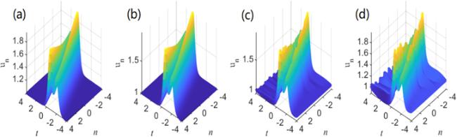
Figure 3. Two-soliton solution ( |
5.2. Rational solutions and asymptotic analysis
| I | (I)When N = 1, we can get the first-order rational solution by the generalized (1, 1)-fold DT as follows: $\begin{eqnarray}{\tilde{u}}_{n}={d}_{n+1}^{(2)}{u}_{n}+{c}_{n+1}^{(1)},\end{eqnarray}$ where ${a}_{n}^{(0)}=\tfrac{{\rm{\Delta }}{a}_{n}^{(0)}}{{{\rm{\Delta }}}_{1}}$, ${c}_{n}^{(1)}={a}_{n}^{(0)}\tfrac{{\rm{\Delta }}{c}_{n}^{(1)}}{{{\rm{\Delta }}}_{2}}$ and ${d}_{n}^{(2)}={a}_{n}^{(0)}\tfrac{{\rm{\Delta }}{d}_{n}^{(2)}}{{{\rm{\Delta }}}_{2}}$, in which $\begin{eqnarray*}\begin{array}{l}{{\rm{\Delta }}}_{1}=\left|\begin{array}{cc}{\varphi }_{n}^{(0)} & {\lambda }_{1}{\psi }_{n}^{(0)}\\ {\varphi }_{n}^{(1)} & {\lambda }_{1}{\psi }_{n}^{(1)}+{\psi }_{n}^{(0)}\end{array}\right|,\\ {{\rm{\Delta }}}_{2}=\left|\begin{array}{cc}{\lambda }_{1}{\varphi }_{n}^{(0)} & {\lambda }_{1}^{2}{\psi }_{n}^{(0)}\\ {\lambda }_{1}{\varphi }_{n}^{(1)}+{\varphi }_{n}^{(0)} & {\lambda }_{1}^{2}{\psi }_{n}^{(1)}+2{\lambda }_{1}{\psi }_{n}^{(0)}\end{array}\right|,\\ {\rm{\Delta }}{c}_{n}^{(1)}=\left|\begin{array}{cc}-{\psi }_{n}^{(0)} & {\lambda }_{1}^{2}{\psi }_{n}^{(0)}\\ -{\psi }_{n}^{(1)} & {\lambda }_{1}^{2}{\psi }_{n}^{(1)}+2{\lambda }_{1}{\psi }_{n}^{(0)}\end{array}\right|,\\ {\rm{\Delta }}{a}_{n}^{(0)}=\left|\begin{array}{cc}-{\lambda }_{1}^{2}{\varphi }_{n}^{(0)} & {\lambda }_{1}{\psi }_{n}^{(0)}\\ -{\lambda }_{1}^{2}{\varphi }_{n}^{(1)}-2{\lambda }_{1}{\varphi }_{n}^{(0)} & {\lambda }_{1}{\psi }_{n}^{(1)}+{\psi }_{n}^{(0)}\end{array}\right|,\\ {\rm{\Delta }}{d}_{n}^{(2)}=\left|\begin{array}{cc}{\lambda }_{1}{\varphi }_{n}^{(0)} & -{\psi }_{n}^{(0)}\\ {\lambda }_{1}{\varphi }_{n}^{(1)}+{\varphi }_{n}^{(0)} & -{\psi }_{n}^{(1)}\end{array}\right|,\end{array}\end{eqnarray*}$ where ${a}_{n+1}^{(0)}$, ${c}_{n+1}^{(1)}$ and ${d}_{n+1}^{(2)}$ are obtained from ${a}_{n}^{(0)}$, ${c}_{n}^{(1)}$ and ${d}_{n}^{(2)}$ by changing n into n + 1. From the above formulas, we can calculate the expression of equation ( $\begin{eqnarray}{\tilde{u}}_{n}=1-\displaystyle \frac{1}{{\left(n+2t+2{e}_{0}\right)}^{2}}=1-\displaystyle \frac{1}{{\left(\xi +2{e}_{0}\right)}^{2}},\end{eqnarray}$ from which we can see that solution ( |
| II | (II)When N = 2, we can get the second-order rational solution by the generalized (1, 3)-fold DT as $\begin{eqnarray}{\tilde{u}}_{n}={d}_{n+1}^{(4)}{u}_{n}+{c}_{n+1}^{(3)},\end{eqnarray}$ where ${a}_{n}^{(0)}=\tfrac{{\rm{\Delta }}{a}_{n}^{(0)}}{{{\rm{\Delta }}}_{1}}$, ${c}_{n}^{(3)}={a}_{n}^{(0)}\tfrac{{\rm{\Delta }}{c}_{n}^{(3)}}{{{\rm{\Delta }}}_{2}}$ and ${d}_{n}^{(4)}={a}_{n}^{(0)}\tfrac{{\rm{\Delta }}{d}_{n}^{(4)}}{{{\rm{\Delta }}}_{2}}$, in which |
| i | (i)If ${\zeta }_{1}=n+2t-{\left(10+6\sqrt{5}\right)}^{\tfrac{1}{3}}{t}^{\tfrac{1}{3}}$ is regarded as a fixed constant, we can obtain ${\zeta }_{2}={\zeta }_{1}+{{bt}}^{\tfrac{1}{3}}$ and ζ2 → ± ∞ when t → ± ∞ , from which we can get that the first two limit states are $\begin{eqnarray}{\tilde{u}}_{n}\to {u}_{1}^{\pm }=1-\displaystyle \frac{1}{{\left({\zeta }_{1}+2{e}_{0}\right)}^{2}}.\end{eqnarray}$ |
| ii | (ii)If ${\zeta }_{2}=n+2t-{\left(10-6\sqrt{5}\right)}^{\tfrac{1}{3}}{t}^{\tfrac{1}{3}}$ is regarded as a fixed constant, we can obtain ${\zeta }_{1}={\zeta }_{2}-{{bt}}^{\tfrac{1}{3}}$ and ζ1 → ∓ ∞ when t → ± ∞ , from which we can get that the last two limit states are $\begin{eqnarray}{\tilde{u}}_{n}\to {u}_{2}^{\pm }=1-\displaystyle \frac{1}{{\left({\zeta }_{2}+2{e}_{0}\right)}^{2}}.\end{eqnarray}$ |
Table 3. Main mathematical features of rational solution ${\tilde{u}}_{n}$ of order N. |
| N | Background of ${\tilde{u}}_{n}$ | Highest powers in the numerator | Highest powers in the denominator |
|---|---|---|---|
| 1 | 1 | 2 | 2 |
| 2 | 1 | 12 | 12 |
| 3 | 1 | 30 | 30 |
| ... | ... | ... | ... |
| N | 1 | 2N(2N − 1) | 2N(2N − 1) |
It should be noted here that for discrete KdV equation (
5.3. Mixed solution and asymptotic state analysis
| i | (i)If ξ1 is equal to a fixed constant as t → ± ∞ , we can get ξ2 → ± ∞ , and two asymptotic states of solution ( $\begin{eqnarray}{\tilde{u}}_{n}\to {u}_{1}^{\pm }=1-3{\mathrm{csch}}^{2}{\xi }_{1},\end{eqnarray}$ where ${u}_{1}^{-},{u}_{1}^{+}$ stand for the limit states of solution ( |
| ii | (ii)If ξ2 is equal to a fixed constant as t → ± ∞ , we can get ξ1 → ± ∞ , and two asymptotic states of solution ( |
It should be noted here that for this case, we should get mixed superposition solutions of usual soliton and rational solution in theory. However, from the above analysis, we know that when ${\xi }_{1}$ is fixed and ${\xi }_{2}\to \pm \infty $, the asymptotic states of the mixed solution (