


1. Introduction
It is well known that a spin-1/2 state (or a two-level state) can be described by a point in the sphere, which is called the Bloch representation. Quantum dynamics of the spin-1/2 system can be studied geometrically via the trajectory of a point in the Bloch sphere. Extension of this representation to a higher dimensional quantum state has been brilliantly resolved by Majorana [1]. The main spirit is to represent a generic spin-J state (equivalent to n body two-mode boson state with n = 2J or a symmetric n qubit state) by 2J points in a two-dimensional Majorana sphere rather than a higher dimensional sphere. Then the evolution of the generic spin-J state can be intuitively described by 2J points in the Majorana sphere [2], in which the 2J points are called Majorana stars. The Majorana's stellar representation (MSR) has attracted much attention in various fields [3–6], such as the many-body phenomenon [5, 7, 8], spinor Bose–Einstein condensation [4, 9], non-Hermitian multiband systems [10, 11], geometric phases [12–15] and different physical models [16–19].
Now we introduce the Majorana stellar representation. Majorana has given a wonderful relation between the generic spin-J state and n = 2J points in the Majorana sphere, so a generic spin-J state can also be represented by [1, 13, 14]2 ). Then the 2J points have been found and that is the so-called Majorana stellar representation.
$\begin{eqnarray}\begin{array}{rcl}| \psi \rangle & = & \sum _{m=-J}^{J}{C}_{m}| J,m\rangle \\ & = & \displaystyle \frac{1}{\sqrt{n!}{N}_{n}}\sum _{P}| {u}_{P(1)}\rangle \otimes | {u}_{P(2)}\rangle \otimes \cdots | {u}_{P(n)}\rangle ,\end{array}\end{eqnarray}$
where P means the sum of all permutations of the 2J points. Here, ∣uk⟩ is a spin-1/2 state, and the corresponding θk and φk are determined by the following procedure. In the Schwinger representation, a spin-J state induces a star equation [13]: $\begin{eqnarray}\sum _{k=0}^{2J}\displaystyle \frac{{(-1)}^{2J-k}{C}_{k-J}}{\sqrt{(2J-k)!k!}}{z}^{k}=0,\end{eqnarray}$
where ${z}_{k}=\tan \tfrac{{\theta }_{k}}{2}{{\rm{e}}}^{{\rm{i}}{\phi }_{k}}$ is one of the 2J roots of the equation (The quantum geometric tensor (QGT), comprising the Berry curvature and the quantum metric tensor, exhibits the geometric property of a quantum state. It has played an indispensable role in many frontier topics of quantum information and condensed matter physics [11, 20–24]. The gauge-invariant QGT was first proposed by Provost and Vallee in 1980 [25]. Its real part is in the form of the quantum metric tensor, whereas its imaginary part corresponds to the Berry curvature [26, 27]. Both the real and imaginary parts have been discussed in various contexts. For example, the Berry curvature, which emerges during a cyclic evolution, has contributed to the correction of Bloch electron group velocity [28, 29] and the dynamical quantum Hall effect in the parameter space [30]. As for the quantum metric tensor, not only does it play a central role in the quantum metrology known as Fisher information [31, 32], but also manifests the superfluid's stiffness with respect to magnetic gradients in the hydrodynamics of spinor condensates [4].
The gauge-invariant quantity, QGT, can be written as [25]
$\begin{eqnarray}{Q}_{\alpha \beta }=\langle {\partial }_{\alpha }\chi | {\partial }_{\beta }\chi \rangle -\langle {\partial }_{\alpha }\chi | \chi \rangle \langle \chi | {\partial }_{\beta }\chi \rangle ,\end{eqnarray}$
where ∣χ⟩ is a normalized state, and α and β are two parameters in the parameter space of the Hamiltonian. It is easy to show the real part of the QGT is its symmetric part, which is a quarter of the quantum Fisher information matrix [21] $\begin{eqnarray}{g}_{\alpha \beta }\equiv \mathrm{Re}[{Q}_{\alpha \beta }]=\displaystyle \frac{1}{4}{F}_{\alpha \beta },\end{eqnarray}$
where the Fαβ is the well-known quantum Fisher information matrix. As for the imaginary part of the QGT, it is the antisymmetric part and is equivalent to the Berry curvature except for a constant coefficient [22, 23] $\begin{eqnarray}\mathrm{Im}[{Q}_{\alpha \beta }]=-\displaystyle \frac{1}{2}\left[{\rm{i}}\left(\langle {\partial }_{\alpha }\chi | {\partial }_{\beta }\chi \rangle -\langle {\partial }_{\beta }\chi | {\partial }_{\alpha }\chi \rangle \right)\right].\end{eqnarray}$
The expression in the square bracket in the last equation is exactly the Berry curvature. As a result, the quantum geometric tensor combines two extremely important geometric quantities in one expression.In the past decades, there have been lots of advances in the representation of the Berry phase using the MSR. The individual motions of the Majorana stars and the correlations between stars have been thought to be linked with the Berry phase and quantum entanglement [13, 14, 33]. As for the quantum metric tensor, its diagonal elements have been identified with the CPN model for a general spin J = n/2 [4], and it also reveals some intrinsic relations with quantum phase transition [21, 22, 34–36]. However, the direct representation of the QGT by the MSR has not been studied.
In this article, we will use the spherical coordinates to obtain the relations between the quantum state and the Bloch vector. Using these relations, we further derive the MSR of QGT up to spin-3/2 situation. Our method is essentially identified with that of the [4], and the real and imaginary parts of our results are the same with those respectively.
This article is organized as follows. In section 2 , we introduce the spherical coordinates representation of an arbitrary two-level state. Furthermore, we get a set of relations between the two-level state and the Bloch vector and give the simple expression of the QGT using MSR with respect to spin-1/2 and spin-1 situations. In section 3 , we derive the QGT of the spin-3/2 and discuss two simple cases to demonstrate the MSR for QGT. In section 4 , we use a simple Lipkin–Meshkov–Glick (LMG) model to verify the correctness of the results in section 3 . In section 5 , the results of special situations of the arbitrary spin state are given. A brief conclusion is given in section 6 .
2. Spherical coordinate representation of one or two-qubit and its application
As a well-known fact, a general spin-1/2 pure state can be described as:13 ) is actually the diagonal element of the quantum metric tensor for spin-1/2 states. And there are three useful equations in the calculation of QGT:
$\begin{eqnarray}| u\rangle =\cos \displaystyle \frac{\theta }{2}{{\rm{e}}}^{-{\rm{i}}\tfrac{\phi }{2}}| \uparrow \rangle +\sin \displaystyle \frac{\theta }{2}{{\rm{e}}}^{{\rm{i}}\tfrac{\phi }{2}}| \downarrow \rangle ,\end{eqnarray}$
and then the pure state ∣u⟩ can be represented as (θ, φ) in the Bloch sphere. We next define a state orthogonal to ∣u⟩: $\begin{eqnarray}| {u}^{\perp }\rangle =-\sin \displaystyle \frac{\theta }{2}{{\rm{e}}}^{-{\rm{i}}\tfrac{\phi }{2}}| \uparrow \rangle +\cos \displaystyle \frac{\theta }{2}{{\rm{e}}}^{{\rm{i}}\tfrac{\phi }{2}}| \downarrow \rangle ,\end{eqnarray}$
where a global phase factor has been ignored and it corresponds to a point (π − θ, π + φ) in the Bloch sphere. Then the state ∣u⟩ can be represented as $\vec{n}=(\sin \theta \cos \phi ,\sin \theta \sin \phi ,\cos \theta )$ in the spherical coordinate representation, whereas the orthogonal state ∣u⊥⟩ corresponds to $-\vec{n}$. We further introduce two mutually orthogonal vectors which are also perpendicular to the Bloch vector $\vec{n}$: ${\vec{n}}_{x}=(\cos \theta \cos \phi ,\cos \theta \sin \phi ,-\sin \theta )$, ${\vec{n}}_{y}=(-\sin \phi ,\cos \phi ,0)$, and the $({\vec{n}}_{x},{\vec{n}}_{y},\vec{n})$ constitutes right-handed Cartesian coordinate system. Furthermore, we define two vectors analogous to the creation and annihilation operators: ${\vec{n}}_{+}={\vec{n}}_{x}+{\rm{i}}{\vec{n}}_{y}$, ${\vec{n}}_{-}={\vec{n}}_{x}-{\rm{i}}{\vec{n}}_{y}$. It is easy to show $\begin{eqnarray}\begin{array}{rcl}{\vec{n}}_{-}{\vec{n}}_{+}\cdot {\partial }_{\alpha }\vec{n} & = & {\partial }_{\alpha }\vec{n}-{\rm{i}}\vec{n}\times {\partial }_{\alpha }\vec{n},\\ {\vec{n}}_{+}{\vec{n}}_{-}\cdot {\partial }_{\alpha }\vec{n} & = & {\partial }_{\alpha }\vec{n}+{\rm{i}}\vec{n}\times {\partial }_{\alpha }\vec{n},\end{array}\end{eqnarray}$
where α is an arbitrary parameter. Given the above definitions, we have $\begin{eqnarray}\begin{array}{rcl}{\partial }_{\alpha }\vec{n} & = & {\partial }_{\alpha }\theta {\vec{n}}_{x}+\sin \theta {\partial }_{\alpha }\phi {\vec{n}}_{y},\\ {\partial }_{\alpha }{\vec{n}}_{x} & = & -{\partial }_{\alpha }\theta \vec{n}+\cos \theta {\partial }_{\alpha }\phi {\vec{n}}_{y},\\ {\partial }_{\alpha }{\vec{n}}_{y} & = & -{\partial }_{\alpha }\phi (\sin \theta \vec{n}+\cos \theta {\vec{n}}_{x}).\end{array}\end{eqnarray}$
Since we have the above properties, the relation between a pure state and the Bloch vector can be more clear now: $\begin{eqnarray}\begin{array}{rcl}\langle u| \vec{\sigma }| u\rangle & = & \vec{n},\\ \langle {u}^{\perp }| \vec{\sigma }| {u}^{\perp }\rangle & = & -\vec{n},\\ \langle u| \vec{\sigma }| {u}^{\perp }\rangle & = & {\vec{n}}_{-},\\ \langle {u}^{\perp }| \vec{\sigma }| u\rangle & = & {\vec{n}}_{+}.\end{array}\end{eqnarray}$
The Berry connection for the 1-qubit pure state becomes $\begin{eqnarray}{\rm{i}}\langle u| {\partial }_{\alpha }u\rangle =\displaystyle \frac{1}{2}\cos \theta {\partial }_{\alpha }\phi =\displaystyle \frac{1}{2}{\vec{n}}_{y}\cdot {\partial }_{\alpha }{\vec{n}}_{x}\equiv {a}_{\alpha }.\end{eqnarray}$
In addition, using those properties, we can get: $\begin{eqnarray}\langle {u}^{\perp }| {\partial }_{\alpha }u\rangle =\displaystyle \frac{1}{2}{\partial }_{\alpha }\theta +\displaystyle \frac{{\rm{i}}}{2}\sin \theta {\partial }_{\alpha }\phi =\displaystyle \frac{1}{2}{\vec{n}}_{+}\cdot {\partial }_{\alpha }\vec{n},\end{eqnarray}$
$\begin{eqnarray}{F}_{\alpha }\equiv \langle {\partial }_{\alpha }u| {u}^{\perp }\rangle \langle {u}^{\perp }| {\partial }_{\alpha }u\rangle =\displaystyle \frac{1}{4}{\partial }_{\alpha }\vec{n}\cdot {\partial }_{\alpha }\vec{n}.\end{eqnarray}$
The equation ( $\begin{eqnarray}\langle {\partial }_{\alpha }u| {\partial }_{\alpha }u\rangle ={a}_{\alpha }^{2}+{F}_{\alpha },\end{eqnarray}$
$\begin{eqnarray}\langle u| \vec{\sigma }| {\partial }_{\alpha }u\rangle =\displaystyle \frac{1}{2}{\partial }_{\alpha }\vec{n}+\displaystyle \frac{{\rm{i}}}{2}{\partial }_{\alpha }\vec{n}\times \vec{n}-{\rm{i}}{a}_{\alpha }\vec{n},\end{eqnarray}$
$\begin{eqnarray}\langle {u}^{\perp }| \vec{\sigma }| {\partial }_{\alpha }u\rangle =-{\rm{i}}{a}_{\alpha }{\vec{n}}_{+}-\displaystyle \frac{1}{2}{\vec{n}}_{+}\cdot {\partial }_{\alpha }\vec{n}\ \vec{n}.\end{eqnarray}$
We are now in a position to start the calculation of the MSR for QGT. For an unnormalized state $| \vec{u}\rangle \,$ ≡$\,\tfrac{1}{\sqrt{N!}}$ ∑P∣uP(1)⟩ ⨂ ∣uP(2)⟩ ⨂ ⋯ ∣uP(N)⟩, the corresponding normalized state is $| \chi \rangle =\tfrac{| \vec{u}\rangle }{\sqrt{\langle \vec{u}| \vec{u}\rangle }}$. And the QGT for this case becomes [8]
$\begin{eqnarray}\begin{array}{rcl}{Q}_{\alpha \beta } & = & \langle {\partial }_{\alpha }\chi | {\partial }_{\beta }\chi \rangle -\langle {\partial }_{\alpha }\chi | \chi \rangle \langle \chi | {\partial }_{\beta }\chi \rangle \\ & = & \displaystyle \frac{\langle {\partial }_{\alpha }\vec{u}| {\partial }_{\beta }\vec{u}\rangle \langle \vec{u}| \vec{u}\rangle -\langle {\partial }_{\alpha }\vec{u}| \vec{u}\rangle \langle \vec{u}| {\partial }_{\beta }\vec{u}\rangle }{\langle \vec{u}| \vec{u}{\rangle }^{2}}.\end{array}\end{eqnarray}$
We will begin from the simplest case with spin-1/2. In this situation, we can let $| \chi \rangle =| \vec{u}\rangle =| u\rangle $. The state has been normalized for the case of spin-1/2. Then we obtain the QGT
$\begin{eqnarray}\begin{array}{rcl}{Q}_{\alpha \beta } & = & \langle {\partial }_{\alpha }\chi | {\partial }_{\beta }\chi \rangle -\langle {\partial }_{\alpha }\chi | \chi \rangle \langle \chi | {\partial }_{\beta }\chi \rangle \\ & = & \langle {\partial }_{\alpha }u| {u}^{\perp }\rangle \langle {u}^{\perp }| {\partial }_{\beta }u\rangle \\ & = & \displaystyle \frac{1}{4}\left[{\partial }_{\alpha }\vec{n}\cdot {\partial }_{\beta }\vec{n}+{\rm{i}}\vec{n}\cdot \left({\partial }_{\alpha }\vec{n}\times {\partial }_{\beta }\vec{n}\right)\right].\end{array}\end{eqnarray}$
The real and imaginary part gives the quantum metric and Berry curvature respectively.When it comes to spin-1 situation, a generic spin-1 pure state can be written as the permutation form:
$\begin{eqnarray}| \chi \rangle =\displaystyle \frac{1}{{{ \mathcal N }}_{2}}| \vec{u}\rangle =\displaystyle \frac{1}{{{ \mathcal N }}_{2}\sqrt{2}}\left(| {u}_{1}\rangle \otimes | {u}_{2}\rangle +| {u}_{2}\rangle \otimes | {u}_{1}\rangle \right),\end{eqnarray}$
where the normalization coefficient [8, 14] is $\begin{eqnarray}{{ \mathcal N }}_{2}^{2}=\langle \vec{u}| \vec{u}\rangle =\displaystyle \frac{3+{\vec{n}}_{1}\cdot {\vec{n}}_{2}}{2}.\end{eqnarray}$
In order to get the QGT, we need to calculate several terms utilizing the relations above: $\begin{eqnarray}\begin{array}{rcl}\langle {\partial }_{\alpha }\vec{u}| {\partial }_{\beta }\vec{u}\rangle & = & \left[\langle {\partial }_{\alpha }{u}_{1}| {\partial }_{\beta }{u}_{1}\rangle +\langle {u}_{1}| {\partial }_{\beta }{u}_{1}\rangle \langle {\partial }_{\alpha }{u}_{2}| {u}_{2}\rangle \right.\\ & & \left.+\langle {\partial }_{\alpha }{u}_{1}| {\partial }_{\beta }{u}_{2}\rangle \langle {u}_{2}| {u}_{1}\rangle +\langle {u}_{1}| {\partial }_{\beta }{u}_{2}\rangle \langle {\partial }_{\alpha }{u}_{2}| {u}_{1}\rangle \right]\\ & & +\left[1\leftrightarrow 2\right].\end{array}\end{eqnarray}$
The last line in equation (21 ) is nothing but swapping the subscripts 1 and 2 in the above four terms So we just need to calculate the first two lines. Besides, we still need to calculate the two-star Berry connection
$\begin{eqnarray}\langle \vec{u}| {\partial }_{\alpha }\vec{u}\rangle =\left[\langle {u}_{1}| {\partial }_{\alpha }{u}_{1}\rangle +\langle {u}_{1}| {u}_{2}\rangle \langle {u}_{2}| {\partial }_{\alpha }{u}_{1}\rangle \right]+\left[1\leftrightarrow 2\right].\end{eqnarray}$
After calculating these terms using the equations in section 2 , we can obtain the explicit form of QGT represented by Bloch vectors. Since the full expression of the QGT is not so brief, we just give its real and imaginary parts individually. The real part of the QGT can be simplified as
$\begin{eqnarray}\begin{array}{rcl}\mathrm{Re}{Q}_{\alpha \beta } & = & \displaystyle \frac{4}{{(3+{\vec{n}}_{1}\cdot {\vec{n}}_{2})}^{2}}\left(\displaystyle \frac{1}{2}{\partial }_{\alpha }{\vec{n}}_{1}\cdot {\partial }_{\beta }{\vec{n}}_{1}+\displaystyle \frac{1}{2}{\partial }_{\alpha }{\vec{n}}_{2}\cdot {\partial }_{\beta }{\vec{n}}_{2}\right.\\ & & +\displaystyle \frac{1+{\vec{n}}_{1}\cdot {\vec{n}}_{2}}{4}{\partial }_{\alpha }{\vec{n}}_{1}\cdot {\partial }_{\beta }{\vec{n}}_{2}+\displaystyle \frac{1+{\vec{n}}_{1}\cdot {\vec{n}}_{2}}{4}{\partial }_{\alpha }{\vec{n}}_{2}\cdot {\partial }_{\beta }{\vec{n}}_{1}\\ & & \left.-\displaystyle \frac{1}{4}{\vec{n}}_{2}\cdot {\partial }_{\alpha }{\vec{n}}_{1}\ {\vec{n}}_{1}\cdot {\partial }_{\beta }{\vec{n}}_{2}-\displaystyle \frac{1}{4}{\vec{n}}_{1}\cdot {\partial }_{\alpha }{\vec{n}}_{2}\ {\vec{n}}_{2}\cdot {\partial }_{\beta }{\vec{n}}_{1}\right),\end{array}\end{eqnarray}$
and the imaginary part of the QGT is $\begin{eqnarray}\begin{array}{rcl}\mathrm{Im}{Q}_{\alpha \beta } & = & \displaystyle \frac{4}{{(3+{\vec{n}}_{1}\cdot {\vec{n}}_{2})}^{2}}\left\{\displaystyle \frac{1}{2}{\vec{n}}_{1}\cdot \left({\partial }_{\alpha }{\vec{n}}_{1}\times {\partial }_{\beta }{\vec{n}}_{1}\right)\right.\\ & & +\displaystyle \frac{1}{2}{\vec{n}}_{2}\cdot \left({\partial }_{\alpha }{\vec{n}}_{2}\times {\partial }_{\beta }{\vec{n}}_{2}\right)+\displaystyle \frac{1}{4}{\partial }_{\alpha }{\vec{n}}_{1}\times {\partial }_{\beta }{\vec{n}}_{2}\cdot \left({\vec{n}}_{1}+{\vec{n}}_{2}\right)\\ & & \left.+\displaystyle \frac{1}{4}{\partial }_{\alpha }{\vec{n}}_{2}\times {\partial }_{\beta }{\vec{n}}_{1}\cdot \left({\vec{n}}_{1}+{\vec{n}}_{2}\right)\right\}.\end{array}\end{eqnarray}$
This result is identified with that of the [4], whereas we obtain it from the expression of QGT rather than the direct calculation of the Berry curvature and the quantum metric tensor.
The situation in the spin-1 is still clear. The quantum geometric tensor includes the contribution not only from each Majorana stars but from the interaction between them. The case in spin-3/2 is basically the same, but the interaction part is more complex.
3. MSR of the QGT for three-qubit case
3.1. Calculation for the three-qubit case
Following the same procedure, a generic spin-3/2 pure state is27 ). This term can be explicitly written as
$\begin{eqnarray}\begin{array}{rcl}| \chi \rangle & = & \displaystyle \frac{1}{{{ \mathcal N }}_{3}}| \vec{u}\rangle =\displaystyle \frac{1}{{{ \mathcal N }}_{3}}\displaystyle \frac{1}{\sqrt{3!}}\left(| {u}_{1}\rangle \otimes | {u}_{2}\rangle \otimes | {u}_{3}\rangle \right.\\ & & +| {u}_{1}\rangle \otimes | {u}_{3}\rangle \otimes | {u}_{2}\rangle +| {u}_{2}\rangle \otimes | {u}_{1}\rangle \otimes | {u}_{3}\rangle \\ & & +| {u}_{2}\rangle \otimes | {u}_{3}\rangle \otimes | {u}_{1}\rangle +| {u}_{3}\rangle \otimes | {u}_{1}\rangle \otimes | {u}_{2}\rangle \\ & & \left.+| {u}_{3}\rangle \otimes | {u}_{2}\rangle \otimes | {u}_{1}\rangle \right),\end{array}\end{eqnarray}$
where now the normalization coefficient becomes $\begin{eqnarray}{{ \mathcal N }}_{3}^{2}=\langle \vec{u}| \vec{u}\rangle =3+{\vec{n}}_{1}\cdot {\vec{n}}_{2}+{\vec{n}}_{2}\cdot {\vec{n}}_{3}+{\vec{n}}_{3}\cdot {\vec{n}}_{1}.\end{eqnarray}$
Since we already have the normalization coefficient, we just need to figure out the following two expressions respectively, i.e. $\langle {\partial }_{\alpha }\vec{u}| {\partial }_{\beta }\vec{u}\rangle $ and $\langle \vec{u}| {\partial }_{\alpha }\vec{u}\rangle $. The calculation is tedious, so we only list our main results here. $\begin{eqnarray}\begin{array}{l}\langle {\partial }_{\alpha }\vec{u}| {\partial }_{\beta }\vec{u}\rangle =\sum _{P}\left(\langle {\partial }_{\alpha }{u}_{1}| \langle {u}_{2}| \langle {u}_{3}| +\langle {u}_{1}| \langle {\partial }_{\alpha }{u}_{2}| \langle {u}_{3}| \right.\\ \,\,\,\left.+\,\langle {u}_{1}| \langle {u}_{2}| \langle {\partial }_{\alpha }{u}_{3}| \right)\left(| {\partial }_{\beta }{u}_{P(1)}\rangle | {u}_{P(2)}\rangle | {u}_{P(3)}\rangle \right.\\ \,\,\,\left.+\,| {u}_{P(1)}\rangle | {\partial }_{\beta }{u}_{P(2)}\rangle | {u}_{P(3)}\rangle +| {u}_{P(1)}\rangle | {u}_{P(2)}\rangle | {\partial }_{\beta }{u}_{P(3)}\rangle \right).\end{array}\end{eqnarray}$
This term is complex but straightforward, and we need to substitute those vector formulas into the inner products of states of the equation ( $\begin{eqnarray}\begin{array}{l}\langle {\partial }_{\alpha }\vec{u}| {\partial }_{\beta }\vec{u}\rangle \\ =\,\displaystyle \frac{1}{4}({\partial }_{\alpha }{\vec{n}}_{1}+{\rm{i}}{\vec{n}}_{1}\times {\partial }_{\alpha }{\vec{n}}_{1})\cdot \left[{\partial }_{\beta }{\vec{n}}_{2}-{\rm{i}}{\vec{n}}_{2}\times {\partial }_{\beta }{\vec{n}}_{2}+{\partial }_{\beta }{\vec{n}}_{3}\right.\\ \,\,\left.-\,{\rm{i}}{\vec{n}}_{3}\times {\partial }_{\beta }{\vec{n}}_{3}+\left(3+{\vec{n}}_{2}\cdot {\vec{n}}_{3}-{\vec{n}}_{1}\cdot ({\vec{n}}_{3}+{\vec{n}}_{2})\right){\partial }_{\beta }{\vec{n}}_{1}\right]\\ \,\,+\,1\leftrightarrow 2+1\leftrightarrow 3+\mathrm{Terms}\ \mathrm{with}\,{a}_{\alpha i}\,\mathrm{and}\,{a}_{\beta i}.\end{array}\end{eqnarray}$
There are some terms concerning aαi and aβi, which do not satisfy the gauge variance. Since the QGT is gauge-invariant, this kind of term must be finally canceled.Next, we just need to calculate the term31 ). Apparently, this Berry-connection-like term is also gauge-dependent. The MSR of the second term reads28 ) and (30 ) are mutually canceled when calculating the final QGT, which stems from the gauge invariance of QGT.31 ) divided by ${{ \mathcal N }}_{3}^{4}$. We can see that the subtrahend in the last line of equation (31 ) reduces to zero when ${\vec{n}}_{1}+{\vec{n}}_{2}+{\vec{n}}_{3}\,=\,0$.
$\begin{eqnarray}\begin{array}{l}\langle \vec{u}| {\partial }_{\alpha }\vec{u}\rangle =\langle {u}_{1}| \langle {u}_{2}| \langle {u}_{3}| \sum _{P}\left(| {\partial }_{\alpha }{u}_{P(1)}\rangle | {u}_{P(2)}\rangle | {u}_{P(3)}\rangle \right.\\ \,\,\left.+\,| {u}_{P(1)}\rangle | {\partial }_{\alpha }{u}_{P(2)}\rangle | {u}_{P(3)}\rangle +| {u}_{P(1)}\rangle | {u}_{P(2)}\rangle | {\partial }_{\alpha }{u}_{P(3)}\rangle \right).\end{array}\end{eqnarray}$
Once we obtain these two terms, the concrete form of the QGT for spin-$\tfrac{3}{2}$ case can be summarized as the equation ( $\begin{eqnarray}\begin{array}{l}\langle \vec{u}| {\partial }_{\alpha }\vec{u}\rangle =\displaystyle \frac{1}{2}[{\vec{n}}_{2}+{\rm{i}}({\vec{n}}_{1}\times {\vec{n}}_{2})+{\vec{n}}_{3}+{\rm{i}}({\vec{n}}_{1}\times {\vec{n}}_{3})]\cdot {\partial }_{\alpha }{\vec{n}}_{1}\\ \,\,\,+\,\displaystyle \frac{1}{2}[{\vec{n}}_{1}+{\rm{i}}({\vec{n}}_{2}\times {\vec{n}}_{1})+{\vec{n}}_{3}+{\rm{i}}({\vec{n}}_{2}\times {\vec{n}}_{3})]\cdot {\partial }_{\alpha }{\vec{n}}_{2}\\ \,\,\,+\,\displaystyle \frac{1}{2}[{\vec{n}}_{1}+{\rm{i}}({\vec{n}}_{3}\times {\vec{n}}_{1})+{\vec{n}}_{2}+{\rm{i}}({\vec{n}}_{3}\times {\vec{n}}_{2})]\cdot {\partial }_{\alpha }{\vec{n}}_{3}\\ \,\,\,+\,\mathrm{Terms}\ \mathrm{with}\ {a}_{\alpha i}.\end{array}\end{eqnarray}$
Those gauge-variant terms in equations ( $\begin{eqnarray}\begin{array}{l}\langle {\partial }_{\alpha }\vec{u}| {\partial }_{\beta }\vec{u}\rangle \langle \vec{u}| \vec{u}\rangle -\langle {\partial }_{\alpha }\vec{u}| \vec{u}\rangle \langle \vec{u}| {\partial }_{\beta }\vec{u}\rangle \\ =\,\left[\displaystyle \frac{1}{4}({\partial }_{\alpha }{\vec{n}}_{1}+{\rm{i}}{\vec{n}}_{1}\times {\partial }_{\alpha }{\vec{n}}_{1})\cdot \left[(3+{\vec{n}}_{2}\cdot {\vec{n}}_{3}-{\vec{n}}_{1}\cdot {\vec{n}}_{3}\right.\right.\\ \,-\,{\vec{n}}_{1}\cdot {\vec{n}}_{2}){\partial }_{\beta }{\vec{n}}_{1}+{\partial }_{\beta }{\vec{n}}_{2}+{\partial }_{\beta }{\vec{n}}_{3}-{\rm{i}}{\vec{n}}_{2}\times {\partial }_{\beta }{\vec{n}}_{2}\\ \,\left.\left.-\,{\rm{i}}{\vec{n}}_{3}\times {\partial }_{\beta }{\vec{n}}_{3}\right]+1\leftrightarrow 2+1\leftrightarrow 3\Space{0ex}{2.9ex}{0ex}\right]\\ \,\times \left(3+{\vec{n}}_{1}\cdot {\vec{n}}_{2}+{\vec{n}}_{2}\cdot {\vec{n}}_{3}+{\vec{n}}_{1}\cdot {\vec{n}}_{3}\right)\\ \,-\,\left[\displaystyle \frac{1}{2}({\vec{n}}_{2}-{\rm{i}}{\vec{n}}_{1}\times {\vec{n}}_{2}+{\vec{n}}_{3}-{\rm{i}}{\vec{n}}_{1}\times {\vec{n}}_{3})\cdot {\partial }_{\alpha }{\vec{n}}_{1}\right.\\ \,\left.+\,1\leftrightarrow 2+1\leftrightarrow 3\Space{0ex}{2.9ex}{0ex}\right]\left[\displaystyle \frac{1}{2}({\vec{n}}_{2}+{\rm{i}}{\vec{n}}_{1}\times {\vec{n}}_{2}+{\vec{n}}_{3}\right.\\ \,\left.+\,{\rm{i}}{\vec{n}}_{1}\times {\vec{n}}_{3})\cdot {\partial }_{\beta }{\vec{n}}_{1}+1\leftrightarrow 2+1\leftrightarrow 3\Space{0ex}{2.9ex}{0ex}\right].\end{array}\end{eqnarray}$
The total formula of MSR for the QGT should be the equation (For the sake of simplicity, we define
$\begin{eqnarray}{\vec{n}}_{i}\cdot {\partial }_{\alpha }{\vec{n}}_{j}\,{\vec{n}}_{k}\cdot {\partial }_{\beta }{\vec{n}}_{l}\equiv {G}_{{kl}(\beta )}^{{ij}(\alpha )},\end{eqnarray}$
and $\begin{eqnarray}{\partial }_{\alpha }{\vec{n}}_{i}\cdot {\partial }_{\beta }{\vec{n}}_{j}\equiv {F}_{j(\beta )}^{i(\alpha )}.\end{eqnarray}$
The real part of the QGT is
$\begin{eqnarray}\begin{array}{rcl}\mathrm{Re}{Q}_{\alpha \beta } & = & \displaystyle \frac{1}{{(3+{\vec{n}}_{1}\cdot {\vec{n}}_{2}+{\vec{n}}_{2}\cdot {\vec{n}}_{3}+{\vec{n}}_{1}\cdot {\vec{n}}_{3})}^{2}}\\ & & \times \mathrm{Re}\left[\langle {\partial }_{\alpha }\vec{u}| {\partial }_{\beta }\vec{u}\rangle \langle \vec{u}| \vec{u}\rangle -\langle {\partial }_{\alpha }\vec{u}| \vec{u}\rangle \langle \vec{u}| {\partial }_{\beta }\vec{u}\rangle \right]\\ & = & \displaystyle \frac{1}{4{(3+{\vec{n}}_{1}\cdot {\vec{n}}_{2}+{\vec{n}}_{2}\cdot {\vec{n}}_{3}+{\vec{n}}_{1}\cdot {\vec{n}}_{3})}^{2}}\\ & & \times \left\{\left[3+{(2+{\vec{n}}_{2}\cdot {\vec{n}}_{3})}^{2}]{F}_{1(\beta )}^{1(\alpha )}-3{G}_{12(\beta )}^{21(\alpha )}-3{G}_{13(\beta )}^{31(\alpha )}\right.\right.\\ & & +(4+2{\vec{n}}_{1}\cdot {\vec{n}}_{3}+2{\vec{n}}_{2}\cdot {\vec{n}}_{3}+3{\vec{n}}_{1}\cdot {\vec{n}}_{2}\\ & & +{\vec{n}}_{1}\cdot {\vec{n}}_{3}\ {\vec{n}}_{2}\cdot {\vec{n}}_{3}){F}_{2(\beta )}^{1(\alpha )}+(4+2{\vec{n}}_{1}\cdot {\vec{n}}_{2}\\ & & +2{\vec{n}}_{2}\cdot {\vec{n}}_{3}+3{\vec{n}}_{1}\cdot {\vec{n}}_{3}+{\vec{n}}_{1}\cdot {\vec{n}}_{2}\ {\vec{n}}_{2}\cdot {\vec{n}}_{3}){F}_{3(\beta )}^{1(\alpha )}\\ & & -(2+{\vec{n}}_{2}\cdot {\vec{n}}_{3}){G}_{12(\beta )}^{31(\alpha )}-(2+{\vec{n}}_{1}\cdot {\vec{n}}_{3}){G}_{32(\beta )}^{21(\alpha )}\\ & & -(2+{\vec{n}}_{2}\cdot {\vec{n}}_{3}){G}_{13(\beta )}^{21(\alpha )}-(2+{\vec{n}}_{1}\cdot {\vec{n}}_{2}){G}_{23(\beta )}^{31(\alpha )}\\ & & \left.-(1-{\vec{n}}_{1}\cdot {\vec{n}}_{2}){G}_{32(\beta )}^{31(\alpha )}-(1-{\vec{n}}_{1}\cdot {\vec{n}}_{3}){G}_{23(\beta )}^{21(\alpha )}\right]\\ & & \left.+\left[1\leftrightarrow 2\right]+\left[1\leftrightarrow 3\right]\right\},\end{array}\end{eqnarray}$
while the imaginary part of QGT becomes $\begin{eqnarray}\begin{array}{rcl}\mathrm{Im}{Q}_{\alpha \beta } & = & \displaystyle \frac{1}{4{\left(3+{\vec{n}}_{1}\cdot {\vec{n}}_{2}+{\vec{n}}_{2}\cdot {\vec{n}}_{3}+{\vec{n}}_{1}\cdot {\vec{n}}_{3}\right)}^{2}}\\ & & \times \left\{\left[\left[{\left(3+{\vec{n}}_{2}\cdot {\vec{n}}_{3}\right)}^{2}-{({\vec{n}}_{2}+{\vec{n}}_{3})}^{2}\right]({\partial }_{\alpha }{\vec{n}}_{1}\times {\partial }_{\beta }{\vec{n}}_{1}\cdot {\vec{n}}_{1})\right.\right.\\ & & +[{\partial }_{\alpha }{\vec{n}}_{1}\times {\partial }_{\beta }({\vec{n}}_{2}+{\vec{n}}_{3})+{\partial }_{\alpha }({\vec{n}}_{2}+{\vec{n}}_{3})\\ & & \times {\partial }_{\beta }{\vec{n}}_{1}]\cdot [(3+{\vec{n}}_{2}\cdot {\vec{n}}_{3}){\vec{n}}_{1}+{\vec{n}}_{2}+{\vec{n}}_{3}]\\ & & -({\vec{n}}_{2}+{\vec{n}}_{3})\cdot ({\vec{n}}_{1}\times {\partial }_{\alpha }{\vec{n}}_{1}){\partial }_{\beta }({\vec{n}}_{2}\cdot {\vec{n}}_{3})\\ & & \left.+({\vec{n}}_{2}+{\vec{n}}_{3})\cdot ({\vec{n}}_{1}\times {\partial }_{\beta }{\vec{n}}_{1}){\partial }_{\alpha }({\vec{n}}_{2}\cdot {\vec{n}}_{3})\right]\\ & & \left.+\left[1\leftrightarrow 2\right]+\left[1\leftrightarrow 3\right]\right\}.\end{array}\end{eqnarray}$
Specifically, we can see that if we choose the antipodal points to all the Majorana stars, i.e. $\vec{n}=-\vec{n}$, the real part of the quantum geometric tensor stays unchanged, while the imaginary part becomes opposite.
3.2. Two simple demonstrations for three-qubit QGT
In this subsection, we will give some specific cases of the QGT in terms of the instantaneous state. We discuss two specific cases for spin-3/2 as in figure 1.
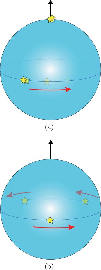
Figure 1. Illustration of two simple stars'structures. (a)When there are two stars fixed at the north pole and one star travels along the equator. (b)When the three stars locate at the equator uniformly and rotate along the equator together. |
When there are two stars fixed in the north pole and one star travels along the equator (figure 1(a)), i.e. ${\vec{n}}_{1}={\vec{n}}_{2}=(0,0,1)$, ${\vec{n}}_{3}=(\cos \omega t,\sin \omega t,0)$, we are interested in Qωω. In this case, the QGT does not have the antisymmetric part, and the symmetric part is its real part, which is the quantum Fisher information for ω. The QGT reads
$\begin{eqnarray}{Q}_{\omega \omega }=\displaystyle \frac{3{t}^{2}}{16}.\end{eqnarray}$
The second interesting example is the GHZ-type states [13], where the three stars locate at the equator uniformly and rotate along the equator together (figure 1(b)). The stars hold the relation ${\vec{n}}_{1}+{\vec{n}}_{2}+{\vec{n}}_{3}\,=\,0$ all the time and the QGT with respect to rotating frequency is
$\begin{eqnarray}{Q}_{\omega \omega }=\displaystyle \frac{9{t}^{2}}{4}.\end{eqnarray}$
Since the real part of QGT gives the quantum Fisher information, this means the second example is better to estimate the rotating frequency than the first one.
4. Applications to the LMG model
In order to show that our results are convincing, we examine a simple example and illustrate how the MSR works. The research on the QGT of the LMG model has attracted much attention [37–39]. Now we consider the anisotropic case of the LMG model [40]:
$\begin{eqnarray}H=\alpha {J}_{x}^{2}+\beta {J}_{z},\end{eqnarray}$
where α < 0 and β < 0.We are concerned with the spin-$\tfrac{3}{2}$ case. This Hamiltonian can be written as the following matrix of the equation (39 ) under the bases
$\begin{eqnarray*}\begin{array}{l}\left\{| 0\rangle =| \uparrow \uparrow \uparrow \rangle ,\,| 1\rangle =\displaystyle \frac{| \downarrow \downarrow \uparrow \rangle +| \downarrow \uparrow \downarrow \rangle +| \uparrow \downarrow \downarrow \rangle }{\sqrt{3}},\right.\\ | 2\rangle =\left.\displaystyle \frac{| \downarrow \uparrow \uparrow \rangle +| \uparrow \downarrow \uparrow \rangle +| \uparrow \uparrow \downarrow \rangle }{\sqrt{3}},\,| 3\rangle =| \downarrow \downarrow \downarrow \rangle \right\},\end{array}\end{eqnarray*}$
and $\begin{eqnarray}H=\left(\begin{array}{cccc}\displaystyle \frac{3}{4}\alpha +\displaystyle \frac{3}{2}\beta & \displaystyle \frac{\sqrt{3}}{2}\alpha & 0 & 0\\ \displaystyle \frac{\sqrt{3}}{2}\alpha & \displaystyle \frac{7}{4}\alpha -\displaystyle \frac{1}{2}\beta & 0 & 0\\ 0 & 0 & \displaystyle \frac{7}{4}\alpha +\displaystyle \frac{1}{2}\beta & \displaystyle \frac{\sqrt{3}}{2}\alpha \\ 0 & 0 & \displaystyle \frac{\sqrt{3}}{2}\alpha & \displaystyle \frac{3}{4}\alpha -\displaystyle \frac{3}{2}\beta \end{array}\right).\end{eqnarray}$
Then we take care of the two lower eigenstates. The first one is in the subspace of ∣0⟩, ∣1⟩: $\begin{eqnarray}| {\chi }_{1}\rangle =a| \uparrow \uparrow \uparrow \rangle +\displaystyle \frac{b}{\sqrt{3}}(| \downarrow \downarrow \uparrow \rangle +| \downarrow \uparrow \downarrow \rangle +| \uparrow \downarrow \downarrow \rangle ),\end{eqnarray}$
where the coefficients $\begin{eqnarray}a=-\displaystyle \frac{{\delta }_{1}}{\alpha \sqrt{3+\tfrac{{\delta }_{1}^{2}}{{\alpha }^{2}}}},\,b=\displaystyle \frac{1}{\sqrt{1+\tfrac{{\delta }_{1}^{2}}{3{\alpha }^{2}}}},\end{eqnarray}$
in which ${\delta }_{1}\,=\,2\sqrt{{\alpha }^{2}-\alpha \beta +{\beta }^{2}}+\alpha -2\beta \gt 0$. Since in this case, ${C}_{\tfrac{3}{2}}=a$ and ${C}_{-\tfrac{1}{2}}=b$, the Majorana star equation exhibits $\begin{eqnarray}\displaystyle \frac{a}{\sqrt{6}}{z}^{3}+\displaystyle \frac{b}{\sqrt{2}}z=0.\end{eqnarray}$
The Majorana stars are obtained $z\,=\,0,\pm {\rm{i}}\sqrt{\tfrac{\sqrt{3}b}{a}}$. The spherical coordinates of the three stars are $(0,\sin \theta ,\cos \theta ),(0,-\sin \theta ,\cos \theta )\,\mathrm{and}\,(0,0,1)$, where $\tan \tfrac{\theta }{2}=\sqrt{\tfrac{\sqrt{3}b}{a}}$. Then we substitute these vectors in the expression of the real and imaginary part of QGT, we obtain the explicit form of QGT: $\begin{eqnarray}\begin{array}{rcl}{Q}_{\alpha \beta } & = & \displaystyle \frac{3\,{\partial }_{\alpha }\theta \,{\partial }_{\beta }\theta {\sin }^{2}\theta }{{(3+2\,\cos \theta +\cos (2\theta ))}^{2}}\\ & = & \displaystyle \frac{{\partial }_{\alpha }b\,{\partial }_{\beta }b}{1-{b}^{2}}=-\displaystyle \frac{3\alpha \beta }{16{\left({\alpha }^{2}-\alpha \beta +{\beta }^{2}\right)}^{2}},\end{array}\end{eqnarray}$
$\begin{eqnarray}{Q}_{\alpha \alpha }=\displaystyle \frac{{({\partial }_{\alpha }b)}^{2}}{1-{b}^{2}}=\displaystyle \frac{3{\beta }^{2}}{16{\left({\alpha }^{2}-\alpha \beta +{\beta }^{2}\right)}^{2}},\end{eqnarray}$
$\begin{eqnarray}{Q}_{\beta \beta }=\displaystyle \frac{{({\partial }_{\beta }b)}^{2}}{1-{b}^{2}}=\displaystyle \frac{3{\alpha }^{2}}{16{\left({\alpha }^{2}-\alpha \beta +{\beta }^{2}\right)}^{2}}.\end{eqnarray}$
The relation between the QGT and the parameters is shown in figure 2. The QGT only becomes divergent when α = β = 0. This is obvious since the Hamiltonian vanishes in this case, which means the trivial degeneracy of energy levels.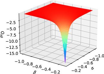
Figure 2. Qαβ of the first lower eigenstate of LMG model for spin-3/2. It becomes divergent when α = β = 0. |
Similarly, the second lower eigenstate is in the subspace of ∣2⟩, ∣3⟩:
$\begin{eqnarray}| {\chi }_{2}\rangle =\displaystyle \frac{c}{\sqrt{3}}(| \downarrow \uparrow \uparrow \rangle +| \uparrow \downarrow \uparrow \rangle +| \uparrow \uparrow \downarrow \rangle )+d| \downarrow \downarrow \downarrow \rangle ,\end{eqnarray}$
where $\begin{eqnarray}c=-\displaystyle \frac{{\delta }_{2}}{\alpha \sqrt{3+\tfrac{{\delta }_{2}^{2}}{{\alpha }^{2}}}},\,d=\displaystyle \frac{1}{\sqrt{1+\tfrac{{\delta }_{2}^{2}}{3{\alpha }^{2}}}},\end{eqnarray}$
in which ${\delta }_{2}\,=\,2\sqrt{{\alpha }^{2}+\alpha \beta +{\beta }^{2}}-\alpha -2\beta \gt 0$. The Majorana stars are similarly obtained as $(0,\sin \phi ,\cos \phi ),(0,-\sin \phi ,\cos \phi )\,\mathrm{and}\,(0,0,-1)$, where $\tan \tfrac{\phi }{2}=\sqrt{\tfrac{d}{\sqrt{3}c}}$. The QGT reads $\begin{eqnarray}\begin{array}{rcl}{Q}_{\alpha \beta } & = & \displaystyle \frac{3\,{\partial }_{\alpha }\phi \,{\partial }_{\beta }\phi {\sin }^{2}\phi }{{(3-2\,\cos \phi +\cos (2\phi ))}^{2}}\\ & = & -\displaystyle \frac{3\alpha \beta }{16{\left({\alpha }^{2}+\alpha \beta +{\beta }^{2}\right)}^{2}},\end{array}\end{eqnarray}$
$\begin{eqnarray}{Q}_{\alpha \alpha }=\displaystyle \frac{{({\partial }_{\alpha }c)}^{2}}{1-{c}^{2}}=\displaystyle \frac{3{\beta }^{2}}{16{\left({\alpha }^{2}+\alpha \beta +{\beta }^{2}\right)}^{2}},\end{eqnarray}$
$\begin{eqnarray}{Q}_{\beta \beta }=\displaystyle \frac{{({\partial }_{\beta }c)}^{2}}{1-{c}^{2}}=\displaystyle \frac{3{\alpha }^{2}}{16{\left({\alpha }^{2}+\alpha \beta +{\beta }^{2}\right)}^{2}}.\end{eqnarray}$
The divergence is similar to the first case, and this example testifies the validity of our results.5. Extensions to arbitrary spin
After discussing the spin-1 and spin-3/2 cases, we will give some properties of arbitrary spin state. For arbitrary spin, the MSR for QGT is difficult to obtain, but we can know it in some simple situation.
For example, the QGT of the ferromagnetic state, in which all stars coincide at one point and will remain coincident for a moment: $({\vec{n}}_{1}={\vec{n}}_{2}=\cdots ={\vec{n}}_{N}=\vec{n})$, can be easily calculated as51 )52 ). However, the process is tedious and needs to solve the series. The direct calculation verifies the correctness of the equation (53 ).
$\begin{eqnarray}{Q}_{\alpha \beta }=\displaystyle \frac{N}{4}({\partial }_{\alpha }\vec{n}\cdot {\partial }_{\beta }\vec{n}+{\rm{i}}\vec{n}\cdot {\partial }_{\alpha }\vec{n}\times {\partial }_{\beta }\vec{n}).\end{eqnarray}$
The typical example is still the spin coherent state for the arbitrary spin $\begin{eqnarray}| \zeta {\rangle }_{j}={{\rm{e}}}^{\zeta {\hat{J}}_{+}}| J,-J\rangle ,\end{eqnarray}$
where $\zeta =\tan \tfrac{\theta }{2}{{\rm{e}}}^{{\rm{i}}\phi }$. All the Majorana stars converge at the point $(\sin \theta \cos \phi ,\sin \theta \sin \phi ,\cos \theta )$. If we set the parameters α = θ and β = φ, the QGT of the spin coherent state is easily obtained from the equation ( $\begin{eqnarray}{Q}_{\theta \phi }=\displaystyle \frac{{\rm{i}}}{2}J\sin \theta .\end{eqnarray}$
The QGT possesses rotating invariance with respect to φ. Since its real part vanishes, the spin coherent state cannot be used to measure θ and φ from the perspective of quantum metrology. The same result can be also derived from equation (We begin to discuss the second important case for an arbitrary spin. When it has J + m coincident points at $\vec{n}=(\sin \theta \cos \phi ,\sin \theta \sin \phi ,\cos \theta )$, and J − m coincident antipodal points at $-\vec{n}$, the QGT reads53 ). In particular, when there are nearly one half of the stars remain to be $\vec{n}$ and the others are $-\vec{n}$, the result can be obtained from equation (54 ). For example, if there are 2N stars, N of which are $\vec{n}$ while the others are $-\vec{n}$, i.e. m = 0 and J = N is integer, the MSR of QGT becomes
$\begin{eqnarray}{Q}_{\alpha \beta }=\displaystyle \frac{{J}^{2}+J-{m}^{2}}{2}{\partial }_{\alpha }\vec{n}\cdot {\partial }_{\beta }\vec{n}+{\rm{i}}\displaystyle \frac{m}{2}\vec{n}\cdot {\partial }_{\alpha }\vec{n}\times {\partial }_{\beta }\vec{n}.\end{eqnarray}$
The corresponding state is a spin in a uniform magnetic field [13]: $\begin{eqnarray}| m;\theta ,\phi \rangle ={{\rm{e}}}^{-{\rm{i}}{\hat{J}}_{z}\phi }{{\rm{e}}}^{-{\rm{i}}{\hat{J}}_{y}\theta }{{\rm{e}}}^{{\rm{i}}{\hat{J}}_{z}\phi }| {Jm}\rangle .\end{eqnarray}$
If we still choose θ and φ as parameters, the QGT of this state becomes $\begin{eqnarray}{Q}_{\theta \phi }=\displaystyle \frac{{\rm{i}}}{2}m\sin \theta ,\end{eqnarray}$
in which the well-known Berry curvature emerges. When m = J, it recovers the expression of equation ( $\begin{eqnarray}{Q}_{\alpha \beta }=\displaystyle \frac{N(N+1)}{2}{\partial }_{\alpha }\vec{n}\cdot {\partial }_{\beta }\vec{n}=\displaystyle \frac{J(J+1)}{2}{\partial }_{\alpha }\vec{n}\cdot {\partial }_{\beta }\vec{n}.\end{eqnarray}$
The imaginary part, or the Berry curvature, vanishes in this case. However, the real part is not zero in general, unless we take θ and φ as parameters. When there are 2N + 1 stars, N + 1 of which are $\vec{n}$ while the others are $-\vec{n}$, i.e. $m=\tfrac{1}{2}$ and $J\,=\,N+\tfrac{1}{2}$ is half-integer, $\begin{eqnarray}\begin{array}{rcl}{Q}_{\alpha \beta } & = & \displaystyle \frac{2{N}^{2}+4N+1}{4}{\partial }_{\alpha }\vec{n}\cdot {\partial }_{\beta }\vec{n}+\displaystyle \frac{{\rm{i}}}{4}\vec{n}\cdot {\partial }_{\alpha }\vec{n}\times {\partial }_{\beta }\vec{n}\\ & = & \displaystyle \frac{4J(J+1)-1}{8}{\partial }_{\alpha }\vec{n}\cdot {\partial }_{\beta }\vec{n}+\displaystyle \frac{{\rm{i}}}{4}\vec{n}\cdot {\partial }_{\alpha }\vec{n}\times {\partial }_{\beta }\vec{n}.\end{array}\end{eqnarray}$
The imaginary part identifies with that of one-star situation, thus resulting to the same geometric quantities such as the Berry phase or Chern number under this configuration.The third special case is an extension of the first case in section 3.2 . We consider the situation where N − 1 stars are always located at ${\vec{n}}_{0}$ and the remaining one star $\vec{n}$ move in a plane perpendicular to ${\vec{n}}_{0}$. The QGT is36 ) when N = 3 and α = β = ω. It is provoking that the Qαβ does not depend on the stationary star ${\vec{n}}_{0}$. This reminds us of the rotation invariance of the MSR for the QGT, which originates from the gauge invariance of the QGT. Then we can draw the following proposition.
$\begin{eqnarray}{Q}_{\alpha \beta }=\displaystyle \frac{N}{{(N+1)}^{2}}{\partial }_{\alpha }\vec{n}\cdot {\partial }_{\beta }\vec{n}.\end{eqnarray}$
It reduces to the equation (The parameter-independent global rotation of the Majorana stars will not change the MSR for QGT.
For the parameter-independent global rotation, we can write the corresponding unnormalized state as
$\begin{eqnarray}\begin{array}{rcl}| \vec{u}^{\prime} \rangle & \equiv & {\boldsymbol{u}}| \vec{u}\rangle \\ & \equiv & \displaystyle \frac{1}{\sqrt{N!}}\sum _{P}U| {u}_{P(1)}\rangle \otimes U| {u}_{P(2)}\rangle \otimes \cdots U| {u}_{P(N)}\rangle \\ & = & (U\otimes U\otimes \cdots U)| \vec{u}\rangle ,\end{array}\end{eqnarray}$
where U is a two-dimensional unitary matrix and ${\boldsymbol{u}}$ is the direct product of N two-dimensional unitary matrices U. Since ${\boldsymbol{u}}$ is also a unitary matrix and parameter-independent, it does not influence the result of QGT in equation (This proposition can help us when the Majorana stars do not possess certain symmetry. We can rotate all the stars to some special positions to simplify the calculation. And it also explains the reason why the QGT does not contain vectors of those stationary stars.
We can also deduce from the above proposition that when all the stars fix on a parameter-independent plane, they can be rotated to the x–z plane, which makes its Berry curvature vanish, such as the examples in section 4 .
6. Conclusion
The MSR has been a promising tool to study the many-body phenomena and higher spin states. In this article, we use this representation to study the quantum geometric tensor. The latter is vital in the research of quantum phase transition and quantum topological aspects. We give the results of the QGT up to spin-3/2 states and a general expression of arbitrary spin remains to be found. The result of MSR for QGT is already complex in the spin-3/2 case, and the higher spin situation will be difficult to obtain. However, the results (34 ) and (35 ) are easy to calculate on a computer once we obtain the explicit form of MSR. From the results of section 4 , we can see that some special states are represented as simple star structures in the MSR, which simplifies the calculation of the QGT of MSR. Some chosen parameters, such as θ and φ, make the real part or the imaginary part vanish, thus leading to the loss of metrology capability or geometric properties.
There are also some questions to be addressed. For example, the general formulation of MSR for QGT to arbitrary spin is needed. There is no doubt that the interaction between Majorana stars will become more intricate in higher spin states. Moreover, the deep connection between the MSR for QGT and the topological quantities [11] remains to be explored. Indeed the Majorana stars have been proven to facilitate the definition of the topological quantities, which somehow provide surprisingly useful results [10]. Besides the use of the MSR for metric tensor in the spinor condensates [4], other applications of MSR for the metric tensor in topological quantum numbers are still an open question. As a whole, the MSR for the QGT will find more applications in topological physics. It is also interesting to use MSR to study the band topological problems. We believe our results will pave the way to further research on relations between the topological quantum mechanics and MSR.