


1. Introductions
Today we are entering a new Universe of precise cosmic progress. The cosmological parameters are tightly constrained by observations such as type Ia supernovae (SNIa) [1], baryon acoustic oscillations (BAO) [2], cosmic microwave background (CMB) [3], gravitational lensing systems [4], gravitational waves [5]. Contrary to the standard cosmological model, observations have shown that the Universe is expanding in an accelerated way. This late-time acceleration era is known as the dark energy (DE) era, and until today remains a mystery on its driving force. The approach of Λ-cold dark matter (ΛCDM) cosmology is probably the best fitted cosmological model in which the cosmological constant Λ accelerates the expansion of our Universe. This approach is established based on the observational results. Different kinds of theoretical models have already been implemented to interpret the accelerating Universe. Comprehensive studies have been conducted on these subjects in [6–8]. Due to the complex nature of the acceleration of the Universe and the fact that their underlying physical mechanism has not yet been fully understood, different methods are widely applied in order to study them.
Over the last twenty years, DE models have been proposed to explain the acceleration of the Universe (see [9–11]). Holographic dark energy (HDE) models are established on the holographic principle [12]. The approach of the HDE model is developed to describe the late-time acceleration, quantitatively [10, 13–17]. It is also in agreement with observational data [18–22]. Therefore, many extensions of the basic scenario have appeared in the related context, mainly based on the use of different horizons as the largest distance (i.e. the radius of the Universe) [23–31]. Later, Gao et al suggested that the DE density might be inversely proportional to the Ricci scalar curvature (R) [32]. This model was called the Ricci dark energy (RDE) model. In the RDE model, the future event horizon has been replaced by the inverse of the Ricci scalar curvature. Furthermore, the RDE models have been developed into well-known models such as the extended RDE [33]. The evolution of the various cosmological parameters in the RDE model were studied in the light of supernovae, SDSS and recent Planck data [34]. Researchers have shown the RDE model is suitable for describing the current acceleration of the Universe [35–37].
Besides the DE problem, the concept of anisotropy is also adopted by current cosmology. The isotropic Friedmann–Robertson–Walker (FRW) model alongside the spatially homogeneous model describe the nature of the current Universe, completely. But, the recent observational data supports the existence of an anisotropic phase in the past eras of the Universe [38]. This fact confirmed that the early anisotropic Universe turned into the present isotropic Universe [39, 40]. The Bianchi type cosmological models represent the homogeneous and anisotropic Universe, where their isotropic nature of them may also be studied with the passage of time. The approach of the Bianchi I (BI) model utilizes semi-analytical calculations. The basic effects available in anisotropic models are also captured in the BI model by considering important common properties between them and direction-dependent expansion rates. The anisotropic Bianchi type cosmological model was investigated from different perspectives by many authors [41–45]. Wang et al used the Joint Light curve Analysis (JLA) sample to constrain the anisotropic Universe with the BI model and found that the model was consistent with the isotropic Universe [46]. Hossienkhani et al have investigated an anisotropic BI Universe in the DE models [47–49]. They studied different observational data and evolutionary stages of cosmic expansion. Some useful applications of the anisotropic Universe compatible with astrophysical observations are described in [50–56].
We develop the evolution of RDE in an anisotropic BI model of the Universe by considering the latest observational data. In section 2 the metric and the field equations for the RDE model are described. Section 3 is devoted to reviewing the observational data and the applied techniques. The results are discussed in section 4 . In section 5 , the effects of anisotropy are investigated on the evolution of the Hubble parameter, the equation of state (EoS) parameter and the deceleration parameter. Finally, the conclusion is presented in section 6 .
2. Metric and the cosmological model
As discussed in the introduction, we shall restrict our attention to space-times of BI model. The line element in such a spacetime is given by1 ), can be written as follows4 ) for space-time (1 ) are given by [57, 58]10 ) the mean Hubble parameter H(z) is derived as follows14 ) that the RDE contains three terms: the first one behaves like cold dark matter, the second one behaves like anisotropy DE and the last term behaves like an exotic energy component whose properties are determined by the parameter α. Requiring the consistency of (13 ) at z = 0, gives10 ) and (11 ), we can express ω(z) and q(z) in terms of H(z), dH/dz, ${{\rm{\Omega }}}_{{\sigma }_{0}}$ and ${{\rm{\Omega }}}_{{m}_{0}}$ 20 ) can be useful in characterizing the expansion history but it should not be interpreted as a property of an energy substance. When the anisotropy density goes to zero, i.e. σ0 → 0, and ${{\rm{\Omega }}}_{{\sigma }_{0}}\to 0$ (i.e. spatially isotropic Universe), the EoS parameter (19 ) is reduced to that of the [59–64].
$\begin{eqnarray}{{\rm{d}}{s}}^{2}={{\rm{d}}{t}}^{2}-{A}^{2}(t){{\rm{d}}{x}}^{2}-{B}^{2}(t){{\rm{d}}{y}}^{2}-{C}^{2}(t){{\rm{d}}{z}}^{2},\end{eqnarray}$
where A, B and C are the functions of ‘t'alone. It is worth noting that in BI case, the average scale factor is defined as $a={\left({ABC}\right)}^{1/3}$. The energy–momentum tensors of pressureless matter and RDE are given by, respectively $\begin{eqnarray}{T}_{{ij}}^{m}={\rho }_{m}{u}_{i}{u}_{j},\end{eqnarray}$
$\begin{eqnarray}{T}_{{ij}}^{\mathrm{de}}=({\rho }_{\mathrm{de}}+{p}_{\mathrm{de}}){u}_{i}{u}_{j}-{g}_{{ij}}{p}_{\mathrm{de}},\end{eqnarray}$
where ρm is matter energy density, ρde and pde are the energy-density and the pressure of RDE model, respectively. Also ui is 4-velocity of the fluid which is normalized as uiui = 1. Einstein's field equations $\begin{eqnarray}{R}_{{ij}}-\displaystyle \frac{1}{2}{{Rg}}_{{ij}}=\displaystyle \frac{1}{{M}_{p}^{2}}\left({T}_{{ij}}^{m}+{T}_{{ij}}^{\mathrm{de}}\right),\end{eqnarray}$
where ${M}_{P}^{2}=\tfrac{1}{8\pi G}$ is the reduced Planck mass. The energy-density ρde of the RDE takes the form [32] $\begin{eqnarray}{\rho }_{\mathrm{de}}=3\alpha {M}_{p}^{2}(\dot{H}+2{H}^{2}),\end{eqnarray}$
where α is a dimensionless constant, H is the mean Hubble parameter and $\dot{H}$ is its derivative with respect to cosmic time. In a BI Universe, the important physical quantities like the spatial volume V, the expansion scalar θ, the mean Hubble expansion factor H and the shear scalar σ2 for the metric ( $\begin{eqnarray}V={a}^{3}={ABC},\end{eqnarray}$
$\begin{eqnarray}\theta ={u}_{;i}^{i}=\displaystyle \frac{\dot{A}}{A}+\displaystyle \frac{\dot{B}}{B}+\displaystyle \frac{\dot{C}}{C},\end{eqnarray}$
$\begin{eqnarray}H=\displaystyle \frac{\dot{a}}{a}=\displaystyle \frac{1}{3}\left(\displaystyle \frac{\dot{A}}{A}+\displaystyle \frac{\dot{B}}{B}+\displaystyle \frac{\dot{C}}{C}\right),\end{eqnarray}$
$\begin{eqnarray}{\sigma }^{2}=\displaystyle \frac{1}{2}{\sigma }_{{ij}}{\sigma }^{{ij}}=\displaystyle \frac{1}{2}\left({\left(\displaystyle \frac{\dot{A}}{A}\right)}^{2}+{\left(\displaystyle \frac{\dot{B}}{B}\right)}^{2}+{\left(\displaystyle \frac{\dot{C}}{C}\right)}^{2}\right)-\displaystyle \frac{1}{6}{\theta }^{2},\end{eqnarray}$
where an overdot denotes derivative with respect to cosmic time t. The field equation ( $\begin{eqnarray}3{H}^{2}-{\sigma }^{2}=\displaystyle \frac{1}{{M}_{p}^{2}}({\rho }_{m}+{\rho }_{\mathrm{de}}),\end{eqnarray}$
$\begin{eqnarray}2\dot{H}+3{H}^{2}+{\sigma }^{2}=-\displaystyle \frac{1}{{M}_{p}^{2}}\,{p}_{\mathrm{de}}.\end{eqnarray}$
Note that the isotropic case now corresponds to σ = 0. The density parameters Ωm, Ωde and Ωσ are defined by $\begin{eqnarray}{{\rm{\Omega }}}_{m}=\displaystyle \frac{{\rho }_{m}}{3{M}_{p}^{2}{H}^{2}},\,\,{{\rm{\Omega }}}_{\mathrm{de}}=\displaystyle \frac{{\rho }_{\mathrm{de}}}{3{M}_{p}^{2}{H}^{2}},\,\,{{\rm{\Omega }}}_{\sigma }=\displaystyle \frac{{\sigma }^{2}}{3{H}^{2}}.\end{eqnarray}$
Therefore, using equation ( $\begin{eqnarray}\begin{array}{rcl}{H}^{2}(z) & = & {H}_{0}^{2}(z)\left[{{\rm{\Omega }}}_{{m}_{0}}{\left(1+z\right)}^{3}+{{\rm{\Omega }}}_{{\sigma }_{0}}{\left(1+z\right)}^{6}\right.\\ & & +\displaystyle \frac{\alpha }{2-\alpha }{{\rm{\Omega }}}_{{m}_{0}}{\left(1+z\right)}^{3}-\displaystyle \frac{\alpha }{1+\alpha }{{\rm{\Omega }}}_{{\sigma }_{0}}{\left(1+z\right)}^{6}\\ & & \left.+{f}_{0}{\left(1+z\right)}^{4-\tfrac{2}{\alpha }}\right],\end{array}\end{eqnarray}$
where $a={\left(1+z\right)}^{-1}$, ${f}_{0}=1-{{\rm{\Omega }}}_{{\sigma }_{0}}/(1+\alpha )$ $-2{{\rm{\Omega }}}_{{m}_{0}}/(2-\alpha )$ and Ωde is defined as the dimensionless energy density of RDE in term of redshift z $\begin{eqnarray}\begin{array}{rcl}{{\rm{\Omega }}}_{\mathrm{de}}(z) & = & \displaystyle \frac{\alpha }{2-\alpha }{{\rm{\Omega }}}_{{m}_{0}}{\left(1+z\right)}^{3}\\ & & -\displaystyle \frac{\alpha }{1+\alpha }{{\rm{\Omega }}}_{{\sigma }_{0}}{\left(1+z\right)}^{6}+{f}_{0}{\left(1+z\right)}^{4-\tfrac{2}{\alpha }}.\end{array}\end{eqnarray}$
In the case of α = 2 is not a viable DE model. Once one has α ≠ 2, it can be seen from equation ( $\begin{eqnarray}{{\rm{\Omega }}}_{{m}_{0}}+{{\rm{\Omega }}}_{{\mathrm{de}}_{0}}=1-{{\rm{\Omega }}}_{{\sigma }_{0}}.\end{eqnarray}$
The conservation law for matter, RDE and shear scalar are given by $\begin{eqnarray}{\dot{\rho }}_{m}+3H{\rho }_{m}=0,\end{eqnarray}$
$\begin{eqnarray}{\dot{\rho }}_{\mathrm{de}}+3H(1+{\omega }_{\mathrm{de}}){\rho }_{\mathrm{de}}=0,\end{eqnarray}$
$\begin{eqnarray}\dot{\sigma }+3H\sigma =0,\end{eqnarray}$
in which ωde = pde/ρde represents the RDE EoS parameter. Now we describe the EoS ωde(z) and the deceleration parameter $q(z)=-1+(1+z)\tfrac{{\rm{d}}\mathrm{ln}H}{{\rm{d}}{z}}$ which in general depends on the redshift z. Using the BI equations ( $\begin{eqnarray}{\omega }_{\mathrm{de}}(z;{ \mathcal P })=\displaystyle \frac{\tfrac{2}{3}(1+z)\tfrac{{\rm{d}}\mathrm{ln}H}{{\rm{d}}{z}}-{{\rm{\Omega }}}_{{\sigma }_{0}}{\left(1+z\right)}^{6}{\left(\tfrac{{H}_{0}}{H}\right)}^{2}-1}{1-{\left(\tfrac{{H}_{0}}{H}\right)}^{2}\left[{{\rm{\Omega }}}_{{m}_{0}}{\left(1+z\right)}^{3}+{{\rm{\Omega }}}_{{\sigma }_{0}}{\left(1+z\right)}^{6}\right]},\end{eqnarray}$
$\begin{eqnarray}\begin{array}{rcl}q(z;{ \mathcal P }) & = & \displaystyle \frac{1}{2}+\displaystyle \frac{3}{2}\omega (z)\left[1-{\left(\displaystyle \frac{{H}_{0}}{H}\right)}^{2}\left({{\rm{\Omega }}}_{{m}_{0}}{\left(1+z\right)}^{3}\right.\right.\\ & & \left.\left.+{{\rm{\Omega }}}_{{\sigma }_{0}}{\left(1+z\right)}^{6}\right)\right]+\displaystyle \frac{3}{2}{{\rm{\Omega }}}_{{\sigma }_{0}}{\left(1+z\right)}^{6}{\left(\displaystyle \frac{{H}_{0}}{H}\right)}^{2},\end{array}\end{eqnarray}$
being ${ \mathcal P }=({{\rm{\Omega }}}_{{m}_{0}};{{\rm{\Omega }}}_{{\sigma }_{0}};{H}_{0};\alpha )$, the free parameter vector to be fitted by the data. We use the ${ \mathcal P }$ mean values in the last expression to reconstruct the EoS parameter and the deceleration parameter. We also investigate whether the RDE model is consistent with a late cosmic acceleration. Regarding the validity of generalized BI equations in modified gravity models, equation (3. Observational analysis
Following the derivation of the Hubble parameter obtained in equation (13 ), here we estimate the best fit of the model parameters ${{\rm{\Omega }}}_{{m}_{0}}$, ${{\rm{\Omega }}}_{{\sigma }_{0}}$, H0 and α with the combined data set consisting of the supernovae type Ia from the Pantheon Sample [1] and observational Hubble data. Using the χ2 minimization technique, we estimate the model parameters, which will give us a reasonable idea about the evolutionary status of the Universe in RDE of BI model. In order to figure out the observational constraints, we employ the maximum likelihood estimation (MLE) method.
3.1. Type Ia supernovae
We use the most updated compilation of SNIa, the Pantheon Sample, which contains a set of 1048 spectroscopically confirming SNIa [1] ranging from redshift 0.01 to 2.3, along with a covariance matrix (including statistical and systematic errors). The Pantheon catalog contains measurements of peak magnitudes in the B-band's rest frame, mB, which are related to the distance modulus with μobs = mB − M, where M is a nuisance parameter corresponding to the absolute B-band magnitude of a fiducial SNIa. Following [65], we define the theoretical magnitude of a supernova to be
$\begin{eqnarray}{\mu }_{\mathrm{th}}=5\mathrm{log}{D}_{L}(z)+{\mu }_{0},\end{eqnarray}$
where ${\mu }_{0}=42.384-5\mathrm{log}h$ with h the Hubble constant H0 in units of 100 km/s/Mpc and the Hubble-free luminosity distance DL is $\begin{eqnarray}{D}_{L}(z)=(1+{z}_{\mathrm{hel}}){\int }_{0}^{{z}_{\mathrm{cmb}}}\displaystyle \frac{{\rm{d}}\tilde{z}}{E(\tilde{z})}.\end{eqnarray}$
In this equation, zhel is the heliocentric redshift, and zcmb is the CMB-frame redshift. Finally, the corresponding likelihood reads $\begin{eqnarray}{{ \mathcal L }}_{\mathrm{SNIa}}({ \mathcal P };M)\sim \exp \left(-\displaystyle \frac{1}{2}\sum _{i=1}^{1048}{m}_{i}{{ \mathcal C }}_{\mathrm{cov}}^{-1}{m}_{i}^{\dagger }\right),\end{eqnarray}$
where mi = μobs,i − μth(zi). Finally, the marginalized χ2 function of SNIa can be written as [66–68] $\begin{eqnarray}{\chi }_{\mathrm{SNIa}}^{2}=\sum _{i=1}^{1048}\displaystyle \frac{{\left[{\mu }_{\mathrm{obs},i}-{\mu }_{\mathrm{th}}({z}_{i})\right]}^{2}}{\sigma {{\prime} }_{\mu ,i}^{2}+\sigma {{\prime} }_{\mathrm{int}}^{2}+\sigma {{\prime} }_{\mathrm{lens}}^{2}},\end{eqnarray}$
where ${\mu }_{\mathrm{obs},i}={\mu }_{\mathrm{SN}}(M;{z}_{i})$, ${\mu }_{\mathrm{th}}({z}_{i})=\mu ({{\rm{\Omega }}}_{{m}_{0}},{{\rm{\Omega }}}_{{\sigma }_{0}},{H}_{0};z)$. $\sigma {{\prime} }_{\mu ,i}$, $\sigma {{\prime} }_{\mathrm{int}}$ and $\sigma {{\prime} }_{\mathrm{lens}}$ are the standard errors of the peak magnitude, the intrinsic dispersion error of each SNIa and the intrinsic scatter due to gravitational lensing, respectively.3.2. Hubble parameter data
In addition to the SNIa observations, we also considered observational Hubble data from the cosmic chronometers (CC) and baryon acoustic oscillations (BAO) measurements. CC are measurements of the Hubble rate, based on the estimation of the differential age of passive evolving galaxies [69]. In the second method, called ‘BAO measurements', the Hubble parameter measurements depend on BAO scale [70]. In this work, we considered the updated list compiled by Maga$\tilde{n}$ea et al [71] which contains 31 points from CC, 20 points from BAO measurements and also a data point based on the local value of Hubble parameter H0 provided from results (R19) [72]. The likelihood function based on the maximum likelihood method is as follows:
$\begin{eqnarray}{{ \mathcal L }}_{\mathrm{Hubble}}({ \mathcal P })\sim \exp \left(-\displaystyle \frac{1}{2}\sum _{i=1}^{52}\displaystyle \frac{{\left(H{\left({z}_{i}\right)}_{\mathrm{th}}-H(\mathrm{obs},i)\right)}^{2}}{{\sigma }_{i}^{{\prime} 2}}\right),\end{eqnarray}$
where $\sigma {{\prime} }_{i}$ denote the standard error in experimental values of Hubble's function H. The χ2 function is defined as follows: $\begin{eqnarray}{\chi }_{\mathrm{Hubble}}^{2}=\sum _{i=1}^{52}\displaystyle \frac{{\left[H{\left({z}_{i}\right)}_{\mathrm{th}}-H(\mathrm{obs},i)\right]}^{2}}{{\sigma }_{i}^{{\prime} 2}}.\end{eqnarray}$
3.3. Joint analysis
We employ N cosmological datasets to obtain the joint observational constraints on the cosmological scenario. We first introduce the total likelihood function as
$\begin{eqnarray}{{ \mathcal L }}_{\mathrm{tot}}({ \mathcal P })=\prod _{n=1}^{N}{{ \mathcal L }}_{i}.\end{eqnarray}$
There is no correlation between the data sets used. The total χ2 function is then given by $\begin{eqnarray}{\chi }_{\mathrm{tot}}^{2}={\chi }_{\mathrm{SNIa}}^{2}+{\chi }_{\mathrm{Hubble}}^{2}.\end{eqnarray}$
For the combined dataset (Pantheon + H(z)), we estimate the best-fit values of the model parameters by minimizing χ2. Then, we use the maximum likelihood method and take the combined likelihood function as ${ \mathcal L }({ \mathcal P })={{\rm{e}}}^{-{\chi }^{2}/2}$. The best-fit parameter values ${ \mathcal P }$ are those that minimize the likelihood function. We can now plot the contours for different confidence levels, e.g. $1\sigma ^{\prime} (68.3 \% )$ with Δχ2 = 2.3 and $2\sigma ^{\prime} (95.4 \% )$ with Δχ2 = 6.17 where ${\rm{\Delta }}{\chi }^{2}={\chi }^{2}({ \mathcal P })-{\chi }_{\min }^{2}({ \mathcal P })$ and ${\chi }_{\min }^{2}$ is the minimum value of χ2. An important quantity that could be used for the data fitting process as ${\chi }_{\mathrm{dof}}^{2}={\chi }_{\min }^{2}/({N}_{\mathrm{tot}}+k)$, where ‘dof'is the degree of freedom, Ntot is the total observational data and k is the free parameters. If Δχ2 ≤ 1, then the fit is good and the data are consistent with the considered model. In what follows, we discuss the results obtained from the statistical analysis of the above mentioned datasets.4. Results and observational constraints
RDE in BI model has five unknown parameters to be estimated from H(z), Pantheon, and their joint combination. The base parameters set for this model is
$\begin{eqnarray}{ \mathcal P }=\{{{\rm{\Omega }}}_{{m}_{0}},{{\rm{\Omega }}}_{{\sigma }_{0}},\alpha ,{H}_{0};M\}.\end{eqnarray}$
To examine the validity of the model on fitting datasets, we calculate ${\chi }_{\mathrm{dof}}^{2}$ with N = 1048, 52, 1100 represents the data set points. We notice that the model is compatible with the reasonable value of the goodness of freedom (dof). In table 1, we show values ${{\rm{\Omega }}}_{{m}_{0}},\,{{\rm{\Omega }}}_{{\sigma }_{0}},\,\alpha ,\,{H}_{0},\,M,\,{\chi }_{\min }^{2}$ and ${\chi }_{\mathrm{dof}}^{2}$ constrained from the Pantheon and H(z) datasets, together with bounds on the free parameters in the RDE model with an anisotropic Universe. One-dimensional (1D) posterior probability distributions and two-dimensional (2D) confidence regions of the cosmological parameters for the five parameters of the RDE model are obtained in figures 1–3, in magenta (Pantheon), green (H(z)) and gray (Pantheon + H(z)). The figure indicates that both H0 and M are insensitive to Pantheon SN data. Adding H(z) data to Pantheon lowers and tightens the constraint on each of these two parameters. From table 1, it is found that the values of ${\chi }_{\mathrm{dof}}^{2}$ exhibit a significant difference between the H(z) data and the Pantheon data in the RDE model with the BI Universe. In these two instances, it is seen that the Pantheon data in the RDE model with a good value of ${\chi }_{\mathrm{dof}}^{2}$ is much supported by the current observations. Subsequently, there is no significant difference between comparing the value of ${\chi }_{\mathrm{dof}}^{2}$ in the Pantheon data with those in the Pantheon + H(z) datasets in the RDE model. For RDE in a flat FRW Universe, the value of ${\chi }_{\mathrm{dof}}^{2}$ has a constant tendency to 1.238 [73]. The goodness of fit i.e ${\chi }_{\mathrm{dof}}^{2}$ obtained from Pantheon + H(z) datasets for RDE in the BI model is 0.944 which is well fitted to the considered observational data. It has been observed from table 1 that the estimated constraints on H0 applying the value of the joint dataset (Pantheon + H(z)) as 0.0719 G yr−1 ∼ 70.339 km s−1 Mpc−1 are well compatible with other investigations [74–76]. Furthermore, assuming the H(z) data, we obtain H0 = 73.294 as well. One can guess that H0 value is well fitted with SNIa one i.e. H0 = 74.03 ± 1.23 km s−1 Mpc−1 [72]. Since the Hubble parameter is constrained only from the H(z) data and H0 is not restricted by the distance modulus from SNIa directly, the values of H0 in the Pantheon data is larger than the other two datasets. Based on RDE models, the best-fit values of ${{\rm{\Omega }}}_{{m}_{0}}$ and α obtained for Pantheon data, H(z) data, and Pantheon + H(z) dataset are ${{\rm{\Omega }}}_{{m}_{0}}=0.259,\,\alpha =0.436$, ${{\rm{\Omega }}}_{{m}_{0}}=0.312,\,\alpha =0.334$ and ${{\rm{\Omega }}}_{{m}_{0}}=0.297,\,\alpha =0.405$, respectively. It is interesting to make a comparison with results obtained by Komatsu et al [77]. They applied the approach WMAP 7 year data combined with BAO and H(z) data and then obtained ${{\rm{\Omega }}}_{{m}_{0}}=0.273$ in a FRW Universe with the flat ΛCDM model. Therefore, the best constraints on ${{\rm{\Omega }}}_{{m}_{0}}$ are achieved for the full dataset combinations. Also, according to the observational constraints from the joint analysis of data of SN+BAO+WMAP5, the best fit of the index obtained is α = 0.359 ± 0.024, which is matchable with the RDE model in an anisotropic Universe [20].
Figure 1. One-dimensional marginalized distribution and two-dimensional contours with 68% CL and 95% CL for RDE in BI model are performed by using Pantheon data. H0, ${{\rm{\Omega }}}_{{m}_{0}}$, ${{\rm{\Omega }}}_{{\sigma }_{0}}$, α and M are the Hubble parameter, the DM density parameter, the anisotropy parameter, the dimensionless parameter, and the nuisance parameter of SNIa data, respectively. The best-fitted values of these parameters are indicated in the second column of table 1. |
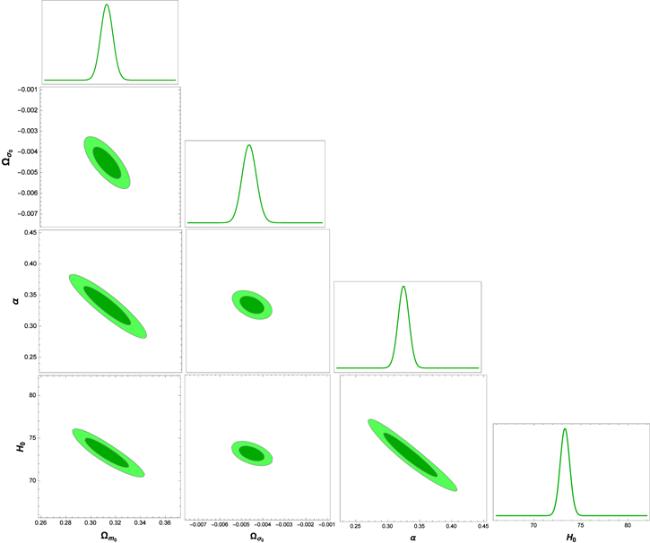
Figure 2. One-dimensional marginalized distribution and two-dimensional contours with 68% CL and 95% CL for RDE in BI model using H(z) data. H0, ${{\rm{\Omega }}}_{{m}_{0}}$, ${{\rm{\Omega }}}_{{\sigma }_{0}}$, α and M are the Hubble parameter, the DM density parameter, the anisotropy parameter, the dimensionless parameter, and the nuisance parameter of SNIa data, respectively. The best-fitted values of these parameters are listed in the third column of table 1. |
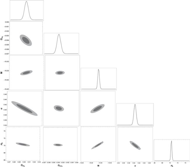
Figure 3. One-dimensional marginalized distribution and two-dimensional contours with 68% CL and 95% CL for RDE in BI model using Pantheon + H(z) data. H0, ${{\rm{\Omega }}}_{{m}_{0}}$, ${{\rm{\Omega }}}_{{\sigma }_{0}}$, α and M are the Hubble parameter, the DM density parameter, the anisotropy parameter, the dimensionless parameter, and the nuisance parameter of SNIa data, respectively. The best-fitted values of these parameters are displayed in the last column of table 1. |
Table 1. 68% CL parameters of RDE in BI model from different observational datasets. |
| Parameters | Pantheon | H(z) | Pantheon + H(z) |
|---|---|---|---|
| ${{\rm{\Omega }}}_{{m}_{0}}$ | 0.259 ± 0.112 | 0.312 ± 0.036 | 0.297 ± 0.031 |
| ${{\rm{\Omega }}}_{{\sigma }_{0}}$ | 0.003 03 ± 0.001 87 | −0.004 53 ± 0.001 09 | −0.004 01 ± 0.001 07 |
| α | 0.436 ± 0.082 | 0.334 ± 0.049 | 0.405 ± 0.033 |
| H0 | 83.251 ± 3.129 | 73.294 ± 1.704 | 70.339 ± 0.743 |
| M | −18.988 ± 0.081 | − | −19.36 ± 0.021 |
| ${\chi }_{\min }^{2}$ | 1006.56 | 22.85 | 1033.37 |
| ${\chi }_{\mathrm{dof}}^{2}$ | 0.965 | 0.476 | 0.944 |
Our joint analysis indicates that the anisotropy parameter change between $5.08\times {10}^{-3}\leqslant {{\rm{\Omega }}}_{{\sigma }_{0}}\leqslant -2.94\times {10}^{-3}$ at 68% error which is 100 times larger than the level of anisotropies, ∼10−3, observed in the CMB measurements. We obtained the constraint ${{\rm{\Omega }}}_{{\sigma }_{0}}\lt {10}^{-3}$ for the joint combination Pantheon + H(z) data. We conclude the approach of our method is compatible with the direct-model independent observational results [46, 53].
In the following, we apply the known Akaike information criterion (AIC) [78] and the Bayesian information criterion (BIC) [79], to examine the quality of the fittings and the relevant observational compatibility of the scenarios. The AIC model selection function can be expressed as [78, 80]
$\begin{eqnarray}{AIC}=-2\mathrm{ln}{{ \mathcal L }}_{\max }+2k+\displaystyle \frac{2k(k+1)}{{N}_{\mathrm{tot}}-k-1},\end{eqnarray}$
with ${{ \mathcal L }}_{\max }$ the maximum likelihood of the datasets, k is the number of parameters of the given model and Ntot the total data points. For a large number of data points Ntot, it reduces to ${AIC}\simeq -2\mathrm{ln}{{ \mathcal L }}_{\max }+2k$. On the other hand, the BIC criterion is an estimator of the Bayesian evidence [79–81], given by $\begin{eqnarray}{BIC}=-2\mathrm{ln}{{ \mathcal L }}_{\max }+k\mathrm{ln}{N}_{\mathrm{tot}}.\end{eqnarray}$
It is obvious that a model consistent with observations should satisfy small AIC and BIC. In [82], the RDE model is investigated with the AIC and BIC criteria and the RDE model is concluded to be ruled out. Reference [83] evaluated ${\chi }_{\min }^{2}$ of ΛCDM model in an anisotropic Universe with Pantheon (Pantheon + H(z)) datasets and found that the ΛCDM in the BI model has a ${\chi }_{\min }^{2}$ of 1012.55 (1039.31). By adopting the AIC and BIC, table 2 also shows that, compared with ΛCDM model, the RDE model in BI Universe is slightly favored by AIC for the joint combination Pantheon + H(z) data. But RDE model is not favored by BIC, though this model has slightly smaller ${\chi }_{\min }^{2}$ than the ΛCDM of the BI model.Table 2. The minimum value of χ2, AIC and BIC of the ΛCDM and Ricci DE models in an anisotropic Universe, by using the Pantheon and Pantheon + H(z) data. |
| Fit | k | ${\chi }_{\min }^{2}$ | AIC | BIC |
|---|---|---|---|---|
| ΛCDM model | ||||
| Pantheon | 4 | 1007.02 | 1015.06 | 1034.84 |
| Pantheon + H(z) | 4 | 1039.31 | 1047.35 | 1067.32 |
| RDE model | ||||
| Pantheon | 5 | 1006.56 | 1016.62 | 1041.33 |
| Pantheon + H(z) | 5 | 1033.37 | 1043.42 | 1068.39 |
5. Physical properties of the RDE of BI Universe
The study of cosmological parameters is an important tool to describe various properties of the Universe. The parameterizations of some functions, alongside some simple numbers, are employed to describe the properties of cosmological parameters. These parameters are describing the global dynamics of the Universe, i.e. the expansion rate and the curvature. We have studied some of the basic parameters such as the Hubble parameter, the EoS parameter and the deceleration parameter of our present RDE model in an anisotropic Universe.
5.1. Hubble parameter
In figure 4, we show the evolution of the Hubble parameter H(z) within a $1\sigma ^{\prime} $ confidence level for our model. We compare the latest 52 points of H(z) dataset [71, 72] with the Pantheon and H(z) data. The solid line in the figures represents the theoretical curve for the best-fit values determined by the joint analysis using Pantheon and H(z) data, which is in good agreement with the observational data.
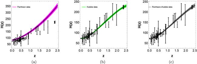
Figure 4. Evolution of the Hubble parameter (in units of km s−1 Mpc−1) with redshift z based on the RDE model in an anisotropy Universe by using the Pantheon (in magenta), H(z) (in green) and Panteon + H(z) (in gray) data. The colored regions show the $1\sigma ^{\prime} $ region, whereas the black dots and bars correspond to the 52 H(z) data points. The cosmological parameters are indicated in of table 1. |
Following equations (13 ) and (21 ), the distance modulus for different redshifts and the evolution of the Hubble parameter for RDE in the BI model are computed by adopting the above mentioned parameter values. Figure 5 illustrates the distance module by taking the best values of the free parameters fixed by Pantheon and H(z) data in an anisotropic Universe. Our results show the predicted μ(z) are similar in three datasets. Moreover, we conclude that at large redshift, the results of the RDE model with both H(z) and Pantheon + H(z) are consistent with the data.
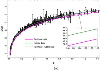
Figure 5. Evolution of the supernova distance modulus with redshift z based on the RDE model in an anisotropy Universe by using the Pantheon (in magenta), H(z) (in green) and Panteon + H(z) (in gray) data. The cosmological parameters are provided in table 1. |
5.2. EoS parameter
Assuming equations (13 ) and (19 ) for the best-fit values, we plot the EoS parameter of RDE in an anisotropic Universe. They are shown in figure 6. It is also observed that the RDE of the BI model does cross the phantom divide line. In other words, in the distant future, the EoS parameter approaches ω < −1, and the Universe evolves into the phantom-dominated epoch. The present values ωde(z = 0) = −1.22, −1.51 and −1.17 can be calculated for the best-fit values of parameters with Pantheon, H(z) and Pantheon + H(z), respectively. These values are comparatively smaller than that predicted by the joint analysis of WMAP + BAO + H(z) + SNIa data which is around −0.93.
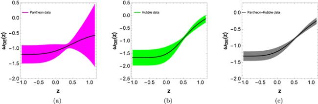
Figure 6. Plots of ωde(z) versus z for the model parameters obtained from bounding the derived model with Pantheon (left panel), H(z) (middle) and Pantheon + H(z) data (right panel). In these plots, the black curves correspond the evolution of ωde(z) for the best-fit case and the colored regions indicate $1\sigma ^{\prime} $ error region. |
5.3. Deceleration parameter
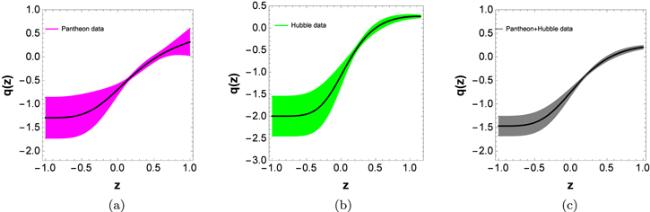
Finally, the best fit curve of q(z) at 68% confidence level is shown in figure 7. Using our anisotropic model, the present value of deceleration parameter are estimated as ${q}_{0}=-{0.686}_{-0.131}^{+0.105}$, ${q}_{0}=-{1.079}_{-0.230}^{+0.234}$ and ${q}_{0}=-{0.749}_{-0.086}^{+0.076}$ fit with Pantheon, H(z) and Pantheon + H(z) data, respectively. It is worthwhile to note that in [84], the authors have obtained q0 = −0.56 ± 0.04 which is bigger than the value of q0, constrained in this work. Therefore, in the proposed model, the results are compatible with recent observations. Moreover, we observe that the early Universe was in a decelerated phase of expansion while the current Universe repels its ingredient RDE of BI model with acceleration. Hence, the Universe with derived model represents a model of a transiting Universe that has signature flipping at ${z}_{\mathrm{tr}}={0.552}_{-0.073}^{+0.105}$, ${z}_{\mathrm{tr}}={0.504}_{-0.069}^{+0.096}$ and ${z}_{\mathrm{tr}}={0.551}_{-0.056}^{+0.074}$ with respect to Pantheon, H(z) and Pantheon + H(z) data, respectively. These transition redshift values are compatible with the recently constrained value ${z}_{\mathrm{tr}}={0.60}_{-0.12}^{+0.21}$ of [85]. From the Pantheon and the combination of H(z) and Pantheon datasets, we note that the transition from deceleration to acceleration in the RDE of the BI expansion process occurs at a redshift of ${z}_{\mathrm{tr}}\sim 0.55$ which is consistent with the results of [86, 87]. So, we observe that in all three cases, our model support the recent scientific findings, as well.
Figure 7. Plots of q(z) versus z for the model parameters obtained from bounding the derived model with Pantheon (left panel), H(z) (middle) and Pantheon + H(z) data (right panel). In these plots, the black curves correspond the evolution of q(z) for the best-fit case and the colored regions indicate $1\sigma ^{\prime} $ error region. |
6. Conclusion
In the present work, we have investigated the BI anisotropic Universe using a well formulated RDE model against the most recent publicly available SNIa compilations. In order to reduce the correlation with background cosmology, we have used the H(z) constraint on the free cosmological parameters. Based on a non-parametric assumption of the kinematic parameters, we reconstructed the Hubble, deceleration and the EoS parameter from a χ2 minimisation technique with 52 data points for observational H(z) values in the redshift range 0 ≤ z ≤ 2.36 which was used to obtain the free parameters of the RDE model in an anisotropic Universe. We also carried out an analysis from the Pantheon compilation data from 1048 SNIa apparent magnitude measurements including 276 SNIa in the low-redshift range 0.3 ≤ z ≤ 0.65. It is interesting to further explore the more intimate connection between the log-marginal likelihood and the ${\chi }_{\min }^{2}$. The main result of the statistical analysis is given in table 1. Thus, we concluded the present Pantheon and H(z) data provides well constrained values of H0 and therefore our model has good consistency with recent observations. The conclusion that 70.3 km s−1 Mpc−1 is close to Planck and not close to previous SNe measurements might be an overstatement, as it sits quite cleanly in the middle. From the joint analysis, it is obtained that the anisotropy parameter of the RDE model changed between $5.08\times {10}^{-3}\leqslant {{\rm{\Omega }}}_{{\sigma }_{0}}\leqslant -2.94\times {10}^{-3}$ at 68% confidence level. This result is not in good agreement with what was obtained from recent CMB observations which indicated the anisotropy parameter is of an order of ∼10−5. In fact, this parameter is important in the study of the early Universe i.e at high redshifts when the anisotropy plays a more effective role in the structure formation of our Universe. From figures 1–3, it has been observed that these best-fit values of the model parameters were well in agreement with the predictions of the RDE model. The reduced ${\chi }_{\mathrm{dof}}^{2}$ obtained for the RDE model fitted extremely well to the considered observational data. In particular, for the Pantheon and H(z) data combination, we confirmed a reasonable and fairly restrictive summary value of ${{\rm{\Omega }}}_{{m}_{0}}=0.297\pm 0.031$ which was in good agreement with many other recent measurements (e.g. 0.315 ± 0.007 from Planck Collaboration [3]).
The study of the evolution of different cosmological parameters like the Hubble parameter, the distance modulus, the EoS of the RDE, and the cosmic deceleration parameter showed that the BI model highly matches observations and followed the standard scenario of the context of the Universe's evolution. Applying best-fit values alongside Pantheon data combined with H(z) data was employed to represent the transition value of the redshift (${z}_{\mathrm{tr}}=0.551$), the current of the deceleration parameter (q0 = −0.749) and the EoS parameter (ωde(z = 0) = −1.17) in the RDE of BI model. Finally, the behavior of the model was in good agreement with the modern cosmological observations. In the absence of anisotropy effects, i.e. σ0 = 0, and ${{\rm{\Omega }}}_{{\sigma }_{0}}=0$ (i.e. spatially flat FRW Universe), the RDE is reduced to that of [17, 20, 32, 88, 89]. Comparing the results obtained in the RED model of FRW in [17, 20, 32, 88, 89], it was observed that the presence of anisotropy effects leads improves the data fitting in the RDE model.