Welcome to visit Communications in Theoretical Physics,
Gravitation Theory, Astrophysics and Cosmology

Quasinormal modes and absorption of a massless scalar field for the magnetic Gauss–Bonnet black hole

  • Chen Ma ,
  • Yu Zhang ,
  • Qian Li ,
  • Zhi-Wen Lin
Expand
  • Faculty of Science, Kunming University of Science and Technology, Kunming, Yunnan 650500, China

Received date: 2022-03-13

  Revised date: 2022-04-04

  Accepted date: 2022-04-27

  Online published: 2022-06-09

Copyright

© 2022 Institute of Theoretical Physics CAS, Chinese Physical Society and IOP Publishing

Abstract

We study the massless scalar quasinormal frequencies of an asymptotically flat static and spherically symmetric black hole with a nonzero magnetic charge in four-dimensional extended scalar-tensor-Gauss–Bonnet theory. The results show that the real part of the quasinormal frequency becomes larger and the imaginary part becomes smaller with increasing the magnetic charge or the angular harmonic index. The existence of magnetic charges will reduce the damping of scalar perturbation, but increase the frequency. We also study the absorption cross-section of the scalar field in this black hole. We find that its curve will become lower as the magnetic charge increases, i.e. the magnetic charge will weaken the absorption capacity of the black hole. Meanwhile, the high-frequency limit of the total absorption cross-section is just the area of black hole shadow.

Cite this article

Chen Ma , Yu Zhang , Qian Li , Zhi-Wen Lin . Quasinormal modes and absorption of a massless scalar field for the magnetic Gauss–Bonnet black hole[J]. Communications in Theoretical Physics, 2022 , 74(6) : 065402 . DOI: 10.1088/1572-9494/ac6ac2

1. Introduction

Due to the discovery of gravitational waves, the existence of black holes has become a reality [13]. The quasinormal modes (QNMs) are called the characteristic sound of black holes, which are of great significance to the exploration of black holes. It is well known that QNMs satisfy the appropriate boundary conditions, that is, the waves must be purely ingoing at the event horizon and purely outgoing at infinity. They have discrete complex frequency values, in which the real part represents the frequency of the oscillation, and the imaginary part represents the attenuation of the oscillation [4]. In order to better understand the kinetic of black holes, more and more researchers have studied the QNMs, and got very meaningful results. The scalar perturbation [4, 5], the electromagnetic perturbation [6, 7], the Dirac perturbation [8] and the gravitational perturbation [9], have all been discussed. Moreover, in AdS/CFT theory, one can obtain the thermalization timescale by calculating the quasinormal frequency [10].
Another important issue is the wave scattering problem of black holes. Scattering by gravitational sources has been an important test for General Relativity. In previous works, Dolan et al studied the Fermion scattering by Schwarzschild black hole [11]. Crispino and Oliveira studied the electromagnetic absorption by Reissner–Nordström black hole [12]. Benone et al studied the absorption of a massive scalar field by a charged black hole [13]. Chakrabarty studied the absorption of a black hole surrounded by quintessence [5]. Considering that there is a potential barrier outside the black hole, the waves emitted to the black hole (or emitted by the black hole) will be reflected and transmitted. Through the analysis of the scattered wave, the observer at infinity can receive the information sent by the black hole and infer the internal structure of the black hole.
On the other hand, General Relativity requires the dynamics are two-derivative systems, which is probably the weakest link in it. Many researchers consider higher-derivative extensions to Einstein gravity, and one of the relatively successful attempts is the Gauss–Bonnet gravity theory. If the scalar field is coupled with the Gauss–Bonnet invariant, the extended scalar-tensor-Gauss–Bonnet (ESTGB) theory can be obtained [14]. In [15], the authors firstly found the exact asymptotically flat static and spherically symmetric black hole solution for the four-dimensional extended scalar-tensor-Gauss–Bonnet theory coupled to the nonlinear electrodynamics. The nonlinear electrodynamics will reduce to Maxwell's theory in the weak field limit and satisfy the weak energy condition.
We know that for pure Gauss–Bonnet gravity, the Gauss–Bonnet term is just a topological term, and the Gauss–Bonnet AdS black hole degenerates into a four-dimensional normal AdS black hole. Hence for the Gauss–Bonnet AdS black hole, the spacetime is at least four-dimensional. While for extended scalar-tensor-Gauss–Bonnet theory, we have an asymptotically flat static and spherically symmetric black hole solution in four-dimensions. The black hole itself has very important research value, and it has a nonzero magnetic charge and scalar hair, which turns out to be dependent on the magnetic charge. Based on this, we take the black hole as the background to discuss and analyze its dynamic behavior. We use the 6th order WKB approximation to calculate the quasinormal frequencies and the absorption cross section of a massless scalar field in the magnetic Gauss–Bonnet black hole spacetime and point out the specific influence of black hole parameters on it.
In section 2, we review the magnetic Gauss–Bonnet black hole solution and study the massless free scalar field equation. In section 3, we calculate the quasinormal frequencies of the magnetic Gauss–Bonnet black hole. In section 4, we calculate the gray-body factor and absorption cross-section and give the corresponding analysis. Conclusions are presented in section 5.

2. The background spacetime and free scalar field dynamics

The black hole solution with nontrivial scalar hair can be obtained by directly coupling the scalar field with the second-order algebraic curvature invariants. In particular, the ESTGB theory considers the coupling of the scalar field with Gauss–Bonnet invariant, and the scalar hair is maintained by interacting with the curvature of spacetime [14]. The action of the four-dimensional ESTGB theory with matter field is defined by [15]
$\begin{eqnarray}\begin{array}{rcl}S & = & \displaystyle \int {{\rm{d}}}^{4}x\sqrt{-g}\left\{\displaystyle \frac{1}{16\pi }\left(R-\displaystyle \frac{1}{2}{\partial }_{\mu }\phi {\partial }^{\mu }\phi \right.\right.\\ & & \left.\left.+f\left(\phi \right){R}_{\mathrm{GB}}^{2}-2U\left(\phi \right)\right)-\displaystyle \frac{1}{4\pi }{{ \mathcal L }}_{\mathrm{matter}}\right\},\end{array}\end{eqnarray}$
where the Gauss–Bonnet term is non-minimally coupled to the scalar field by $f\left(\phi \right)$ and $U\left(\phi \right)$, which are the function and potential of the scalar field, respectively. They are given by
$\begin{eqnarray}\begin{array}{rcl}f\left(\phi \right) & = & -\displaystyle \frac{{{\ell }}^{2}\sigma }{32}\left\{\sqrt{2\sigma }{\tan }^{{}^{-1}}\left(\displaystyle \frac{\sqrt{2}}{\sqrt{\sigma }\quad \phi }\right)\right.\\ & & \left.+\displaystyle \frac{1}{2\phi }\mathrm{ln}\left[{\left(\displaystyle \frac{2\beta }{\sigma {\phi }^{2}}+\beta \right)}^{2}\right]-\displaystyle \frac{2}{\phi }\right\},\end{array}\end{eqnarray}$
$\begin{eqnarray}\begin{array}{rcl}U\left(\phi \right) & = & \displaystyle \frac{{2}^{{}^{\tfrac{9}{2}}}}{105{{\ell }}^{2}{\sigma }^{{}^{\tfrac{7}{2}}}}\left[\displaystyle \frac{\pi }{2}-{\tan }^{{}^{-1}}\left(\displaystyle \frac{\sqrt{2}}{\sqrt{\sigma }\phi }\right)\right]\\ & & +\displaystyle \frac{{\phi }^{5}}{4{{\ell }}^{2}}\left(\displaystyle \frac{3}{10\sigma }+\displaystyle \frac{5{\phi }^{2}}{7}+\displaystyle \frac{7\sigma {\phi }^{4}}{24}\right)\mathrm{ln}\left[{\left(\displaystyle \frac{2\beta }{\sigma {\phi }^{2}}+\beta \right)}^{2}\right]\\ & & -\displaystyle \frac{\phi }{3{{\ell }}^{2}}\left(\displaystyle \frac{16}{35{\sigma }^{3}}-\displaystyle \frac{8{\phi }^{2}}{105{\sigma }^{2}}+\displaystyle \frac{31{\phi }^{4}}{70\sigma }+\displaystyle \frac{11{\phi }^{6}}{28}\right).\end{array}\end{eqnarray}$
And the NLED Lagrangian in the weak-field limit is given by
$\begin{eqnarray}\begin{array}{rcl}{{ \mathcal L }}_{\mathrm{NLED}} & = & \displaystyle \frac{{ \mathcal F }}{8}-{s}^{{}^{\tfrac{1}{2}}}\left(1+\displaystyle \frac{37}{210{\sigma }_{* }}+\displaystyle \frac{2}{525{\sigma }_{* }}\right){{ \mathcal F }}^{{}^{\tfrac{5}{4}}}\\ & & -\displaystyle \frac{{\sigma }_{* }s{{ \mathcal F }}^{{}^{\tfrac{3}{2}}}}{16}+{ \mathcal O }({{ \mathcal F }}^{{}^{\tfrac{7}{4}}}),\end{array}\end{eqnarray}$
where the electromagnetic field invariant ${ \mathcal F }={q}^{2}/{r}^{4}$.
When the parameters satisfy the relations
$\begin{eqnarray}\begin{array}{rcl}\sigma & = & {\sigma }_{* }=\displaystyle \frac{q}{m},\quad \quad \quad {\ell }=s=q,\\ \beta & = & {\beta }_{* },\end{array}\end{eqnarray}$
the asymptotically flat static and spherically symmetric black hole solution is given by
$\begin{eqnarray}\begin{array}{rcl}{\rm{d}}{s}^{2} & = & -f(r){\rm{d}}{t}^{2}+f{\left(r\right)}^{-1}{\rm{d}}{r}^{2}\\ & & +{r}^{2}\left({\rm{d}}{\theta }^{2}+{\sin }^{2}\theta {\rm{d}}{\phi }^{2}\right),\end{array}\end{eqnarray}$
where
$\begin{eqnarray}f(r)=1-\displaystyle \frac{2m}{r}-\displaystyle \frac{{q}^{3}}{{r}^{3}}.\end{eqnarray}$
Here q is the magnetic charge, and the scalar field is
$\begin{eqnarray}\phi (r)=\displaystyle \frac{q}{r}.\end{eqnarray}$
Due to the scalar charge being proportional to the magnetic charge, the scalar hair is not accompanied by any new information for the black hole, therefore this scalar hair constitutes the second type of legal hair. In the case q = 0, it represents the Schwarzscild black hole, and in the case m = 0, we can obtain a purely magnetic Gauss–Bonnet black hole. By requiring the weak energy condition to be satisfied, only values of q < 0 are allowed. Moreover, in order to keep our research object as a non-extreme black hole, q/m > − 1.058 must be satisfied.
The dynamics of a massless free scalar field in the black hole background spacetime (6) is given by the Klien–Gordon equation
$\begin{eqnarray}{{\rm{\nabla }}}_{\mu }{{\rm{\nabla }}}^{\mu }{\rm{\Phi }}=0.\end{eqnarray}$
We emphasize that this free scalar field is different from the coupled scalar field. In order to separate the variables, we use the ansatz
$\begin{eqnarray}{{\rm{\Phi }}}_{\omega l}(t,r,\theta ,\phi )=\displaystyle \frac{{\psi }_{\omega l}(r)}{r}{Y}_{l}^{m}(\theta ,\phi ){{\rm{e}}}^{-{\rm{i}}\omega t},\end{eqnarray}$
where ${Y}_{l}^{m}(\theta ,\phi )$ are the spherical harmonics.
The tortoise coordinate r* is defined as
$\begin{eqnarray}{\rm{d}}{r}_{* }=\displaystyle \frac{{\rm{d}}r}{f(r)},\end{eqnarray}$
substituting equations (6), (10) and (11) into equation (9), we can obtain the radial scalar field equation
$\begin{eqnarray}\displaystyle \frac{{{\rm{d}}}^{2}\psi }{{\rm{d}}{r}_{* }^{2}}+({\omega }^{2}-V(r))\psi =0,\end{eqnarray}$
where
$\begin{eqnarray}V(r)=f(r)\left(\displaystyle \frac{f^{\prime} (r)}{r}+\displaystyle \frac{l(l+1)}{{r}^{2}}\right).\end{eqnarray}$
The effective potential V(r) is dependent on the black hole mass m, the magnetic charge q, and the angular harmonic index l. We plot the behavior of the effective potential for the different values of q and l in figure 1. We can find that the peak of the effective potential moves to the left and becomes higher as the absolute value of q increases for fixed l in figure 1(a); and the peak of the effective potential moves to the right and becomes higher as l increases for fixed q in figure 1(b).
Figure 1. Behavior of the effective potential V(r). (a) Behavior of the effective potential V (r) with l = 3, q = −0.4, −0.8, −1.0. (b) Behavior of the effective potential V (r) with q = −0.4, l = 1, 2, 3.

3. The quasinormal modes

QNMs are the solutions of the Schrödinger-like equation (12). We impose the requirement that QNMs have appropriate boundary conditions, that is, the waves are purely ingoing at the horizon and purely outgoing at infinity:
$\begin{eqnarray}\psi \sim \left\{\begin{array}{ll}{{\rm{e}}}^{-{\rm{i}}\omega {r}_{* }}, & \mathrm{as}\qquad {r}_{* }\to -\infty ,\\ {{\rm{e}}}^{{\rm{i}}\omega {r}_{* }}, & \mathrm{as}\qquad {r}_{* }\to +\infty .\end{array}\right.\end{eqnarray}$
In this paper, we use the WKB method for our calculation. The WKB method approximation for calculating the quasinormal modes of a black hole was first proposed by Schutz and Will [16] in 1985. In 1987, the 3rd order extension for this approach was developed by Iyer and Will [17]. In 2003, the method was extended to the 6th order by Konoplya [18]. In 2017, Matyjasek and Opala [19] developed the approach to the 13th order.
The result of the 3rd order WKB method [17] for QNMs is as follows
$\begin{eqnarray}\begin{array}{rcl}{\omega }^{2} & = & ({V}_{0}+\sqrt{-2{V}_{0}^{{\prime\prime} }}{\rm{\Lambda }})\\ & & -{\rm{i}}(n+\displaystyle \frac{1}{2})\displaystyle \frac{1}{\sqrt{-2{V}_{0}^{{\prime\prime} }}}(1+{\rm{\Omega }}),\end{array}\end{eqnarray}$
where
$\begin{eqnarray}\begin{array}{rcl}{\rm{\Lambda }} & = & \displaystyle \frac{1}{\sqrt{-2{V}_{0}^{{\prime\prime} }}}\left(\displaystyle \frac{1}{8}\left(\displaystyle \frac{{V}_{0}^{(4)}}{{V}_{0}^{{\prime\prime} }}\right)\left({\alpha }^{2}+\displaystyle \frac{1}{4}\right)\right.\\ & & \left.-\displaystyle \frac{1}{288}\left({\left(\displaystyle \frac{{V}_{0}^{(3)}}{{V}_{0}^{{\prime\prime} }}\right)}^{2}(60{\alpha }^{2}+7)\right)\right),\end{array}\end{eqnarray}$
$\begin{eqnarray}\begin{array}{rcl}{\rm{\Omega }} & = & \displaystyle \frac{1}{-2{V}_{0}^{{\rm{{\prime} }}{\rm{{\prime} }}}}\left(\displaystyle \frac{5}{6912}{\left(\displaystyle \frac{{V}_{0}^{(3)}}{{V}_{0}^{{\rm{{\prime} }}{\rm{{\prime} }}}}\right)}^{4}(188{\alpha }^{2}+77)\right.\\ & & -\displaystyle \frac{1}{384}\left(\displaystyle \frac{{V}_{0}^{(3)2}{V}_{0}^{(4)}}{{V}_{0}^{{\rm{{\prime} }}{\rm{{\prime} }}3}}\right)(100{\alpha }^{2}+51)\\ & & +\displaystyle \frac{1}{2304}{\left(\displaystyle \frac{{V}_{0}^{(4)}}{{V}_{0}^{{\rm{{\prime} }}{\rm{{\prime} }}}}\right)}^{2}(68{\alpha }^{2}+67)\\ & & +\displaystyle \frac{1}{288}\left(\displaystyle \frac{{V}_{0}^{{\rm{{\prime} }}{\rm{{\prime} }}{\rm{{\prime} }}}{V}_{0}^{(5)}}{{V}_{0}^{{\rm{{\prime} }}{\rm{{\prime} }}2}}\right)(28{\alpha }^{2}+19)\\ & & \left.-\displaystyle \frac{1}{288}\left(\displaystyle \frac{{V}_{0}^{(6)}}{{V}_{0}^{{\rm{{\prime} }}{\rm{{\prime} }}}}\right)(4{\alpha }^{2}+5)\right),\end{array}\end{eqnarray}$
and
$\begin{eqnarray}\alpha =n{\left.+\displaystyle \frac{1}{2},\qquad {V}_{0}^{(n)}=\displaystyle \frac{{{\rm{d}}}^{n}V}{{\rm{d}}{r}_{* }^{n}}\right|}_{{r}_{* }={r}_{* }({r}_{p})}.\end{eqnarray}$
The form of the result of the 6th order WKB method [18] for QNMs is as follows
$\begin{eqnarray}\displaystyle \frac{{\rm{i}}({\omega }^{2}-{V}_{0})}{\sqrt{-2{V}_{0}^{{\prime\prime} }}}+\sum _{j=2}^{6}{{\rm{\Lambda }}}_{j}=n+\displaystyle \frac{1}{2},\end{eqnarray}$
where Λj are presented in [18].
We list the results of the 6th order WKB method for QNMs in table 1, where l is the angular harmonic index, n is the overtone number, and q is the magnetic charge.
Table 1. The QNMs of the magnetic Gauss–Bonnet black hole with q = −0.2, −0.4, −0.6, −0.8, −1.0.
l n ω (q = −0.2) ω (q = −0.4) ω (q = −0.6) ω (q = −0.8) ω (q = −1.0)
1 0 0.293048 − 0.0977316i 0.294029 − 0.0975119i 0.296807 − 0.0968192i 0.302764 − 0.0949061i 0.314077 − 0.0886489i
1 0.264667 − 0.306401i 0.266057 − 0.305544i 0.269962 − 0.302871i 0.278002 − 0.295519i 0.287643 − 0.273043i

2 0 0.483862 − 0.0967364i 0.485422 − 0.0965197i 0.489844 − 0.0958430i 0.499358 − 0.0940295i 0.518478 − 0.0882874i
1 0.464106 − 0.295527i 0.465941 − 0.294800i 0.471125 − 0.292536i 0.482099 − 0.286495i 0.501498 − 0.267776i
2 0.430712 − 0.508500i 0.433016 − 0.507043i 0.439467 − 0.502535i 0.452653 − 0.490619i 0.469698 − 0.455538i

3 0 0.675670 − 0.0964713i 0.677826 − 0.0962576i 0.683939 − 0.0955913i 0.697129 − 0.0938113i 0.724068 − 0.0881808i
1 0.661004 − 0.292194i 0.663362 − 0.291513i 0.670037 − 0.289392i 0.684316 − 0.283740i 0.711697 − 0.266068i
2 0.633977 − 0.495836i 0.636710 − 0.494567i 0.644414 − 0.490631i 0.660609 − 0.480204i 0.687788 − 0.448399i
3 0.598885 − 0.711104i 0.602106 − 0.709064i 0.611124 − 0.702763i 0.629563 − 0.686209i 0.653874 − 0.637709i
We plot the quasinormal frequencies of scalar field with respect to the spherical harmonic index l for q = − 0.4, − 0.8, − 1.0 in figures 2 and 3 for n = 0, 1, respectively. Figures 2(a) and 3(a) panels show the real part of the quasinormal frequency and figures 2(b) and 3(b) panels show the imaginary part of the frequency.
Figure 2. The quasinormal frequencies with n = 0. (a) The real part of quasinormal frequencies with n = 0, q = −0.4, −0.8, −1.0. (b) The imaginary part of quasinormal frequencies with n = 0, q = −0.4, −0.8, −1.0.
From table 1 (or figures 2 and 3), we can see that for the fixed parameters l and n, the real part of quasinormal frequency increases and the imaginary part decreases with the increase of the absolute value of magnetic charge ∣q∣. The real and imaginary parts of the quasinormal frequency correspond to the actual frequency and decay rate of the perturbation field, respectively. This means that as the magnetic charge ∣q∣ increases, the actual frequency of the scalar perturbation around the black hole increases, but the decay becomes slower. In other words, the presence of a magnetic charge will reduce the damping of the scalar perturbation, but the oscillation frequency will be higher. When q and n remain unchanged, with the increase of spherical harmonic index l, the real part of the quasinormal frequency increases almost linearly, and the imaginary part slightly decreases. When q and l are unchanged, with the increase of the overtone index n, the real part of the quasinormal frequency decreases, and the imaginary part increases. This means that the higher modal phase of the QNM decays faster than the lower modal so that the fundamental quasi-normal frequencies n = 0 dominate.
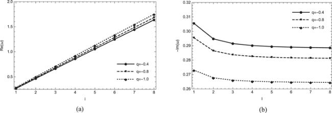
Figure 3. The quasinormal frequencies with n = 1. (a) The real part of quasinormal frequencies with n = 1, q = −0.4, −0.8, −1.0. (b) The imaginary part of quasinormal frequencies with n = 1, q = −0.4, −0.8, −1.0.

4. Gray-body factors and absorption cross-section

Hawking emission spectrum is not a perfect black body spectrum to an asymptotic observer, and the deviation of the Hawking radiation spectrum from the exact black body spectrum can be described by the gray-body factor [20]. In this section, we discuss the gray-body factors and absorption cross-section for the massless scalar field of the magnetic Gauss–Bonnet black hole. We will use the 6th order WKB method for our calculation.

4.1. Gray-body factors

We consider the asymptotic solution of equation (12). Since we are interested in the absorption process, we set the boundary conditions as
$\begin{eqnarray}\psi \sim \left\{\begin{array}{ll}T(\omega ){{\rm{e}}}^{-{\rm{i}}\omega {r}_{* }}, & \mathrm{as}\qquad {r}_{* }\to -\infty ,\\ {{\rm{e}}}^{-{\rm{i}}\omega {r}_{* }}+R(\omega ){{\rm{e}}}^{{\rm{i}}\omega {r}_{* }}, & \mathrm{as}\qquad {r}_{* }\to +\infty ,\end{array}\right.\end{eqnarray}$
where T(ω) and R(ω) are the transmission and reflection coefficient, and due to conservation of flux, they satisfy
$\begin{eqnarray}{\left|T(\omega )\right|}^{2}+{\left|R(\omega )\right|}^{2}=1.\end{eqnarray}$
The gray-body factor γ(ω) is defined as the square of the absolute value of the transmission coefficient ${\left|T(\omega )\right|}^{2}$.
In the WKB approximation, the reflection coefficient is defined as
$\begin{eqnarray}R{(\omega )=(1+{{\rm{e}}}^{-2\pi {\rm{i}}\alpha })}^{-\displaystyle \frac{1}{2}}.\end{eqnarray}$
We plot the dependence of ${\left|T(\omega )\right|}^{2}$ and ${\left|R(\omega )\right|}^{2}$ on ω for different spherical harmonic indices l and magnetic charges q in figures 4 and 5, respectively. As can be seen from figures 4 and 5, the transmission coefficient ${\left|T(\omega )\right|}^{2}$, or gray-body factor γ(ω), tends to be 1 at higher frequencies and tends to be 0 at lower frequencies. This means that the higher-frequency waves are more likely to be absorbed by black holes. Similarly, the lower-frequency waves are more likely to be scattered by black holes. The presence of magnetic charge reduces the gray-body factor, which makes it harder for waves of the same frequency to be absorbed by the black hole.
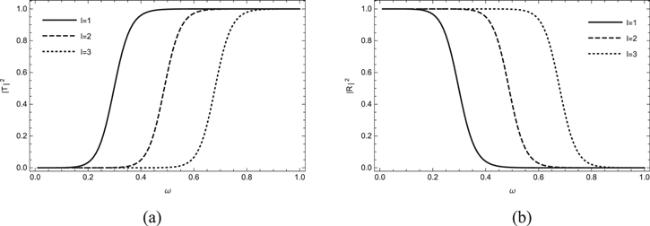
Figure 4. The dependence of ${\left|T(\omega )\right|}^{2}$ and ${\left|R(\omega )\right|}^{2}$ on ω for different spherical harmonic indices l with q = − 0.4. (a) The dependence of ∣T(ω)∣2 on ω for different spherical harmonic indices l. (b) The dependence of ∣R(ω)∣2 on ω for different spherical harmonic indices l.
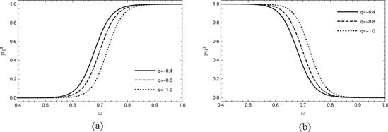
Figure 5. The dependence of ${\left|T(\omega )\right|}^{2}$ and ${\left|R(\omega )\right|}^{2}$ on ω for different magnetic charges q with l = 3. (a) The dependence of ∣T(ω)∣2 on ω for different magnetic charges q. (b) The dependence of ∣R(ω)∣2 on ω for different magnetic charges q.

4.2. Absorption cross section

4.2.1. Numerical computations

Partial and total absorption cross-sections are defined as
$\begin{eqnarray}{\sigma }_{l}=\displaystyle \frac{\pi (2l+1)}{{\omega }^{2}}{\left|T(\omega )\right|}^{2},\end{eqnarray}$
$\begin{eqnarray}\sigma =\sum _{l=0}^{\infty }{\sigma }_{l}.\end{eqnarray}$
We plot the variation of partial absorption cross-section σl for different spherical harmonic indices l and magnetic charges q in figure 6. Figure 6(a) shows the variation of partial absorption cross-section σl for different spherical harmonic indices l , and figure 6(b) shows the dependence of σl on ω for different magnetic charges q.
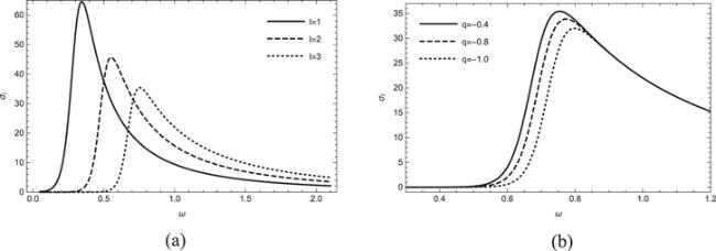
Figure 6. The dependence of σl on ω for different magnetic charges q and spherical harmonic indices l. (a) The dependence of σl on ω for different spherical harmonic indices l with q = −0.4. (b) The dependence of σl on ω for different magnetic charges q with l = 3.
It can be seen from figure 6 that the partial absorption cross-section has a peak, and the position of the peak shifts to the right as l or ∣q∣ increases, while the peak decreases. This shows that for a fixed spherical harmonic index, black holes are more likely to absorb waves in a certain frequency band, and the frequency band increases with the increase of l. The existence of the magnetic charge q will shift the frequency band corresponding to each l to the right as a whole.
We also plot the total absorption cross-section σ with respect to the frequency ω for q = − 0.4, − 0.8, − 1.0 in figure 7, and for convenience we calculated the sum of the modes from l = 0 to l = 10 to approximate σ.
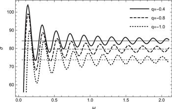
Figure 7. The dependence of σ on ω (black lines) and the high-frequency limit of the absorption cross-section σhf (gray lines) for different magnetic charges q.

4.2.2. High-frequency limit

As the frequency gets higher and higher, the particle property of the wave function becomes more and more obvious. When the frequency tends to infinity, the wavefront of the massless scalar field propagates along the null geodesics [21]. In this subsection, we analyze the null geodesics in the magnetic Gauss–Bonnet black hole. Without loss of generality, we only consider the motion for a massless particle in the θ = π/2 plane. Through Killing vector fields ∂t and ∂φ, we can get two conserved quantities: energy E and angular momentum L, which are defined as
$\begin{eqnarray}E=f(r)\displaystyle \frac{{\rm{d}}t}{{\rm{d}}\lambda },\end{eqnarray}$
$\begin{eqnarray}L={r}^{2}\displaystyle \frac{{\rm{d}}\phi }{{\rm{d}}\lambda },\end{eqnarray}$
respectively, where λ is the affine parameter.
Substituting equations (25) and (26) into the following equation
$\begin{eqnarray}{g}_{\mu \nu }\displaystyle \frac{{\rm{d}}{x}^{\mu }}{{\rm{d}}\lambda }\displaystyle \frac{{\rm{d}}{x}^{\nu }}{{\rm{d}}\lambda }=0,\end{eqnarray}$
we have
$\begin{eqnarray}T(r)+f(r)\displaystyle \frac{{L}^{2}}{{r}^{2}}={E}^{2},\end{eqnarray}$
where $T(r)\equiv {\left({\rm{d}}r/{\rm{d}}\lambda \right)}^{2}$ is the effective kinetic energy.
There are three different finial states of motion for a massless particle shot at the black hole from infinity. In case (1): the particle will reach the perihelion and then be reflected to infinity; in case (2): the particle orbit will be asymptotically close to the photon sphere; in case (3): the particle will fall into the black hole. Case (2) is the dividing point between cases (1) and (3).
We define the impact parameter bL/E and introduce the function
$\begin{eqnarray}{ \mathcal T }(r,b)=\displaystyle \frac{T(r)}{{L}^{2}}=\displaystyle \frac{1}{{b}^{2}}-\displaystyle \frac{f(r)}{{r}^{2}},\end{eqnarray}$
the particle in case (2) must fulfill two conditions: (I) the effective kinetic energy is 0, i.e. ${ \mathcal T }({r}_{\mathrm{ps}},{b}_{c})=0$, which indicates that there is a perihelion; (II) the time derivative of the effective kinetic energy is 0, i.e. ${\partial }_{t}{ \mathcal T }({r}_{\mathrm{ps}},{b}_{c})=0$, which indicates that the perihelion cannot be reached (Because the angular momentum L is a conserved quantity). We can get the solution (rps, bc) of the equations of conditions (I) and (II). Thus, the high-frequency limit of the absorption cross-section is σhf = πb2, and its physical meaning is the area of black hole shadow.
Based on this analysis, as the frequency increases, the absorption cross-section σ will oscillate around σhf smaller and smaller. We also plot the high-frequency limit of the absorption cross-section σhf in figure 7 using the gray lines, the result of the figure meets our expectations.

5. Conclusions

In this paper, we have used the 6th order WKB approximation to calculate the quasinormal frequencies and the absorption cross-section of a massless scalar field in the magnetic Gauss–Bonnet black hole spacetime.
For the quasinormal frequencies, we have found

As the absolute value of the magnetic charge ∣q∣ increases, the real part of quasinormal frequency increases while its imaginary part decreases. The existence of magnetic charges will reduce the damping of scalar perturbation, but increase the frequency.

As the spherical harmonic index l increases, the real part of quasinormal frequency increases almost linearly, while its imaginary part decreases. Although the decay rate of scalar perturbation decreases, its variation range is very small.

As the overtone index n increases, the real part of quasinormal frequency decreases slightly while its imaginary part increases significantly. The higher the overtone index, the faster the decay. Therefore, the frequency of n = 0 after a certain time is dominant.

For the transmission and reflection coefficients, we have obtained

The transmission coefficient ${\left|T(\omega )\right|}^{2}$ decreases and hence reflection coefficient ${\left|R(\omega )\right|}^{2}$ increases with an increase in spherical harmonic index l or absolute value of the magnetic charge ∣q∣. The existence of a magnetic charge will reduce the gray-body factor, which makes the waves with the same frequency more difficult to be absorbed by the black hole.

In the low-frequency case, the transmission coefficient ${\left|T(\omega )\right|}^{2}\to 0$ and the reflection coefficient ${\left|R(\omega )\right|}^{2}\to 1$. In the high-frequency case, the situation is just the other way round. We have seen that higher frequency waves are more easily absorbed by black holes, and lower frequency waves are more easily scattered by black holes.

For the absorption cross-section, we have found

The peak of the partial absorption cross-sections moves to the right and becomes lower as l or the absolute value of q increases. In other words, the partial wave is more easily scattered by the black hole as the absolute value of the magnetic charge is larger.

The curve of the total absorption cross-section becomes lower as the absolute value of q increases, and its high-frequency limit is the area of black hole shadow. The overall absorption cross-section of the black hole vibrates near its optical geometric limit, that is, the shadow area of the black hole, and converges here. At the same time, the magnetic charge q will weaken the absorption capacity of the black hole.

In the future, we also hope to discuss the electromagnetic perturbation, the Dirac perturbation, and the gravitational perturbation in the background of a four-dimensional extended scalar-tensor-Gauss–Bonnet black hole, so as to obtain more important information about the black hole.

This work was supported partly by the National Natural Science Foundation of China (Grant No. 12065012), Yunnan High-level Talent Training Support Plan Young & Elite Talents Project (Grant No. YNWR-QNBJ-2018-360) and the Fund for Reserve Talents of Young and Middle-aged Academic and Technical Leaders of Yunnan Province (Grant No. 2018HB006).

1
Abbott B P 2016 Observation of gravitational waves from a binary black hole merger Phys. Rev. Lett. 116 061102

DOI

2
Abbott B P 2016 Gw151226: observation of gravitational waves from a 22-solar-mass binary black hole coalescence Phys. Rev. Lett. 116 241103

DOI

3
LIGO Scientific Virgo Collaboration Abbott B P 2018 Erratum: Gw170104: Observation of a 50-solar-mass binary black hole coalescence at redshift 0.2 Phys. Rev. Lett. 121 129901 [phys. rev. lett. 118, 221 101 (2017)]

DOI

4
Zhang Y Li E-K Geng J-L 2014 Quasinormal modes of massless scalar field perturbation of a Reissner–Nordström de sitter black hole with a global monopole Gen. Relativ. Gravitation 46 1 11

DOI

5
Chakrabarty H Abdujabbarov A Bambi C 2019 Scalar perturbations and quasi-normal modes of a nonlinear magnetic-charged black hole surrounded by quintessence Eur. Phys. J. C 79 1 11

DOI

6
Zhang Y Gui Y-X Yu F Li F-L 2007 Quasinormal modes of a schwarzschild black hole surrounded by free static spherically symmetric quintessence: electromagnetic perturbations Gen. Relativ. Gravitation 39 1003 1010

DOI

7
Zhang Y Gui Y-X Yu F Wang F-J 2007 Quasinormal modes of electromagnetic perturbation around a stringy black hole Chin. Phys. Lett. 24 2749

DOI

8
Zhang Y Wang C-Y Gui Y-X Wang F-J Yu F 2009 Dirac quasinormal modes of a schwarzschild black hole surrounded by free static spherically symmetric quintessence Chin. Phys. Lett. 26 030401

DOI

9
Zhang Y Gui Y-X 2006 Quasinormal modes of gravitational perturbation around a schwarzschild black hole surrounded by quintessence Classical Quantum Gravity 23 6141

DOI

10
Cardoso V 2004 Quasinormal modes and gravitational radiation in black hole spacetimes arXiv: gr-qc/0404093

11
Dolan S Doran C Lasenby A 2006 Fermion scattering by a schwarzschild black hole Phys. Rev. D 74 064005

DOI

12
Crispino L C B Oliveira E S 2008 Electromagnetic absorption cross section of Reissner–Nordström black holes Phys. Rev. D 78 024011

DOI

13
Benone C L de Oliveira E S Dolan S R Crispino L C B 2014 Absorption of a massive scalar field by a charged black hole Phys. Rev. D 89 104053

DOI

14
Doneva D D Kiorpelidi S Nedkova P G Papantonopoulos E Yazadjiev S S 2018 Charged Gauss–Bonnet black holes with curvature induced scalarization in the extended scalar-tensor theories Phys. Rev. D 98 104056

DOI

15
Cañate P Bergliaffa S E P 2020 Novel exact magnetic black hole solution in four-dimensional extended scalar-tensor-Gauss–Bonnet theory Phys. Rev. D 102 104038

DOI

16
Schutz B F Will C M 1985 Black hole normal modes: a semianalytic approach Astrophys. J. 291 L33 L36

DOI

17
Iyer S Will C M 1987 Black-hole normal modes: a wkb approach. i. foundations and application of a higher-order wkb analysis of potential-barrier scattering Phys. Rev. D 35 3621

DOI

18
Konoplya R A 2003 Quasinormal behavior of the d-dimensional schwarzschild black hole and the higher order wkb approach Phys. Rev. D 68 024018

DOI

19
Matyjasek J Opala M 2017 Quasinormal modes of black holes: the improved semianalytic approach Phys. Rev. D 96 024011

DOI

20
Chowdhury A 2021 On the effect of scalar fields on hawking radiation and quasinormal modes of black holes arXiv:2106.02294

21
Li P Huang Y Li X-Z 2021 Absorption of massless scalar field by furry black holes in de rham-gabadadze-tolley theory arXiv:2102.12102

Outlines

/