


1. Introduction
Recently, the optical properties of semiconductor nanostructures have attracted a lot of interest in the field of theory and application, since the enhanced nonlinear optical effects have been found in the low-dimensional quantum systems in comparison with bulk materials [1–4]. Owing to the development of advanced materials growing technology, the different quantum confined systems based on semiconductor nanostructures can be fabricated, which can promote the wide application in electronic and optoelectronic devices [5, 6]. Much attention has been focused on semiconductor quantum well (QW), quantum wire, and quantum dot, which can make the performance of the devices improved significantly in comparison with the conventional technology. Among the low-dimensional semiconductor nanostructures, the semiconductor QWs with larger band gaps are easier to grow and convenient to be used in photoelectric devices, so much more scientific research interest has been attracted to it than the small band gap semiconductor nanostructures.
In the last decades, a major amount of research has been focused on the third harmonic generation (THG), linear and nonlinear optical absorption coefficients (OACs), and refractive index changes (RICs), based on QW structure with different geometrical shapes. Lu et al presented the effect of polaron on the THG of a square QW, and proved that the theoretical value of the THG is related to QW width [7]. The nonlinear OACs and RICs related to the intersubband transitions of the double inverse parabolic QWs have been investigated by E B Al et al [8] with the combined effects of magnetic and electric fields where their results were shown that the OACs and RICs are strongly affected not only by the structure parameters but also the applied field. The nonlinear optical properties in a Pöschl–Teller QW have been studied by O. Aytekin et al [9], and they found that the nonlinear is affected strongly by the width of QW, which can be adjusted not only by applied electric but also by the magnetic fields dramatically. C A Duque et al investigated the nonlinear OACs and optical rectification in single QW in relation to the electric and magnetic field, as well as the intersubband OACs and rectification coefficients in asymmetric inverse parabolic QW [10]. The influence of growth-direction-external magnetic field and the pressure on the intersubband optical transitions and OACs in Pöschl–Teller QWs were investigated by A Hakimyfard et al [11]. The nonlinear second-harmonic generation and optical rectification in semi-parabolic and semi-inverse squared QWs were investigated by H Hassanabadi et al [12]. Besides, Z H Zhang and co-workers investigated the nonlinear optical properties in several different QWs, such as Morse QWs, Modified-Pöschl–Teller QWs, and Gaussian QWs [13–15]. All of the above work indicates that the nonlinear optical properties are sensitively dependent on the shape, structural parameters of QW, and external fields.
In recent times, a number of articles have been investigated extensively the effect of position-dependent effective mass (PDEM) on the electronic and optical properties of semiconductor nanostructures. The value of the effective mass of heterostructure is closely related to the Al doping concentration, which is different in each region and is momentarily created. In fact, it is almost impossible to achieve uniform doping in the process of semiconductor doping. It is a great challenge to be presented for the theoretical research because the effective mass is related to the doping position. Ganguly et al have studied the variation of the energy of the bound states in symmetric, and asymmetric squared QWs with constant effective mass (CEM) and PDEM, respectively, which are controlled and act as a tuning of the specific values of the energies in the spectrum by the mass inside the well [16]. Meanwhile, the close relationship between the energy level spacing and the effective mass has been confirmed by experiment [17]. The influence of PDEM on nonlinear OACs and RICs has been investigated by ML Hu et al [18]. R Khordad first obtained an analytic relation for studying the PDEM in a GaAs/AlxGa1−xAs cubic quantum dot [19]. H Panahi et al calculated the ground state binding energy in square QWs and V-shaped QWs by variational method [20], respectively. Keshavarz et al investigated the nonlinear OACs and RICs in spherical quantum dots and Pöschl–Teller QWs with PDEM [21], respectively. Zhang et al also investigated the nonlinear optical properties in a GaAs/AlGaAs semiparabolic QW and a parabolic QW with a finite-difference method [22], respectively. All of the above work indicates that the effect of the mass distribution function should be taken into account in the effective Hamiltonian of the system. Also, the PDEM plays an important role in the optical properties.
In this paper, we investigate the influence of PDEM on the nonlinear OACs, THG, and RICs in AlxGa1−xAs/GaAs Woods–Saxon QW in the presence of hydrostatic pressure and applied electric field. When an arbitrary choice of mass function is considered, the development of numerical calculation is very important. It was lucky for us that the finite-difference method can be used to solve the problem of the PDEM of the electron in an arbitrary physical confinement structure. In section 2 , we describe the theoretical framework. The numerical results are shown graphically and discussed in section 3 . Finally, a brief summary is given in section 4 .
2. Theory
In the presence of the hydrostatic pressure P and applied electric field F, the Schrödinger equation for the confined electron moving along the z direction is given by
$\begin{eqnarray}\begin{array}{l}-\displaystyle \frac{{{\hslash }}^{2}}{2}\displaystyle \frac{{\rm{d}}}{{\rm{d}}z}\left[\displaystyle \frac{1}{{m}^{* }(z,P)}\displaystyle \frac{{\rm{d}}\psi (z)}{{\rm{d}}z}\right]\\ \quad +{V}_{\mathrm{eff}}\psi (z)=E\psi (z),\end{array}\end{eqnarray}$
where q is the electron charge, Veff = V(z) + qFz is the effective potential, m*(z, P) is the alloy doping position z and hydrostatic pressure P is the dependent effective mass of the electron in Ga1−xAlxAs at the conduction minimum, which is defined as [19, 23] $\begin{eqnarray}\begin{array}{l}{m}^{* }(z,P)={m}^{* }(z)\\ \quad \times {\left[1+{E}_{p}^{{\rm{\Gamma }}}\left(\displaystyle \frac{2}{{E}_{g}^{{\rm{\Gamma }}}(P)}+\displaystyle \frac{1}{{E}_{g}^{{\rm{\Gamma }}}(P)+{{\rm{\Delta }}}_{0}}\right)\right]}^{-1},\end{array}\end{eqnarray}$
we consider the most typical and reasonable alloy doping concentration in the experiment x = 0.32 [20], the well domain is formed by continuously changing the alloy composition from the well center (x = 0) to the well edge (x = 0.32), and the barrier materials are AlAs. The alloy composition satisfies x = 0.32z2/d2(d = LP/2), and the effective mass for Ga1−xAlxAs can be taken as m*(z) =(0.0665 + 0.0835x)m0(m0 is the free electron mass).V(z, P) is the Woods–Saxon confinement potential, which is given by [22–24]:
$\begin{eqnarray}\begin{array}{rcl}V(z,P) & = & \displaystyle \frac{{Q}_{c}{\rm{\Delta }}{E}_{g}^{{\rm{\Gamma }}}(x,P)}{1+\exp [({L}_{P}/2-z)/\gamma ]}\\ & & +\displaystyle \frac{{Q}_{c}{\rm{\Delta }}{E}_{g}^{{\rm{\Gamma }}}(x,P)}{1+\exp [({L}_{P}/2+z)/\gamma ]},\end{array}\end{eqnarray}$
where ${E}_{p}^{{\rm{\Gamma }}}=7.51$(eV) is the energy related to the momentum matrix element, ${E}_{g}^{{\rm{\Gamma }}}(P)=1.425\,+\,1.26\,\times \,{10}^{-2}P\,-3.77\times {10}^{-5}{P}^{2}$(eV) is the hydrostatic pressure-dependent energy gap for a GaAs semiconductor at Γ—point, Δ0 = 0.314 (eV) is the spin-orbit splitting, Qc = 0.6 is the conduction band offset parameter, LP = L[1 − (S11 − 2S12)P] is a pressure-dependent QW width (L is the original QW width), S11 = 1.16 × 10⁻³ (kbar−1) and S12 = − 3.7 ×10⁻⁴ (kbar−1) are the elastic constants of the GaAs, γ = 1 nm is the diffusion length and ${\rm{\Delta }}{E}_{g}^{{\rm{\Gamma }}}(x,P)$ is the band gap difference between QW and the barrier matrix at the Γ—point as a function of P, which for an aluminum fraction x = 0.32 is given by $\begin{eqnarray}{\rm{\Delta }}{E}_{g}^{{\rm{\Gamma }}}(x,P)={\rm{\Delta }}{E}_{g}^{{\rm{\Gamma }}}(x)+{PD}(x),\end{eqnarray}$
where ${\rm{\Delta }}{E}_{g}^{{\rm{\Gamma }}}(x)=1.155x+0.37{x}^{2}$(eV) is the variation of gap difference, and D(x) = ( −1.3 × 10⁻³)x(eV/kbar).In order to obtain the eigenvalues and corresponding eigenfunctions of Woods–Saxon QWs to study the nonlinear optical properties of the heterostructures, the finite difference method is used to solve equation (1 ). The well region [a, b] is divided into a finite number N with a width ${\rm{\Delta }}z=\tfrac{b-a}{N-1}$(a and b are well boundaries), which will generate N nodes, the eigenvalues and corresponding eigenfunctions will be calculated in nodes z0 = a, z2 = a + Δz, z3 = a + 2Δz, ⋯, zN−1 = a + (N − 2)Δz, zN = b. When N is large enough, Δz is small enough, and the calculation results will be more accurate. The wave function satisfies the condition ψ0 = ψN = 0, that the wave function is localized in the well region. Using the central difference method between two nodes, the second-order partial differential can be written as follow [25]:1 )) can be approximately written as
$\begin{eqnarray}\begin{array}{l}{\left(\displaystyle \frac{{\rm{d}}}{{\rm{d}}z}\left(\displaystyle \frac{1}{{m}^{* }(z,P)}\displaystyle \frac{{\rm{d}}\psi (z)}{{\rm{d}}z}\right)\right)}_{i}=\displaystyle \frac{1}{{\rm{\Delta }}z}\left[\displaystyle \frac{1}{{m}_{i+1/2}}{\left(\displaystyle \frac{\partial \psi }{\partial z}\right)}_{i+1/2}\right.\\ \quad \left.-\displaystyle \frac{1}{{m}_{i-1/2}}{\left(\displaystyle \frac{\partial \psi }{\partial z}\right)}_{i-1/2}\right],\\ \quad i=1,2,\cdots ,N,\end{array}\end{eqnarray}$
with $\begin{eqnarray}\begin{array}{l}\displaystyle \frac{1}{{m}_{i+1/2}}{\left(\displaystyle \frac{\partial \psi }{\partial z}\right)}_{i+1/2}=\displaystyle \frac{{\psi }_{i+1}-{\psi }_{i}}{{\rm{\Delta }}z},\\ \displaystyle \frac{1}{{m}_{i-1/2}}{\left(\displaystyle \frac{\partial \psi }{\partial z}\right)}_{i-1/2}=\displaystyle \frac{{\psi }_{i}-{\psi }_{i-1}}{{\rm{\Delta }}z},\end{array}\end{eqnarray}$
by using the average of the node values mi+1/2 =(mi + mi+1)/2 and mi−1/2 = (mi−1 − mi)/2, the Schrödinger equation (equation ( $\begin{eqnarray}\begin{array}{rcl} & & -\displaystyle \frac{{\hslash }}{{\left({\rm{\Delta }}z\right)}^{2}}\left(\displaystyle \frac{1}{{m}_{i-1}+{m}_{i}}\right){\psi }_{i-1}\\ & & +\left[\displaystyle \frac{{{\hslash }}^{2}}{{\left({\rm{\Delta }}z\right)}^{2}}\left(\displaystyle \frac{1}{{m}_{i-1}+{m}_{i}}+\displaystyle \frac{1}{{m}_{i}+{m}_{i+1}}\right)+{V}_{i}\right]{\psi }_{i}\\ & & -\displaystyle \frac{{\hslash }}{{\left({\rm{\Delta }}z\right)}^{2}}\left(\displaystyle \frac{1}{{m}_{i}+{m}_{i+1}}\right){\psi }_{i+1}=E{\psi }_{i}.\end{array}\end{eqnarray}$
The above equation can be written in matrix form8 ) is a real symmetrical matrix, which is a matrix representation of a Hermitian operator. We transform the relatively complex equation into the diagonalization of the matrix, and it is easy to find the eigenvalues and corresponding eigenfunctions. Among the linear and nonlinear optical responses to be investigated, in this work the OACs α(ω, I) and RICs $\tfrac{{\rm{\Delta }}n(\omega )}{{n}_{r}}$ associated to transitions between two energy level systems have been investigated, respectively. Let us consider that the system is excited by a monochromatic electromagnetic field along the growth direction. The electronic polarization of the system is due to this electric field, and finally the linear and third order nonlinear OACs are obtained as [26, 27]:
$\begin{eqnarray}\begin{array}{l}\left(\begin{array}{cccccc}\alpha ({z}_{1}) & \beta ({z}_{2}) & \cdots & & 0 & 0\\ \gamma ({z}_{1}) & \alpha ({z}_{2}) & \beta ({z}_{3}) & \cdots & 0 & 0\\ 0 & \gamma ({z}_{2}) & \alpha ({z}_{3}) & \cdots & 0 & 0\\ & & & \vdots & & \\ & & & \vdots & & \\ 0 & 0 & 0 & 0 & \gamma ({z}_{i-1}) & \alpha ({z}_{N}) \end{array}\right)\psi({z}_{i})=E{\psi }_{(}{z}_{i}),\end{array}\end{eqnarray}$
$\begin{eqnarray}\begin{array}{rcl}\alpha ({z}_{i}) & = & \displaystyle \frac{{{\hslash }}^{2}}{{\left({\rm{\Delta }}z\right)}^{2}}\left(\displaystyle \frac{1}{{m}_{i}^{-}}+\displaystyle \frac{1}{{m}_{i}^{+}}\right)+{V}_{i},\\ \beta ({z}_{i+1}) & = & -\displaystyle \frac{{\hslash }}{{\left({\rm{\Delta }}z\right)}^{2}}\left(\displaystyle \frac{1}{{m}_{i}^{+}}\right),\\ \gamma ({z}_{i-1}) & = & -\displaystyle \frac{{\hslash }}{{\left({\rm{\Delta }}z\right)}^{2}}\left(\displaystyle \frac{1}{{m}_{i}^{-}}\right),\end{array}\end{eqnarray}$
here ${m}_{i}^{\pm }=({m}_{i}+{m}_{i\pm 1})/2$, ${m}_{1}^{-}={m}_{1}$ and ${m}_{N}^{+}={m}_{N}$, which leads to ${m}_{i}^{+}={m}_{i+1}^{-}$. With these assumptions, the matrix defined in equation ( $\begin{eqnarray}{\alpha }^{(1)}(\omega )=\omega \sqrt{\displaystyle \frac{\mu }{{\varepsilon }_{R}}}\displaystyle \frac{| {\mu }_{10}{| }^{2}{\sigma }_{\nu }{\hslash }{{\rm{\Gamma }}}_{12}}{{\left({E}_{10}-{\hslash }\omega \right)}^{2}+{\left({\hslash }{{\rm{\Gamma }}}_{12}\right)}^{2}},\end{eqnarray}$
$\begin{eqnarray}\begin{array}{l}{\alpha }^{(3)}(\omega ,I)=-\omega \sqrt{\displaystyle \frac{\mu }{{\varepsilon }_{R}}}\left(\displaystyle \frac{I}{2{\varepsilon }_{0}{n}_{r}c}\right)\\ \quad \times \displaystyle \frac{| {\mu }_{10}{| }^{2}{\sigma }_{\nu }{\hslash }{{\rm{\Gamma }}}_{12}}{{\left[{\left({E}_{10}-{\hslash }\omega \right)}^{2}+{\left({\hslash }{{\rm{\Gamma }}}_{12}\right)}^{2}\right]}^{2}}\left[4| {\mu }_{10}{| }^{2}\right.\\ \quad \left.-\displaystyle \frac{| {\mu }_{11}-{\mu }_{00}{| }^{2}[3{E}_{10}^{2}-4{E}_{10}{\hslash }\omega +{{\hslash }}^{2}({\omega }^{2}-{{\rm{\Gamma }}}_{12}^{2})]}{{E}_{10}^{2}+{\left({\hslash }{{\rm{\Gamma }}}_{12}\right)}^{2}}\right].\end{array}\end{eqnarray}$
So, the total absorption coefficient α(ω, I) is given by
$\begin{eqnarray}\alpha (\omega ,I)={\alpha }^{(1)}(\omega )+{\alpha }^{(3)}(\omega ).\end{eqnarray}$
The analytical expressions for the linear and third order nonlinear RICs are defined as follows:
$\begin{eqnarray}\begin{array}{l}\displaystyle \frac{{\rm{\Delta }}{n}^{(1)}(\omega )}{{n}_{r}}=\displaystyle \frac{1}{2{n}_{r}^{2}{\varepsilon }_{0}}| {\mu }_{10}{| }^{2}{\sigma }_{\nu }\\ \quad \times \left[\displaystyle \frac{{E}_{10}-{\hslash }\omega }{{\left({E}_{10}-{\hslash }\omega \right)}^{2}+{\left({\hslash }{{\rm{\Gamma }}}_{12}\right)}^{2}}\right],\end{array}\end{eqnarray}$
$\begin{eqnarray}\begin{array}{l}\displaystyle \frac{{\rm{\Delta }}{n}^{(3)}(\omega )}{{n}_{r}}=-\displaystyle \frac{{\sigma }_{\nu }}{4{n}_{r}^{3}{\varepsilon }_{0}}| {\mu }_{10}{| }^{2}\\ \quad \times \displaystyle \frac{\mu {cI}}{{\left[{\left({E}_{10}-{\hslash }\omega \right)}^{2}+{\left({\hslash }{{\rm{\Gamma }}}_{12}\right)}^{2}\right]}^{2}}\\ \quad \times \left[4({E}_{10}-{\hslash }\omega )| {\mu }_{10}{| }^{2}-\displaystyle \frac{{\left({\mu }_{11}-{\mu }_{00}\right)}^{2}}{{\left({E}_{10}\right)}^{2}+{\left({\hslash }{{\rm{\Gamma }}}_{12}\right)}^{2}}\right.\\ \quad \times \left\{({E}_{10}-{\hslash }\omega )\right.\\ \quad \times \left[{E}_{10}({E}_{10}-{\hslash }\omega )-{\left({\hslash }{{\rm{\Gamma }}}_{12}\right)}^{2}\right]\\ \quad \left.\left.-{\left({\hslash }{{\rm{\Gamma }}}_{12}\right)}^{2}(2{E}_{10}-{\hslash }\omega )\right\}\right].\end{array}\end{eqnarray}$
Therefore, the total RICs can be written as
$\begin{eqnarray}\displaystyle \frac{{\rm{\Delta }}n(\omega )}{{n}_{r}}=\displaystyle \frac{{\rm{\Delta }}{n}^{(1)}(\omega )}{{n}_{r}}+\displaystyle \frac{{\rm{\Delta }}{n}^{(3)}(\omega )}{{n}_{r}}.\end{eqnarray}$
In addition, the information on the energy spectrum as well as on the related inter-state electric dipole moment matrix elements allows us to calculate the THG ${\chi }_{3\omega }^{(3)}$. The corresponding mathematical expressions are derived from third-order dielectric susceptibilities neglecting non-resonant terms with a negligible contribution, which is given by
$\begin{eqnarray}\begin{array}{l}{\chi }_{3\omega }^{(3)}=\displaystyle \frac{{{\rm{e}}}^{4}{\sigma }_{\nu }}{{\varepsilon }_{0}}\\ \quad \times \displaystyle \frac{{\mu }_{01}{\mu }_{3}{\mu }_{23}{\mu }_{30}}{({\hslash }\omega -{E}_{10}-{\rm{i}}{\hslash }{{\rm{\Gamma }}}_{3})(2{\hslash }\omega -{E}_{20}-{\rm{i}}{\hslash }{{\rm{\Gamma }}}_{12})(3{\hslash }\omega -{E}_{30}-{\rm{i}}{\hslash }{{\rm{\Gamma }}}_{3})}.\end{array}\end{eqnarray}$
The parameters in the above expressions are as follows: μij = ∣⟨$\Psi$i∣z∣$\Psi$j⟩∣ (i, j = 0, 1, 2, 3) as the dipole moment matrix element, nr is the refractive index, ϵ0 is the permittivity of free space, σν is the density of electrons in the QWs, Γij(i ≠ j) is the relaxation rate, μ is the permeability of the system, c is the speed of light in free space, ϵR is the real part of the permittivity, Eij = Ei − Ej is the energy interval of two different electronic states and I is the incident optical intensity.
3. Results and discussions
In figures 2(a) and (b), we present the variation of the first four energy levels E0, E1, E2, E3 and the energy difference E10, E20, E30 are plotted as a function of the hydrostatic pressure P with F = 0 kV cm−1. It is seen from figure 2(a) that the conduction energy levels reduce monotonically for considering CEM as P increases. Also, the energy level is more sensitive to the change of P, especially for the high energy level. This may be a result of the weakening of depth confinement of the system due to an increase in P. As seen from figure 1(a), the well depth decreases obviously as P increases. The decrease of the well depth will directly result in the weakening of quantum confinement. More worthy of our attention is that the energy levels almost keep constant with the increase of P for considering PDEM. It can be easily observed that the energy levels increase only a little bit as P increases for the PDEM case. The change of energy levels with P with PDEM is quite different from that with CEM. It is the result of a complex competition between kinetic energies and potential energies of the electron for the two cases when both the hydrostatic pressure and the position mass function are taken into account simultaneously. So the PDEM plays a major role in the study of the photoelectric effect. It can be understood quite easily in figure 2(b) that the energy difference E10 between the first excited and ground states, E20 between the second excited and ground states, and E30 between the third excited and ground states decreases with increasing P with CEM. However, the energy difference increases slowly with the increase of P considering PDEM. In figures 2(c) and (d), we demonstrate the variation of the first four energy levels E0, E1, E2, E3 and the energy difference E10, E20, E30 of Woods–Saxon QW as a function of applied electric field F with P = 0 kbar. It is observed from figure 2(c) that all energy levels almost slowly decrease as the F increases. It is clear that the energy levels are dependent on the quantum confinement effect. By increasing F, the quantum confinement of the electrons becomes weaker. As concluded from the results depicted in figure 1(b), it displays the variation of the confinement potential profile of Woods–Saxon QW for three different F with P = 0 kbar. We note that the asymmetry of Woods–Saxon QW increases as F increases. Besides, it will give rise to the weakening of quantum confinement in the well width direction(see figure 2(c)). We notice that the change of the energy states shows similar behavior with the increase of F for both cases CEM and PDEM. However, the influence of PDEM on the change of energy levels is more significant with increasing F, especially for higher excited states. From figure 2(d), it can be noticed that the energy difference E10 and E20 increase with F increasing, while we note that the energy difference E30 shows a discontinuous change with the change of F. It may be that the introduction of an electric field causes a more complex competition mechanism in the system.
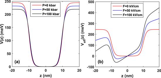
Figure 1. Scheme of the Woods–Saxon QW for (a) hydrostatic pressure P and (b) applied electric field F. |

Figure 2. Effect of the hydrostatic pressure P and applied electric field F on first four energy levels E0, E1, E2, E3 and the corresponding energy difference E10, E20, E30. |
The effect of the hydrostatic pressure P(a) and applied electric field F(b) on the THG ${\chi }_{3\omega }^{(3)}$ is shown in figure 3, as a function of incoming photon energies. As can be seen in figure 3(a), we see three resonant peaks in the THG susceptibilities in any curve. The first resonant peak is obtained when ℏω = E10, the second resonant peak is obtained when ℏω = E20/2, and the third resonant peak is located when ℏω = E30/3. The second resonant peak is more prominent than the other two resonant peaks in two cases. Moreover, it is clear that the THG ${\chi }_{3\omega }^{(3)}$ is strongly dependent on P. When only CEM is considered, one can see that all resonant peaks height of THG ${\chi }_{3\omega }^{(3)}$ increases as P increases, and the resonant peak position moves to lower energies (red-shift). This is explained by the reduction in quantum confinement. As concluded from the results depicted in figure 2. For the PDEM case, it is obvious from the figure that the increase of P will shift the resonant peak positions to a lower frequency due to the increase in the energy level interval. Moreover, the resonant peaks height of THG ${\chi }_{3\omega }^{(3)}$ also increases steadily with an increase in P. Figure 3(b) shows that the resonant peak heights of THG ${\chi }_{3\omega }^{(3)}$ appear discontinuous change considering CEM with the increase of F. When F = 50 kV cm−1, the peak values of THG ${\chi }_{3\omega }^{(3)}$ reaches the maximum value. It can also be noticed that the peak positions of the first and second resonant peaks are blue-shifted with the increase in F. However, the third resonant peak position displays non-uniform behavior, which is correct except for the case shown in figure 2(b). The overall behavior thus suggests that the resonant peaks of THG ${\chi }_{3\omega }^{(3)}$ sensitively depend on the mode of application of P and F for both CEM and PDEM cases, respectively. Thus, the influence of the PDEM must be considered in Woods–Saxon QW.

Figure 3. Effect of the hydrostatic pressure P (a) and applied electric field F (b) on the THG ${\chi }_{3\omega }^{(3)}$ with F = 0 kV cm−1 (a) and P = 0 kbar (b), respectively. |
The effect of the hydrostatic pressure P and applied electric field F on the linear α(1)(ω), the third-order nonlinear α(3)(ω) and the total OACs α(ω) is shown in figure 4, as a function of incoming photon energies. It is shown in figure 4(a), that the total OACs α(ω) showed a negative optical absorption for considering CEM. This is because the signs of the linear and nonlinear absorption term are opposite, the linear term will cause to increase α(ω), and the total change reduces by the nonlinear term. It is obvious that the peaks height of α(ω) decreases as P enhances. Meanwhile, the resonant peak positions of α(ω) shift towards lower energy regions (red-shift) as P increases. This is a consequence of the energy difference E10, which corresponds to the peak positions of α(1)(ω), α(3)(ω) and α(ω). One can observe from figure 4(b) that the peak's height of α(ω) is decreased when the P is increased for considering PDEM. This is due to the fact that the change of the peak values of α(1)(ω) is hardly noticeable, while the peak values of α(3)(ω) decrease with increasing P and there is a blue-shift, which can be attributed to the energy level spacing increases when P increases. By comparison of figures 4(a) and (b), it is important to note that PDEM plays an important role in the amplitude and position of the resonant peaks. Especially, when PDEM is taken into account, the position of the resonant peaks shifts in the opposite direction. From figure 4(c), one may notice that the resonant peaks show two peaks. This is due to the collapse of the total OACs α(ω) peak center caused by the nonlinear term. Meanwhile, it clearly seems that the peak height of α(ω) increases as F increases, additionally, it shifts to higher energies. This is explained by the increase of the subband energy difference with the increasing F. Figure 4(d) shows that the height and position of the resonant peaks with PDEM are comparable to the results with CEM. It is clear that the peak height of α(ω) increases as F increases. Additionally, the increment of F will lead to the change of the resonant peaks, in general as blue-shift, as concluded from the results depicted in figure 2(b).
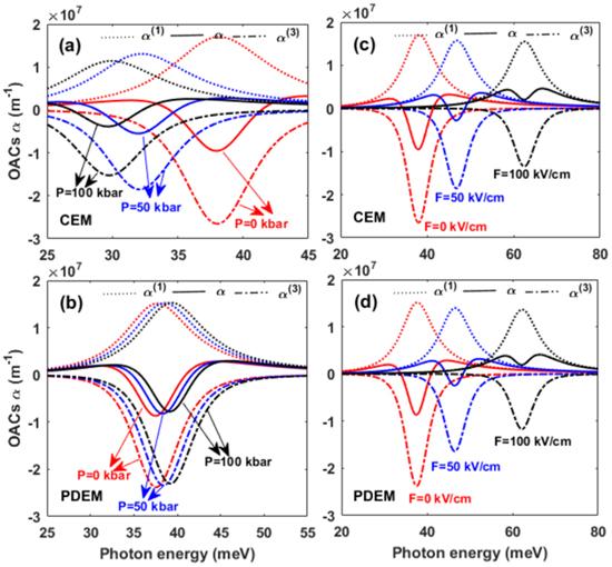
Figure 4. Effect of the hydrostatic pressure P and applied electric field F on the linear α(1)(ω), the third-order nonlinear α(3)(ω) and the total OACs α(ω), with F = 0 kV cm−1 (a, b) and P = 0 kbar (c, d), respectively. |
In order to obtain more complete information, It is necessary to study the nonlinear response to the incident light intensity. In figure 5, we have the total OACs α(ω) dependence on the photon energy both for the CEM (Solid line) and PDEM (Dash line) cases, respectively. One may notice that the peak height of α(ω) decreases for both the CEM and PDEM cases as the incident optical intensity increases. When incident optical intensity exceeds a critical value, the resonant peak of the α(ω) shows a transition from positive absorption to negative absorption. Furthermore, it is important to note that the PDEM effect on the peak values of α(ω) has a process from large to small and then from small to large with increasing incident optical intensity. However, no matter whether PDEM is considered or not, the critical value will not change.

Figure 5. The total OACs α(ω) versus incoming photon energies with CEM and PDEM, respectively. |
The effect of the hydrostatic pressure P and applied electric field F on the total RICs Δ/nr is shown in figure 6, as a function of incoming photon energies. As seen in figure 6(a), the peak values of total RICs Δ/nr decrease as P increases. Moreover, the corresponding peak positions of total RICs Δ/nr suffer a red-shift. The reason behind the said behavior is that the energy difference E10 decreases as P increases, similar to the features that have been discussed previously in figure 2(a). We also consider the PDEM in figure 6(b), the resonance peaks of total RICs Δ/nr tend to blue shifts as P increases, which shows a completely different change in comparison with the CEM case. This can be mutually confirmed with the results obtained in figure 2(b). Meanwhile, the peak values of total RICs Δ/nr decrease significantly for considering PDEM. Figure 6(c) shows that the resonant peaks of total RICs Δ/nr showed an increase in their heights or intensities, also the resonant peak positions of total RICs Δ/nr shift toward the higher energy regions due to the increasing energy difference E10. This is clearly seen in figure 2(d). Similar results can be discussed in figure 6(d), but only very slight differences from figure 6(c).

Figure 6. Effect of the hydrostatic pressure P and applied electric field F on the total RICs Δn/nr, with F = 0 kV cm−1 (a), (b) and P = 0 kbar (c), (d), respectively. |
4. Conclusions
In this study, numerical work has been performed to investigate the hydrostatic pressure and applied electric field on the THG susceptibility $| {\chi }_{3\omega }^{(3)}| $, linear and nonlinear OACs and RICs in an AlxGa1−xAs/GaAs Woods–Saxon QW with considering CEM and PDEM cases, respectively. To obtain the electric structures, the calculations were carried out by the finite difference method. The obtained meaningful results can be included as follows: (i) the peak height of the THG is an increase function of P for the CEM and PDEM case. Meanwhile, the resonant peaks of the THG susceptibility undergo a blue-shift with an increasing of P for the PDEM case, which is contrary to the conclusion only considering CEM. (ii) The peak values of the THG susceptibility increase significantly with increasing F, which experiences an obvious blue-shift for both cases CEM and PDEM due to an increment in the energy difference. (iii) The resonant peak positions of the total OACs showed red-shift and blue-shift as P increases for CEM and PDEM cases. (iv) When PDEM is considered, the applied electric field F has a more significant effect on the position of the resonant peaks of the total OACs. In addition, the effect of the electric field on total RICs is not obvious between the PDEM case and CEM case, but the static pressure conditions are the opposite. The sensitivity of the nonlinear THG, OACs, and RICs to hydrostatic pressure, applied electric field and PDEM are very useful for various applications of optoelectronic devices.