Welcome to visit Communications in Theoretical Physics,
Mathematical Physics

The Caputo–Fabrizio time-fractional Sharma–Tasso–Olver–Burgers equation and its valid approximations

  • Kamyar Hosseini 1, 2, ,
  • Mousa Ilie 1 ,
  • Mohammad Mirzazadeh , 3, ,
  • Dumitru Baleanu 4, 5 ,
  • Choonkil Park , 6, ,
  • Soheil Salahshour 7
Expand
  • 1Department of Mathematics, Rasht Branch, Islamic Azad University, Rasht, Iran
  • 2Department of Mathematics, Near East University TRNC, Mersin 10, Turkey
  • 3Department of Engineering Sciences, Faculty of Technology and Engineering, East of Guilan, University of Guilan, P.C. 44891-63157 Rudsar-Vajargah, Iran
  • 4Department of Mathematics, Faculty of Arts and Sciences, Cankaya University, Ankara, 06530, Turkey
  • 5 Institute of Space Sciences, Magurele-Bucharest, R 76900, Romania
  • 6Research Institute for Natural Sciences, Hanyang University, Seoul 04763, Republic of Korea
  • 7Faculty of Engineering and Natural Sciences, Bahcesehir University, Istanbul, Turkey

Authors to whom any correspondence should be addressed.

Received date: 2021-11-21

  Revised date: 2022-02-28

  Accepted date: 2022-04-01

  Online published: 2022-07-01

Copyright

© 2022 Institute of Theoretical Physics CAS, Chinese Physical Society and IOP Publishing

Abstract

Studying the dynamics of solitons in nonlinear time-fractional partial differential equations has received substantial attention, in the last decades. The main aim of the current investigation is to consider the time-fractional Sharma–Tasso–Olver–Burgers (STOB) equation in the Caputo–Fabrizio (CF) context and obtain its valid approximations through adopting a mixed approach composed of the homotopy analysis method (HAM) and the Laplace transform. The existence and uniqueness of the solution of the time-fractional STOB equation in the CF context are investigated by demonstrating the Lipschitz condition for $\varphi \left(x,t;u\right)$ as the kernel and giving some theorems. To illustrate the CF operator effect on the dynamics of the obtained solitons, several two- and three-dimensional plots are formally considered. It is shown that the mixed approach is capable of producing valid approximations to the time-fractional STOB equation in the CF context.

Cite this article

Kamyar Hosseini , Mousa Ilie , Mohammad Mirzazadeh , Dumitru Baleanu , Choonkil Park , Soheil Salahshour . The Caputo–Fabrizio time-fractional Sharma–Tasso–Olver–Burgers equation and its valid approximations[J]. Communications in Theoretical Physics, 2022 , 74(7) : 075003 . DOI: 10.1088/1572-9494/ac633e

1. Introduction

As we know, fractional calculus (FC) is a generalized version of classical calculus that relates to the derivative and integral of arbitrary order. FC is as old as classical calculus and has received much attention in the last few decades. Many studies with the theoretical discussion have been done within the framework of FC. So far, different fractional derivatives with singular and non-singular kernels have been proposed, some of these fractional derivatives are Riemann–Liouville derivative [1], Caputo derivative [2], Atangana–Baleanu derivative [3], and Caputo–Fabrizio (CF) derivative [4]. Veeresha and Prakasha [5] studied the time-fractional Zakharov–Kuznetsov equations in the Caputo sense and derived its approximate solutions with the help of the $q$-homotopy analysis transform method (HAMT). Yavuz et al [6] considered the time-fractional Schrödinger–KdV equation in the Atangana–Baleanu context and found its approximate solution through the modified Laplace decomposition method. Aydogan et al [7] explored the Rabies mathematical model in the CF sense and derived its approximate solutions through the Adomian decomposition method. For more studies, see [820].
The Sharma–Tasso–Olver–Burgers equation is a new nonlinear model that has been introduced by Yan and Lou in [21] and is expressed as
$\begin{eqnarray*}\begin{array}{l}{u}_{t}\left(x,t\right)+{c}_{1}\left(3{u}_{x}^{2}\left(x,t\right)+3{u}^{2}\left(x,t\right){u}_{x}\left(x,t\right)\right.\\ \left.\,+\,3u\left(x,t\right){u}_{xx}\left(x,t\right)+{u}_{xxx}\left(x,t\right)\right)\\ \,+\,{c}_{2}\left(2u\left(x,t\right){u}_{x}\left(x,t\right)+{u}_{xx}\left(x,t\right)\right)=0,\end{array}\end{eqnarray*}$
where ${c}_{1}$ and ${c}_{2}$ are free constants. It should be noted that the STOB equation is a combination of the STO and Burgers equations. Yan and Lou [21] obtained soliton molecules of the STOB equation using the velocity resonant mechanism. Miao et al [22] derived lump and interaction solutions of the STOB equation by adopting different test functions. Very recently, Hosseini et al [23] found kink solitons of the STOB equation through the exponential method. The main aim of the present study is to consider the time-fractional STOB equation in the CF context and obtain its valid approximations through adopting a mixed approach [2430] composed of the homotopy analysis method and the Laplace transform. The time-fractional STOB equation in the CF context can be written as follows
$\begin{eqnarray}\begin{array}{l}{}_{0}{}^{CF}D_{t}^{\alpha }u\left(x,t\right)+{c}_{1}\left(3{u}_{x}^{2}\left(x,t\right)+3{u}^{2}\left(x,t\right){u}_{x}\left(x,t\right)\right.\\ \left.\,+\,3u\left(x,t\right){u}_{xx}\left(x,t\right)+{u}_{xxx}\left(x,t\right)\right)\\ \,+\,{c}_{2}\left(2u\left(x,t\right){u}_{x}\left(x,t\right)+{u}_{xx}\left(x,t\right)\right)=0,0\lt \alpha \leqslant 1.\end{array}\end{eqnarray}$
The mixed approach namely the HAMT is a powerful analytical method that has been widely used to find valid approximations for nonlinear fractional equations. Aljhani et al [27] applied the HAMT to obtain a valid approximation of a fractional HIV model in the Caputo context. Baleanu et al [28] in their paper dealt with finding a valid approximation to a fractional model of COVID-19 in the CF sense using the HAMT. The authors of [29] derived a valid approximation to a fractional model of anthrax in the CF context through the HAMT. Very newly, Hosseini et al [30] utilized the HAMT to acquire valid approximations of a time-fractional nonlinear water wave equation in the Caputo sense.
With a close look at the research done in the above references, it can be concluded that the study of nonlinear fractional equations in the CF context is of particular importance in many branches of science. Therefore, here a series of required introductory definitions in the CF context that will be used in the next sections are provided.

Let $u\left(t\right)\in {H}^{1}\left(a,b\right),\,b\gt a$ and $\alpha \in \left(0,1\right).$ The fractional derivative of $u\left(t\right)$ of order $\alpha $ in the CF context is expressed as [4]

$\begin{eqnarray*}{}_{a}{}^{CF}D_{t}^{\alpha }u\left(t\right)=\displaystyle \frac{M\left(\alpha \right)}{1-\alpha }\displaystyle {\int }_{a}^{t}u^{\prime} \left(\varepsilon \right){{\rm{e}}}^{-\displaystyle \frac{\alpha }{1-\alpha }\left(t-\varepsilon \right)}{\rm{d}}\varepsilon ,\end{eqnarray*}$
with the properties $M\left(0\right)=M\left(1\right)=1.$

The fractional integral of $u\left(t\right)$ of order $\alpha $ in the CF sense is defined as [31]

$\begin{eqnarray*}\begin{array}{l}{}_{0}{}^{CF}I_{t}^{\alpha }u\left(t\right)=\displaystyle \frac{2\left(1-\alpha \right)}{\left(2-\alpha \right)M(\alpha )}u\left(t\right)+\displaystyle \frac{2\alpha }{\left(2-\alpha \right)M(\alpha )}\\ \,\,\,\,\,\times \,\displaystyle {\int }_{0}^{t}u\left(\varepsilon \right){\rm{d}}\varepsilon ,t\geqslant 0.\end{array}\end{eqnarray*}$

For a given expression like ${}_{0}{}^{CF}D_{t}^{\alpha }u\left(t\right),$ its Laplace transform can be written as [4]

$\begin{eqnarray*} {\mathcal L} \left[{}_{0}{}^{CF}D_{t}^{\alpha }u\left(t\right)\right]\left(s\right)=\displaystyle \frac{s {\mathcal L} \left[u\left(t\right)\right]\left(s\right)-u(0)}{s+\alpha \left(1-s\right)},\end{eqnarray*}$
and generally,
$\begin{eqnarray*}\begin{array}{l} {\mathcal L} \left[{{}_{0}{}^{CF}D}_{t}^{\left(\alpha +n\right)}u\left(t\right)\right]\left(s\right)\\ \,=\displaystyle \frac{{s}^{n+1} {\mathcal L} \left[u\left(t\right)\right]\left(s\right)-{s}^{n}u\left(0\right)-{s}^{n-1}u^{\prime} \left(0\right)-\cdots -{u}^{\left(n\right)}\left(0\right)}{s+\alpha \left(1-s\right)}.\end{array}\end{eqnarray*}$
The outline of this paper is as follows: In section 2, the existence and uniqueness of the solution of the time-fractional STOB equation in the CF context are investigated by demonstrating the Lipschitz condition for $\varphi (x,\,t;u)$ as the kernel and giving some theorems. In section 3, valid approximations of the time-fractional STOB equation in the CF context are derived through adopting the HAMT. In section 4, the effectiveness of the HATM in handling the time-fractional STOB equation in the CF context is shown. Additionally, the CF operator effect on the dynamics of the obtained solitons is investigated in detail. The outcomes of the present investigation are given in the last section.

2. The theoretical discussion on the existence and uniqueness of the solution

Supposing
$\begin{eqnarray*}\begin{array}{l}\varphi \left(x,t;u\right)=-\left({c}_{1}\left(3{u}_{x}^{2}\left(x,t\right)+3{u}^{2}\left(x,t\right){u}_{x}\left(x,t\right)\right.\right.\\ \left.\,+\,3u\left(x,t\right){u}_{xx}\left(x,t\right)+{u}_{xxx}\left(x,t\right)\right)\\ \left.\,+\,{c}_{2}\left(2u\left(x,t\right){u}_{x}\left(x,t\right)+{u}_{xx}\left(x,t\right)\right)\right),\end{array}\end{eqnarray*}$
recommends that equation (1) can be rewritten as
$\begin{eqnarray*}{}_{0}{}^{CF}D_{t}^{\alpha }u\left(x,t\right)=\varphi \left(x,t;u\right).\end{eqnarray*}$

Assume that $u(x,\,t)$ and $v(x,\,t)$ are the bounded functions, namely $\parallel u\parallel \leqslant \mu $ and $\parallel v\parallel \leqslant \upsilon .$ Then, $\varphi \left(x,t;u\right)$ is a kernel satisfying the Lipschitz condition.

Proof.
$\begin{eqnarray*}\parallel \varphi \left(x,t;u\right)-\varphi \left(x,t;v\right)\parallel \end{eqnarray*}$
$\begin{eqnarray*}\begin{array}{l}=\,\parallel 3{c}_{1}\left({u}_{x}^{2}-{v}_{x}^{2}\right)+3{c}_{1}\left({u}^{2}{u}_{x}-{v}^{2}{v}_{x}\right)\\ +3{c}_{1}\left(u{u}_{xx}-v{v}_{xx}\right)+{c}_{1}\left({u}_{xxx}-{v}_{xxx}\right)\\ +{c}_{2}\left(2u{u}_{x}-2v{v}_{x}\right)+{c}_{2}\left({u}_{xx}-{v}_{xx}\right)\parallel \end{array}\end{eqnarray*}$
$\begin{eqnarray*}\begin{array}{l}=\parallel 3{c}_{1}\displaystyle \frac{\partial }{\partial x}\left(u-v\right)\displaystyle \frac{\partial }{\partial x}\left(u+v\right)+{c}_{1}\displaystyle \frac{\partial }{\partial x}\left({u}^{3}-{v}^{3}\right)\\ +3{c}_{1}\left(u\displaystyle \frac{{\partial }^{2}u}{\partial {x}^{2}}-u\displaystyle \frac{{\partial }^{2}v}{\partial {x}^{2}}+u\displaystyle \frac{{\partial }^{2}v}{\partial {x}^{2}}-v\displaystyle \frac{{\partial }^{2}v}{\partial {x}^{2}}\right)\\ +{c}_{1}\displaystyle \frac{{\partial }^{3}}{\partial {x}^{3}}\left(u-v\right)+{c}_{2}\displaystyle \frac{\partial }{\partial x}\left({u}^{2}-{v}^{2}\right)+{c}_{2}\displaystyle \frac{{\partial }^{2}}{\partial {x}^{2}}\left(u-v\right)\parallel \end{array}\end{eqnarray*}$
$\begin{eqnarray*}\begin{array}{l}=\,\parallel 3{c}_{1}\displaystyle \frac{\partial }{\partial x}\left(u-v\right)\displaystyle \frac{\partial }{\partial x}\left(u+v\right)+{c}_{1}\left({u}^{2}+uv+{v}^{2}\right)\\ \times \,\displaystyle \frac{\partial }{\partial x}\left(u-v\right)+{c}_{1}\left(u-v\right)\displaystyle \frac{\partial }{\partial x}\left({u}^{2}+uv+{v}^{2}\right)\\ +3{c}_{1}u\displaystyle \frac{{\partial }^{2}}{\partial {x}^{2}}\left(u-v\right)+3{c}_{1}\left(u-v\right)\displaystyle \frac{{\partial }^{2}v}{\partial {x}^{2}}\\ +{c}_{1}\displaystyle \frac{{\partial }^{3}}{\partial {x}^{3}}\left(u-v\right)+{c}_{2}\left(u+v\right)\displaystyle \frac{\partial }{\partial x}\left(u-v\right)\\ +{c}_{2}\left(u-v\right)\displaystyle \frac{\partial }{\partial x}\left(u+v\right)+{c}_{2}\displaystyle \frac{{\partial }^{2}}{\partial {x}^{2}}\left(u-v\right)\parallel \\ \leqslant \,3| {c}_{1}| \parallel \displaystyle \frac{\partial }{\partial x}\left(u-v\right)\parallel \parallel \displaystyle \frac{\partial }{\partial x}\left(u+v\right)\parallel +\left|{c}_{1}\right|\parallel {u}^{2}+uv+{v}^{2}\parallel \parallel \displaystyle \frac{\partial }{\partial x}\left(u-v\right)\parallel \\ +\left|{c}_{1}\right|\parallel u-v\parallel \parallel \displaystyle \frac{\partial }{\partial x}\left({u}^{2}+uv+{v}^{2}\right)\parallel +3\left|{c}_{1}\right|\parallel u\parallel \parallel \displaystyle \frac{{\partial }^{2}}{\partial {x}^{2}}\left(u-v\right)\parallel \\ +3\left|{c}_{1}\right|\parallel u-v\parallel \parallel \displaystyle \frac{{\partial }^{2}v}{\partial {x}^{2}}\parallel +\left|{c}_{1}\right|\parallel \displaystyle \frac{{\partial }^{3}}{\partial {x}^{3}}\left(u-v\right)\parallel +\left|{c}_{2}\right|\parallel u\\ +v\parallel \parallel \displaystyle \frac{\partial }{\partial x}\left(u-v\right)\parallel +\left|{c}_{2}\right|\parallel u-v\parallel \parallel \displaystyle \frac{\partial }{\partial x}\left(u+v\right)\parallel +\left|{c}_{2}\right|\parallel \displaystyle \frac{{\partial }^{2}}{\partial {x}^{2}}\left(u-v\right)\parallel \end{array}\end{eqnarray*}$
$\begin{eqnarray*}\begin{array}{l}\leqslant 3\left|{c}_{1}\right|A\parallel u-v\parallel \parallel u+v\parallel +\left|{c}_{1}\right|B\parallel {u}^{2}+uv+{v}^{2}\parallel \parallel u-v\parallel \\ +\left|{c}_{1}\right|C\parallel u-v\parallel \parallel {u}^{2}+uv+{v}^{2}\parallel +3\left|{c}_{1}\right|D\parallel u\parallel \parallel u-v\parallel +3\left|{c}_{1}\right|E\parallel u-v\parallel \parallel v\parallel \\ +\left|{c}_{1}\right|F\parallel u-v\parallel +\left|{c}_{2}\right|G\parallel u+v\parallel \parallel u-v\parallel +\left|{c}_{2}\right|H\parallel u-v\parallel \parallel u+v\parallel \\ +\left|{c}_{2}\right|K\parallel u-v\parallel \leqslant 3\left|{c}_{1}\right|A\left(\mu +\upsilon \right)\\ \parallel \parallel u-v\parallel +\left|{c}_{1}\right|B\left({\mu }^{2}+\mu \upsilon +{\upsilon }^{2}\right)\parallel u-v\parallel +\left|{c}_{1}\right|\\ \times C\left({\mu }^{2}+\mu \upsilon +{\upsilon }^{2}\right)\parallel u-v\parallel +3\left|{c}_{1}\right|D\mu \parallel u-v\parallel \\ +3\left|{c}_{1}\right|E\upsilon \parallel u-v\parallel +\left|{c}_{1}\right|F\parallel u-v\parallel +\left|{c}_{2}\right|G\left(\mu +\upsilon \right)\\ \times \parallel u-v\parallel +\left|{c}_{2}\right|H\left(\mu +\upsilon \right)\parallel u-v\parallel +\left|{c}_{2}\right|K\parallel u-v\parallel \end{array}\end{eqnarray*}$
$\begin{eqnarray*}\begin{array}{l}=\left(\left(3\left|{c}_{1}\right|A+\left|{c}_{2}\right|\left(G+H\right)\right)\left(\mu +\upsilon \right)+\left|{c}_{1}\right|\left(B+C\right)\right.\\ \times \left({\mu }^{2}+\mu \upsilon +{\upsilon }^{2}\right)+3\left|{c}_{1}\right|(D\mu +E\upsilon )+\left|{c}_{1}| F\right|\\ \left.+\left|{c}_{2}\right|K\right)\parallel u-v\parallel .\end{array}\end{eqnarray*}$
Now, assuming
$\begin{eqnarray*}\begin{array}{l}\lambda =\left.3\left|{c}_{1}\right|A+\left|{c}_{2}\right|\left(G+H\right)\right)\left(\mu +\upsilon \right)+\left|{c}_{1}\right|\left(B+C\right)\\ \times \left({\mu }^{2}+\mu \upsilon +{\upsilon }^{2}\right)+3\left|{c}_{1}\right|\left(D\mu +E\upsilon \right)+\left|{c}_{1}\right|F+\left|{c}_{2}\right|K,\end{array}\end{eqnarray*}$
yields
$\begin{eqnarray*}\parallel \varphi \left(x,t;u\right)-\varphi (x,t;v)\parallel \leqslant \lambda \parallel u-v\parallel ,\end{eqnarray*}$
which is the desired result.

If at $t={t}_{0},$ we have

$\begin{eqnarray*}0\leqslant \displaystyle \frac{2\left(1-\alpha \right)}{\left(2-\alpha \right)M(\alpha )}\lambda +\displaystyle \frac{2\alpha }{\left(2-\alpha \right)M(\alpha )}\lambda {t}_{0}\lt 1,\end{eqnarray*}$
then, the solution of the time-fractional STOB equation in the CF context exists.

See [25] and its references.

If at $t={t}_{0},$ we have.

$\begin{eqnarray*}0\leqslant \displaystyle \frac{2\left(1-\alpha \right)}{\left(2-\alpha \right)M(\alpha )}\lambda +\displaystyle \frac{2\alpha }{\left(2-\alpha \right)M(\alpha )}\lambda {t}_{0}\lt 1,\end{eqnarray*}$
then, the solution of the time-fractional STOB equation in the CF context is unique.

See [25] and its references.

3. Analytical solutions to the time-fractional STOB equation in the CF context

The authors' purpose in the current section is to establish analytical solutions of the time-fractional STOB equation in the CF context. In this respect, first solitons of the STOB equation are derived with the help of ansatz method. The HATM is then employed to extract approximate solutions of the time-fractional STOB equation in the CF context. The computations are handled by Maple software.

3.1. The STOB equation and its solitons

To start, we consider a test function as [3234]
$\begin{eqnarray}u\left(x,t\right)={A}_{0}+{A}_{1}\,\tanh \left(kx+wt\right),\end{eqnarray}$
where ${A}_{0}$ and ${A}_{1}$ are unknowns. Inserting equation (2) into the SOTB equation results in
$\begin{eqnarray*}\begin{array}{l}\left(-4{k}^{3}{c}_{1}+6{k}^{2}{A}_{1}{c}_{1}-3k{A}_{0}^{2}{c}_{1}-3k{A}_{1}^{2}{c}_{1}\right.\\ \left.-2k{A}_{0}{c}_{2}-w\right)\cos \,\,{{\rm{h}}}^{2}\left(kx+wt\right)+\left(6{k}^{2}{A}_{0}{c}_{1}\right.\\ \left.-6k{A}_{0}{A}_{1}{c}_{1}+2{k}^{2}{c}_{2}-2k{A}_{1}{c}_{2}\right)\cos \,\,{\rm{h}}\left(kx+wt\right)\\ \sin \,\,{\rm{h}}\left(kx+wt\right)+6{k}^{3}{c}_{1}-9{k}^{2}{A}_{1}{c}_{1}+3k{A}_{1}^{2}{c}_{1}=0.\end{array}\end{eqnarray*}$
From the above expression, the following system of nonlinear algebraic equations is obtained
$\begin{eqnarray*}-4{k}^{3}{c}_{1}+6{k}^{2}{A}_{1}{c}_{1}-3k{A}_{0}^{2}{c}_{1}-3k{A}_{1}^{2}{c}_{1}-2k{A}_{0}{c}_{2}-w=0,\end{eqnarray*}$
$\begin{eqnarray*}6{k}^{2}{A}_{0}{c}_{1}-6k{A}_{0}{A}_{1}{c}_{1}+2{k}^{2}{c}_{2}-2k{A}_{1}{c}_{2}=0,\end{eqnarray*}$
$\begin{eqnarray*}6{k}^{3}{c}_{1}-9{k}^{2}{A}_{1}{c}_{1}+3k{A}_{1}^{2}{c}_{1}=0.\end{eqnarray*}$
The above system is solved to get the following cases:
Case 1
$\begin{eqnarray*}{A}_{1}=k,\,w=-{k}^{3}{c}_{1}-3k{A}_{0}^{2}{c}_{1}-2k{A}_{0}{c}_{2}.\end{eqnarray*}$
Therefore, the following soliton to the SOTB equation is derived
$\begin{eqnarray*}\begin{array}{l}{u}_{1}\left(x,t\right)\\ =\,{A}_{0}+k\,\tanh \left(kx-\left({k}^{3}{c}_{1}+3k{A}_{0}^{2}{c}_{1}+2k{A}_{0}{c}_{2}\right)t\right),\end{array}\end{eqnarray*}$
where for ${A}_{0}=1,$ ${c}_{1}=1,$ ${c}_{2}=1,$ and $k=1$ is changed into
$\begin{eqnarray}{u}_{1}\left(x,t\right)=1+\,\tanh \left(x-6t\right),\end{eqnarray}$
with a series representation as
$\begin{eqnarray*}{u}_{1}\left(x,t\right)=1-\displaystyle \frac{{{\rm{e}}}^{-2x}-1}{{{\rm{e}}}^{-2x}+1}-24\displaystyle \frac{{{\rm{e}}}^{-2x}}{{\left({{\rm{e}}}^{-2x}+1\right)}^{2}}t+\cdots .\end{eqnarray*}$
Case 2
$\begin{eqnarray*}{A}_{0}=-\displaystyle \frac{{c}_{2}}{3{c}_{1}},{A}_{1}=2k,w=-\displaystyle \frac{k\left(12{k}^{2}{c}_{1}^{2}-{c}_{2}^{2}\right)}{3{c}_{1}}.\end{eqnarray*}$
Thus, the following soliton to the SOTB equation is obtained
$\begin{eqnarray}\begin{array}{l}{u}_{2}\left(x,t\right)=-\displaystyle \frac{{c}_{2}}{3{c}_{1}}+2k\,\tanh \,\left(kx-\displaystyle \frac{k\left(12{k}^{2}{c}_{1}^{2}-{c}_{2}^{2}\right)}{3{c}_{1}}t\right),\end{array}\end{eqnarray}$
where for ${c}_{1}=1,$ ${c}_{2}=1,$ and $k=1$ can be written
$\begin{eqnarray*}{u}_{2}\left(x,t\right)=-\,\displaystyle \frac{1}{3}+2\,\tanh \left(x-\displaystyle \frac{11}{3}t\right),\end{eqnarray*}$
with the following series representation
$\begin{eqnarray*}{u}_{2}\left(x,t\right)=-\displaystyle \frac{1}{3}-2\displaystyle \frac{{{\rm{e}}}^{-2x}-1}{{{\rm{e}}}^{-2x}+1}-\displaystyle \frac{88{{\rm{e}}}^{-2x}}{3{\left({{\rm{e}}}^{-2x}+1\right)}^{2}}t+\cdots .\end{eqnarray*}$

3.2. The time-fractional STOB equation in the CF context and its approximate solutions

By considering ${c}_{1}=1$ and ${c}_{2}=1$ (selected by the authors) in equation (1) and adopting the Laplace transform, we find
$\begin{eqnarray}\begin{array}{l} {\mathcal L} \left[u\left(x,t\right)\right]-\displaystyle \frac{u\left(x,0\right)}{s}+\displaystyle \frac{s+\alpha \left(1-s\right)}{s} {\mathcal L} \left[3{u}_{x}^{2}\left(x,t\right)\right.\\ +\,3{u}^{2}\left(x,t\right){u}_{x}\left(x,t\right)+3u\left(x,t\right){u}_{xx}\left(x,t\right)+{u}_{xxx}\left(x,t\right)\\ \left.+\,2u\left(x,t\right){u}_{x}\left(x,t\right)+{u}_{xx}\left(x,t\right)\right]\,=0.\end{array}\end{eqnarray}$
Equation (5) recommends considering the following nonlinear operator
$\begin{eqnarray*}\begin{array}{l}{\rm{\Phi }}\left[\psi \left(x,t;p\right)\right]= {\mathcal L} \left[\psi \left(x,t;p\right)\right]-\frac{\psi \left(x,0;p\right)}{s}\\ +\frac{s+\alpha \left(1-s\right)}{s} {\mathcal L} \left[3{\psi }_{x}^{2}\left(x,t;p\right)+3{\psi }^{2}\left(x,t;p\right)\right.{\psi }_{x} \left(x,t;p\right)\\ +3\psi \left(x,t;p\right){\psi }_{xx}\left(x,t;p\right)+{\psi }_{xxx}\left(x,t;p\right)\\ \left.+2\psi \left(x,t;p\right){\psi }_{x}\left(x,t;p\right)+{\psi }_{xx}\left(x,t;p\right)\right].\end{array}\end{eqnarray*}$
Based on the HAM [35], the following mth order deformation equation is formally constructed
$\begin{eqnarray*} {\mathcal L} \left[{u}_{m}\left(x,t\right)-{\chi }_{m}{u}_{m-1}(x,t)\right]=h{{\mathscr{Q}}}_{m}\left({\vec{u}}_{m-1}\right),\end{eqnarray*}$
where
$\begin{eqnarray*}{{\mathscr{Q}}}_{m}\left({\vec{u}}_{m-1}\right)=\displaystyle \frac{1}{\left(m-1\right)!}{\left.\displaystyle \frac{{\partial }^{m-1}{\rm{\Phi }}\left[\psi \left(x,t;p\right)\right]}{\partial {p}^{m-1}}\right|}_{p=0},\end{eqnarray*}$
and
$\begin{eqnarray*}{\chi }_{m}=\left\{\begin{array}{c}0\, & m\leqslant 1,\\ 1\, & m\gt 1.\end{array}\right.\end{eqnarray*}$
In the first step, suppose that the initial condition of the time-fractional STOB equation in the CF context when ${c}_{1}=1$ and ${c}_{2}=1$ is as follows
$\begin{eqnarray*}u\left(x,0\right)=1-\displaystyle \frac{{{\rm{e}}}^{-2x}-1}{{{\rm{e}}}^{-2x}+1}.\end{eqnarray*}$
Considering the above initial condition and solving the resultant equations successively, yields
$\begin{eqnarray*}{u}_{0}\left(x,t\right)=1-\displaystyle \frac{{{\rm{e}}}^{-2x}-1}{{{\rm{e}}}^{-2x}+1},\end{eqnarray*}$
$\begin{eqnarray*}{u}_{1}\left(x,t\right)=\displaystyle \frac{24h\left(\alpha t-\alpha +1\right){{\rm{e}}}^{-2x}}{{\left({{\rm{e}}}^{-2x}+1\right)}^{2}},\cdots .\end{eqnarray*}$
Consequently, the following series solution to the time-fractional STOB equation in the CF context is gained
$\begin{eqnarray*}{u}_{1}\left(x,t\right)=1-\displaystyle \frac{{{\rm{e}}}^{-2x}-1}{{{\rm{e}}}^{-2x}+1}+\displaystyle \frac{24h\left(\alpha t-\alpha +1\right){{\rm{e}}}^{-2x}}{{\left({{\rm{e}}}^{-2x}+1\right)}^{2}}+\cdots .\end{eqnarray*}$
In the special case when $\alpha =1$ and $h=-1,$ one can obtain
$\begin{eqnarray*}{u}_{1}\left(x,t\right)=1-\displaystyle \frac{{{\rm{e}}}^{-2x}-1}{{{\rm{e}}}^{-2x}+1}-24\displaystyle \frac{{{\rm{e}}}^{-2x}}{{\left({{\rm{e}}}^{-2x}+1\right)}^{2}}t+\cdots ,\end{eqnarray*}$
with a closed-form representation as
$\begin{eqnarray*}{u}_{1}\left(x,t\right)=1+\,\tanh \left(x-6t\right).\end{eqnarray*}$
Now, assume that the initial condition of the time-fractional STOB equation in the CF context when ${c}_{1}=1$ and ${c}_{2}=1$ is as follows
$\begin{eqnarray*}u\left(x,0\right)=-\displaystyle \frac{1}{3}-2\displaystyle \frac{{{\rm{e}}}^{-2x}-1}{{{\rm{e}}}^{-2x}+1}.\end{eqnarray*}$
By considering the above initial condition and solving the resultant equations successively, one can find
$\begin{eqnarray*}{u}_{0}\left(x,t\right)=-\displaystyle \frac{1}{3}-2\displaystyle \frac{{{\rm{e}}}^{-2x}-1}{{{\rm{e}}}^{-2x}+1},\end{eqnarray*}$
$\begin{eqnarray*}{u}_{1}\left(x,t\right)=\displaystyle \frac{88h\left(\alpha t-\alpha +1\right){{\rm{e}}}^{-2x}}{3{\left({{\rm{e}}}^{-2x}+1\right)}^{2}},\cdots .\end{eqnarray*}$
Consequently, a series solution to the time-fractional STOB equation in the CF context is acquired as
$\begin{eqnarray*}\begin{array}{l}{u}_{2}\left(x,t\right)=-\displaystyle \frac{1}{3}-2\displaystyle \frac{{{\rm{e}}}^{-2x}-1}{{{\rm{e}}}^{-2x}+1}+\displaystyle \frac{88h\left(\alpha t-\alpha +1\right){{\rm{e}}}^{-2x}}{3{\left({{\rm{e}}}^{-2x}+1\right)}^{2}}\\ +\cdots .\end{array}\end{eqnarray*}$
In the special case when $\alpha =1$ and $h=-1,$ one can derive
$\begin{eqnarray*}{u}_{2}\left(x,t\right)=-\displaystyle \frac{1}{3}-2\displaystyle \frac{{{\rm{e}}}^{-2x}-1}{{{\rm{e}}}^{-2x}+1}-\displaystyle \frac{88{{\rm{e}}}^{-2x}}{3{\left({{\rm{e}}}^{-2x}+1\right)}^{2}}t+\cdots ,\end{eqnarray*}$
with the following closed-form representation
$\begin{eqnarray*}{u}_{2}\left(x,t\right)=-\displaystyle \frac{1}{3}+2\,\tanh \left(x-\displaystyle \frac{11}{3}t\right).\end{eqnarray*}$

(Convergence analysis) [36]: The series $u\left(x,t\right)\,={u}_{0}\left(x,t\right)+\displaystyle {\sum }_{k=1}^{+\infty }{u}_{k}\left(x,t\right)$ is convergence if $\exists \,0\lt r\lt 1$ such that $\parallel {u}_{k+1}\parallel \leqslant r\parallel {u}_{k}\parallel $ for all $k\geqslant {k}_{0}$ and for some ${k}_{0}\in {\mathbb{N}}.$

Moreover, the estimated error can be given as
$\begin{eqnarray*}\parallel u-\displaystyle \sum _{k=0}^{m}{u}_{k}\parallel \leqslant \displaystyle \frac{{r}^{m+1}}{1-r}\parallel {u}_{0}\parallel .\end{eqnarray*}$

4. Simulations and discussion

In this section, several two- and three-dimensional plots are considered to illustrate the CF operator effect on the dynamics of the obtained solitons. Figure 1 shows the two-dimensional plot of the 4th order approximation for $t=0.001,$ $h=-1,$ and $\alpha =1,$ $0.98,$ and $0.96$ (Selected by the authors). The CF operator effect on the dynamics of the kink soliton is formally observed from this figure. Additionally, by referring to figure 1 again, it can be observed that the results of the 4th order approximation and the exact solution (equation (3)) are in compromise. The three-dimensional plots of the 4th order approximation have been given in figure 2 for $h=-1$ and $\alpha =1,$ $0.98,$ and $0.96.$ Table 1 presents the absolute error of the 4th order approximation ($h=-1$) and the exact solution (equation (3)) when ${x}_{i}=0.5i,\,i=0,1,\mathrm{...},10$ and $t=0.001.$ The results confirm the potential of the HATM in handling the time-fractional STOB equation in the CF context. The two-dimensional plot of the 4th order approximation for $t=0.001,$ $h=-1,$ and $\alpha =1,$ $0.98,$ and $0.96$ has been illustrated in figure 3. From this figure, the CF operator effect on the dynamics of the kink soliton is clearly seen. Furthermore, by looking at figure 3 again, it can be seen that the results of the 4th order approximation and the exact solution (equation (4)) are in compromise. The three-dimensional plots corresponding to the 4th order approximation have been represented in figure 4 for $h=-1$ and $\alpha =1,$ $0.98,$ and $0.96.$ Table 2 demonstrates the absolute error of the 4th order approximation ($h=-1$) and the exact solution (equation (4)) when ${x}_{i}=0.5i,\,i=0,1,\mathrm{...},10$ and $t=0.001.$ Based on the results presented in table 2, the utility of the HATM in dealing with the time-fractional STOB equation in the CF context is confirmed.
Figure 1. The first exact solution ($t=0.001$) against the 4th order approximation for $t=0.001,$ h = −1, and $\alpha =1,$ $0.98,$ and $0.96.$
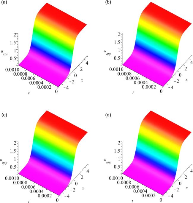
Figure 2. (a) The first exact solution against (b) the 4th order approximation for $\alpha =1$ and $h=-1$ (c) the 4th order approximation for $\alpha =0.98$ and $h=-1$ (d) the 4th order approximation for $\alpha =0.96$ and $h=-1$.
Table 1. The absolute error of the 8th order approximation and the first exact solution.
${x}$ The 8th order approximation when ${t}=0.001,$ ${h}=-1,$ and ${\alpha }=1$ The first exact solution when ${t}=0.001$ and ${\alpha }=1$ The absolute error
$0$ $0.994000072$ $0.994000072$ $0$
$0.5$ $1.457385408$ $1.457385408$ $0$
$1$ $1.759062773$ $1.759062773$ $0$
$1.5$ $1.904058107$ $1.904058106$ $1\times {10}^{-9}$
$2$ $1.963601214$ $1.963601214$ $0$
$2.5$ $1.986453796$ 1. $986453797$ $1\times {10}^{-9}$
$3$ $1.994995203$ $1.994995203$ $0$
$3.5$ $1.998155921$ $1.998155921$ $0$
$4$ $1.999321205$ $1.999321206$ $1\times {10}^{-9}$
$4.5$ $1.999750232$ $1.999750232$ $0$
$5$ $1.999908108$ $1.999908108$ $0$
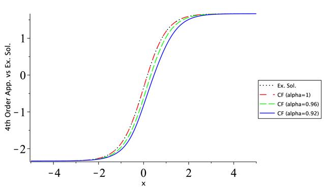
Figure 3. The second exact solution ($t=0.001$) against the 4th order approximation for $t=0.001,$ $h=-1,$ and $\alpha =1,$ $0.96,$ and $0.92.$
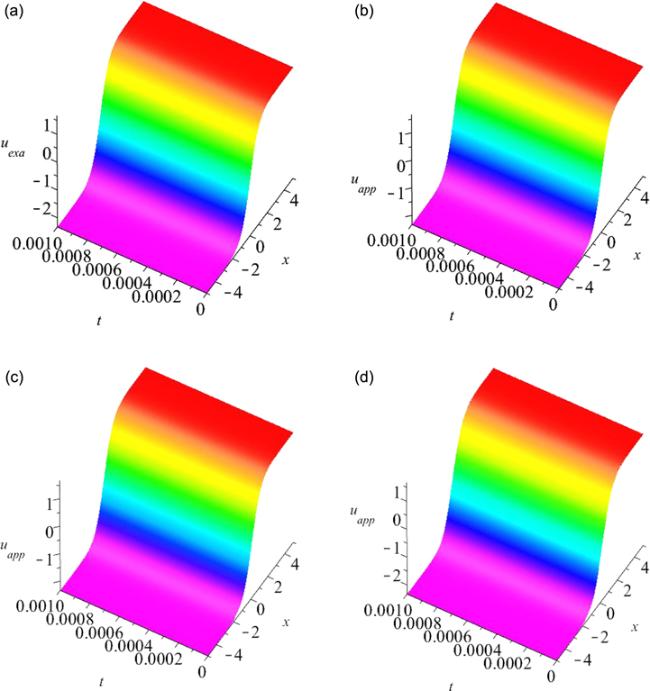
Figure 4. (a) The second exact solution against (b) the 4th order approximation for $\alpha =1$ and $h=-1$ (c) the 4th order approximation for $\alpha =0.96$ and $h=-1$ (d) the 4th order approximation for $\alpha =0.92$ and $h=-1$.
Table 2. The absolute error of the 8th order approximation and the second exact solution.
${x}$ The 8th order approximation when ${t}=0.001,$ ${h}=-1,$ and ${\alpha }=1$ The second exact solution when ${t}=0.001$ and ${\alpha }=1$ The absolute error
$0$ $-0.340666633$ $-0.340666633$ $0$
$0.5$ $0.5851239350$ $0.5851239349$ $1\times {10}^{-10}$
$1$ $1.186766556$ $1.186766556$ $0$
$1.5$ $1.475633586$ $1.475633585$ $1\times {10}^{-9}$
$2$ $1.594201885$ $1.594201886$ $1\times {10}^{-9}$
$2.5$ $1.639699546$ $1.639699546$ $0$
$3$ $1.656703559$ $1.656703559$ $0$
$3.5$ $1.662995664$ $1.662995664$ $0$
$4$ $1.665315396$ $1.665315397$ $1\times {10}^{-9}$
$4.5$ $1.666169455$ $1.666169456$ $1\times {10}^{-9}$
$5$ $1.666483738$ $1.666483739$ $1\times {10}^{-9}$

5. Conclusion

As it was stated, exploring the dynamics of solitons in nonlinear time-fractional partial differential equations has gained considerable interest, in the last decades. The key objective of the current study was to consider the time-fractional STOB equation in the CF context and acquire its valid approximations through utilizing a mixed approach composed of the HAM and the Laplace transform. The existence and uniqueness of the solution of the time-fractional STOB equation in the CF context were analyzed by proving the Lipschitz condition for $\varphi (x,\,t;u)$ as the kernel and providing some theorems. To demonstrate the CF operator effect on the dynamics of the obtained solitons, several two- and three-dimensional plots were portrayed. It was observed that the mixed approach is capable of generating valid approximations to the time-fractional STOB equation in the CF context.

Declaration of competing interest

The authors declare no conflict of interest.

Competing interests

The authors declare that they have no competing interests.

1
Podlubny I 1999 Fractional Differential Equations New York Academic

2
Caputo M 1967 Linear models of dissipation whose $Q$ is almost frequency independent: II Geophys. J. R. Astron. Soc. 13 529 539

DOI

3
Atangana A Baleanu D 2016 New fractional derivative with nonlocal and non-singular kernel, theory and application to heat transfer model Therm. Sci. 20 763 769

DOI

4
Caputo M Fabrizio M 2015 A new definition of fractional derivative without singular kernel Prog. Fract. Differ. Appl. 1 73 85

5
Veeresha P Prakasha D G 2019 Solution for fractional Zakharov–Kuznetsov equations by using two reliable techniques Chin. J. Phys. 60 313 330

DOI

6
Yavuz M Sulaiman T A Yusuf A Abdeljawad T 2021 The Schrödinger–KdV equation of fractional order with Mittag–Leffler nonsingular kernel Alexandria Eng. J. 60 2715 2724

DOI

7
Aydogan S M Baleanu D Mohammadi H Rezapour S 2020 On the mathematical model of Rabies by using the fractional Caputo–Fabrizio derivative Adv. Differ. Equ. 2020 382

DOI

8
Baleanu D Mohammadi H Rezapour S 2020 Analysis of the model of HIV-1 infection of CD4+ T-cell with a new approach of fractional derivative Adv. Differ. Equ. 2020 71

DOI

9
Baleanu D Jajarmi A Mohammadi H Rezapour S 2020 A new study on the mathematical modelling of human liver with Caputo–Fabrizio fractional derivative Chaos, Solitons Fractals 134 109705

10
Shah K Jarad F Abdeljawad T 2020 On a nonlinear fractional order model of dengue fever disease under Caputo–Fabrizio derivative Alexandria Eng. J. 59 2305 2313

DOI

11
Inc M Yusuf A Aliyu A I Baleanu D 2018 Investigation of the logarithmic-KdV equation involving Mittag–Leffler type kernel with Atangana–Baleanu derivative Physica A 506 520 531

DOI

12
Korpinar Z Inc M Bayram M 2020 Theory and application for the system of fractional burger equations with Mittag Leffler kernel Appl. Math. Comput. 367 124781

DOI

13
Gao W Veeresha P Prakasha D G Baskonus H M Yel G 2019 A powerful approach for fractional Drinfeld–Sokolov–Wilson equation with Mittag–Leffler law Alexandria Eng. J. 58 1301 1311

DOI

14
Yusuf A Inc M Aliyu A I Baleanu D 2018 Efficiency of the new fractional derivative with nonsingular Mittag–Leffler kernel to some nonlinear partial differential equations Chaos, Solitons Fractals 116 220 226

DOI

15
Bhatter S Mathur A Kumar D Nisar K S Singh J 2020 Fractional modified Kawahara equation with Mittag–Leffler law Chaos, Solitons Fractals 131 109508

16
Prakasha D G Veeresha P Baskonus H M 2019 Analysis of the dynamics of hepatitis E virus using the Atangana–Baleanu fractional derivative Eur. Phys. J. Plus 134 241

DOI

17
Yavuz M 2022 European option pricing models described by fractional operators with classical and generalized Mittag–Leffler kernels Numer. Methods Partial Differ. Equ. 38 434 456

DOI

18
Yavuz M Ozdemir N 2018 Numerical inverse Laplace homotopy technique for fractional heat equations Therm. Sci. 22 185 194

DOI

19
Boulaaras S Jan R Khan A Ahsan M 2022 Dynamical analysis of the transmission of dengue fever via Caputo–Fabrizio fractional derivative Chaos, Solitons Fractals: X 8 100072

DOI

20
El-Sayed A A E Boulaaras S Sweilam N H 2021 Numerical solution of the fractional‐order logistic equation via the first‐kind Dickson polynomials and spectral tau method Math. Methods Appl. Sci.

DOI

21
Yan Z Lou S 2020 Soliton molecules in Sharma–Tasso–Olver–Burgers equation Appl. Math. Lett. 104 106271

DOI

22
Miao Z Hu X Chen Y 2021 Interaction phenomenon to (1 + 1)-dimensional Sharma–Tasso–Olver–Burgers equation Appl. Math. Lett. 112 106722

DOI

23
Hosseini K Akbulut A Baleanu D Salahshour S 2022 The Sharma–Tasso–Olver–Burgers equation: Its conservation laws and kink solitons Commun. Theor. Phys. 74 025001

DOI

24
Saad K M AL-Shareef E H F Alomari A K Baleanu D Gómez-Aguilar J F 2020 On exact solutions for time-fractional Korteweg–de Vries and Korteweg–de Vries–Burger's equations using homotopy analysis transform method Chin. J. Phys. 63 149 162

DOI

25
Hosseini K Ilie M Mirzazadeh M Baleanu D 2020 A detailed study on a new (2 + 1)-dimensional mKdV equation involving the Caputo–Fabrizio time-fractional derivative Adv. Differ. Equ. 2020 331

DOI

26
Hosseini K Ilie M Mirzazadeh M Baleanu D 2021 An analytic study on the approximate solution of a nonlinear time-fractional Cauchy reaction-diffusion equation with the Mittag–Leffler law Math. Methods Appl. Sci. 44 6247 6258

DOI

27
Aljhani S Md Noorani M S Alomari A K 2020 Numerical solution of fractional-order HIV model using homotopy method Discrete Dyn. Nat. Soc. 2020 2149037

DOI

28
Baleanu D Mohammadi H Rezapour S 2020 A fractional differential equation model for the COVID-19 transmission by using the Caputo–Fabrizio derivative Adv. Differ. Equ. 2020 299

DOI

29
Rezapour S Etemad S Mohammadi H 2020 A mathematical analysis of a system of Caputo–Fabrizio fractional differential equations for the anthrax disease model in animals Adv. Differ. Equ. 2020 481

DOI

30
Hosseini K Ilie M Mirzazadeh M Yusuf A Sulaiman T A Baleanu D Salahshour S 2021 An effective computational method to deal with a time-fractional nonlinear water wave equation in the Caputo sense Math. Comput. Simul. 187 248 260

DOI

31
Losada J Nieto J J 2015 Properties of a new fractional derivative without singular kernel Prog. Fract. Differ. Appl. 1 87 92

32
Wazwaz A M 2008 New sets of solitary wave solutions to the KdV, mKdV, and the generalized KdV equations Commun. Nonlinear Sci. Numer. Simul. 13 331 339

DOI

33
Hosseini K Aligoli M Mirzazadeh M Eslami M Gómez Aguilar J F 2019 Dynamics of rational solutions in a new generalized Kadomtsev–Petviashvili equation Mod. Phys. Lett. B 33 1950437

DOI

34
Hosseini K Mirzazadeh M Aligoli M Eslami M Liu J G 2020 Rational wave solutions to a generalized (2 + 1)-dimensional Hirota bilinear equation Math. Modelling Nat. Phenom. 15 61

DOI

35
Liao S J 2003 Beyond Perturbation: Introduction to the Homotopy Analysis Method Boca Raton, FL CRC Press

36
Odibat Z M 2010 A study on the convergence of homotopy analysis method Appl. Math. Comput. 217 782 789

DOI

Outlines

/