Welcome to visit Communications in Theoretical Physics,
Mathematical Physics

Soliton solution to the complex modified Korteweg–de Vries equation on both zero and nonzero background via the robust inverse scattering method

  • Yong Zhang 1 ,
  • Yanwei Ren 1, 2 ,
  • Huanhe Dong , 1,
Expand
  • 1College of Mathematics and Systems Science, Shandong University of Science and Technology, Qingdao 266590, China
  • 2College of Economics and Management, Shandong University of Science and Technology, Qingdao 266590, China

Author to whom any correspondence should be addressed.

Received date: 2022-03-21

  Revised date: 2022-04-14

  Accepted date: 2022-06-03

  Online published: 2022-07-01

Copyright

© 2022 Institute of Theoretical Physics CAS, Chinese Physical Society and IOP Publishing

Abstract

In this paper, based on the robust inverse scattering method, we construct two kinds of solutions to the focusing modified Korteweg–de Vries equation. One is the classical soliton solution under the zero background condition and the other one is given through the nonzero background. Especially, for the nonzero background case, we choose a special spectral parameter such that the nonzero background solution is changed into the rational travelling waves. Finally, we also give a simple analysis of the soliton as the time $t$ is large, then we give the comparison between the exact solution and the asymptotic solution.

Cite this article

Yong Zhang , Yanwei Ren , Huanhe Dong . Soliton solution to the complex modified Korteweg–de Vries equation on both zero and nonzero background via the robust inverse scattering method[J]. Communications in Theoretical Physics, 2022 , 74(7) : 075004 . DOI: 10.1088/1572-9494/ac75b3

1. Introduction

In this paper, we consider the complex modified Korteweg–de Vries (mKdV) equation
$\begin{eqnarray}\,{q}_{t}+6{\left|q\right|}^{2}{q}_{x}+{q}_{{xxx}}=0,\end{eqnarray}$
which is a well-known integrable equation admitting the following Lax pair
$\begin{eqnarray}{{\boldsymbol{\psi }}}_{x}={\boldsymbol{U}}(\lambda {\rm{;}}x,t){\boldsymbol{\psi }},\,{{\boldsymbol{\psi }}}_{t}={\boldsymbol{V}}(\lambda {\rm{;}}x,t){\boldsymbol{\psi }},\end{eqnarray}$
where
$\begin{eqnarray}\begin{array}{cl}{\boldsymbol{U}}(\lambda {\rm{;}}x,t) & =\left[\begin{array}{cc}-{\rm{i}}\lambda & q\\ -{q}^{* } & {\rm{i}}\lambda \end{array}\right],\\ {\boldsymbol{V}}(\lambda {\rm{;}}x,t) & =\left[\begin{array}{cc}-4{\rm{i}}{\lambda }^{3}+2{\rm{i}}\lambda {\left|q\right|}^{2}+{q}_{x}^{* }q-{q}_{x}{q}^{* } & 4{\lambda }^{2}q+2{\rm{i}}\lambda {q}_{x}-{q}_{{xx}}-2{\left|q\right|}^{2}q\\ -4{\lambda }^{2}{q}^{* }-2{\rm{i}}\lambda {q}_{x}^{* }+{q}_{{xx}}^{* }+2{\left|q\right|}^{2}{q}^{* } & 4{\rm{i}}{\lambda }^{3}-2{\rm{i}}\lambda {\left|q\right|}^{2}-{q}_{x}^{* }q+{q}_{x}{q}^{* }\end{array}\right].\end{array}\end{eqnarray}$
The compatibility condition about the Lax pair (2) generates the mKdV equation (1). In this paper, we would like to derive two kinds of higher order solutions to mKdV equation (1) via the robust inverse scattering method, one is the zero background and the other one is the nonzero constant background. In the terminology of inverse scattering methods [14], N-soliton solutions are constructed under the reflectionless case basing on that the scattering data $a(\lambda )$ has $N$ different simple zeros, but the higher order solitons are different, it refers that the scattering data $a(\lambda )$ has multiple zeros. As a result, the velocity and the amplitude of N-soliton solutions are different unless the corresponding spectral parameters have some constraints, while the higher order solitons have the same velocity and amplitude due to sharing the same spectral parameter.
In 2017, Peter Miller and Deniz Bilman put forward to the robust inverse scattering method to construct the higher order rogue waves of NLS equation successfully, which makes it possible to derive the rogue wave under the framework of inverse scattering method [5]. More importantly, they also established the Riemann–Hilbert problem about the higher order rogue wave and analyzed the near-field and far-field asymptotics by the Deift–Zhou nonlinear steepest descent method [6, 7]. Afterwards, the robust inverse scattering method has been used to many other integrable equations, such as, the higher order soliton solutions of the NLS equation and the corresponding asymptotic analysis [8, 9], the rogue wave to the Hirota equation [10] and the higher order NLS equation [1113] and the discrete system [14]. But to our best knowledge, we have not seen that the robust inverse scattering method was applied to the complex mKdV equation, thus we would like to study it.
It is well known that the mKdV equation and the nonlinear Schrödinger equation (NLS) are all the special flows of the AKNS system, thus they possess many similar properties, but they has some difference in essence. A typical characteristic is that the mKdV equation possesses the higher order dispersion term, which affects the shape of the solutions directly. In addition, we observe that mKdV equation has the nonzero constant solution, while the NLS equation has not. What the solution behavior will be under the constant background? Is it the soliton solution under the nonzero background? Or is there some other novel phenomena? With these questions in mind, we begin our research and analyze this kind of solution more profoundly.
The outline of this paper is as follows: in section 2, we give the classical inverse scattering method to mKdV equation (1) with the zero background and the nonzero constant background. Afterwards, we construct the higher order soliton solution and give a simple asymptotic analysis for large $t.$ In addition, we also give the higher order rational travelling waves under the constant background, which are all shown in section 3. The last part is the conclusion.

2. Inverse scattering method for mKdV equation

For simplicity, we adopt the zero background and nonzero background condition as
$\begin{eqnarray}\mathop{{\rm{lim}}}\limits_{x\to \pm {\rm{\infty }}}q(x,t)=0,{\rm{and}}\mathop{{\rm{lim}}}\limits_{x\to \pm {\rm{\infty }}}q(x,t)=1,\end{eqnarray}$
then the fundamental solution of the spatial Lax pair are
$\begin{eqnarray*}{{\boldsymbol{\psi }}}_{s,{bg}}={{\rm{e}}}^{-{\rm{i}}\lambda x{\sigma }_{3}},\,{{\boldsymbol{\psi }}}_{r,{bg}}=\sqrt{\frac{\rho \left(\lambda \right)-\lambda }{2\rho \left(\lambda \right)}}\end{eqnarray*}$
$\begin{eqnarray*}{\rm{\times }}\left[\begin{array}{cc}1 & {\rm{i}}\lambda -{\rm{i}}\rho \left(\lambda \right)\\ {\rm{i}}\lambda -{\rm{i}}\rho \left(\lambda \right) & 1\end{array}\right]{{\rm{e}}}^{-{\rm{i}}\rho \left(\lambda \right)x{\sigma }_{3}}\end{eqnarray*}$
$\begin{eqnarray}:=\,{\boldsymbol{E}}(\lambda ){{\rm{e}}}^{-{\rm{i}}\rho (\lambda )x{\sigma }_{3}},\end{eqnarray}$
where the subscript s,r in the ${\psi }_{s,{bg}},{\psi }_{r,{bg}}$ indicates the soliton solutions and the rational travelling waves, $\rho (\lambda )=\sqrt{{\lambda }^{2}+1}$ and ${\sigma }_{3}$ is one of the Pauli matrices defined as
$\begin{eqnarray}{\sigma }_{1}=\left[\begin{array}{cc}0 & 1\\ 1 & 0\end{array}\right],\,{\sigma }_{2}=\left[\begin{array}{cc}0 & -{\rm{i}}\\ {\rm{i}} & 0\end{array}\right],\,{\sigma }_{3}=\left[\begin{array}{cc}1 & 0\\ 0 & -1\end{array}\right].\end{eqnarray}$
It can be seen that, the fundamental solution ${{\boldsymbol{\psi }}}_{s,{bg}}$ is analytic in the complex $\lambda $-plane, but the ${{\boldsymbol{\psi }}}_{r,{bg}}$ has the singularities at $\lambda =\pm {\rm{i}}.$ The Jost solution of equation (1) are defined uniquely with the boundary condition
$\begin{eqnarray*}{{\boldsymbol{J}}}_{s}^{\pm }\left(\lambda {\rm{;}}x,t\right){{\rm{e}}}^{{\rm{i}}\lambda x{\sigma }_{3}}={\mathbb{I}}+o\left(1\right),\,{{\boldsymbol{J}}}_{r}^{\pm }\left(\lambda {\rm{;}}x,t\right){{\rm{e}}}^{{\rm{i}}\rho \left(\lambda \right)x{\sigma }_{3}}\end{eqnarray*}$
$\begin{eqnarray}=\,{\boldsymbol{E}}{\boldsymbol{E}}(\lambda )+o(1),\,x\to \pm \infty .\end{eqnarray}$
Then the renormalization function ${{\boldsymbol{K}}}_{s}^{\pm }(\lambda {\rm{;}}x,t):\,=\,{{\boldsymbol{J}}}_{s}^{\pm }(\lambda {\rm{;}}x,t){{\rm{e}}}^{{\rm{i}}\lambda x{\sigma }_{3}}$ and ${{\boldsymbol{K}}}_{r}^{\pm }(\lambda {\rm{;}}x,t):=\,{{\boldsymbol{J}}}_{r}^{\pm }(\lambda {\rm{;}}x,t){{\rm{e}}}^{{\rm{i}}\rho (\lambda )x{\sigma }_{3}}$ can be given with the Volterra integrable equation
$\begin{eqnarray}\begin{array}{ll} & \begin{array}{l}{{\boldsymbol{K}}}_{s}^{\pm }\left(\lambda ;x,t\right)={\mathbb{I}}+\displaystyle {\int }_{\pm \infty }^{x}{{\rm{e}}}^{-{\rm{i}}\lambda \left(x-y\right){\sigma }_{3}}{\left({\rm{\Delta }}{\boldsymbol{Q}}\right)}_{s}{K}_{s}^{\pm }\left(\lambda ;y,t\right){{\rm{e}}}^{{\rm{i}}\lambda \left(x-y\right){\sigma }_{3}}{\rm{d}}y,\\ \lambda \in {\mathbb{R}},\end{array}\\ & \begin{array}{l}{{\boldsymbol{K}}}_{r}^{\pm }(\lambda ;x,t)={\boldsymbol{E}}(\lambda )+\displaystyle {\int }_{\pm \infty }^{x}{{\rm{e}}}^{-{\rm{i}}\rho (\lambda )(x-y){\sigma }_{3}}{\left({\rm{\Delta }}{\boldsymbol{Q}}\right)}_{r}{K}_{r}^{\pm }(\lambda ;y,t){{\rm{e}}}^{{\rm{i}}\rho (\lambda )(x-y){\sigma }_{3}}{\rm{d}}y,\\ \rho (\lambda )\in {\mathbb{R}},\end{array}\end{array}\end{eqnarray}$
where
$\begin{eqnarray}{\left({\rm{\Delta }}{\boldsymbol{Q}}\right)}_{s}=\left[\begin{array}{cc}0 & q\\ -{q}^{* } & 0\end{array}\right],\,{\left({\rm{\Delta }}{\boldsymbol{Q}}\right)}_{r}=\left[\begin{array}{cc}0 & q-1\\ -({q}^{* }-1) & 0\end{array}\right].\end{eqnarray}$
It is clear that the first column ${{\boldsymbol{j}}}_{s,r}^{-,1}(\lambda {\rm{;}}x,t)$ of ${{\boldsymbol{J}}}_{s,r}^{-}(\lambda {\rm{;}}x,t)$ and the second column ${{\boldsymbol{j}}}_{s,r}^{+,2}(\lambda {\rm{;}}x,t)$ of ${{\boldsymbol{J}}}_{s,r}^{+}(\lambda {\rm{;}}x,t)$ are analytic in the domain ${{\mathbb{C}}}^{+}$ (with the ${\,}_{s}$ subscript) and ${{\mathbb{C}}}^{+}{\rm{\backslash }}{{\rm{\Sigma }}}_{c}$ (with the ${}_{r}$ subscript), where ${{\mathbb{C}}}^{+}$ is the upper half-plane of the complex $\lambda $-plane and ${{\rm{\Sigma }}}_{c}$ is the branch cut between $-{\rm{i}}$ and ${\rm{i}},$ i.e. ${{\rm{\Sigma }}}_{c}=[-{\rm{i}},{\rm{i}}].$ The first column ${{\boldsymbol{j}}}_{s,r}^{+,1}(\lambda {\rm{;}}x,t)$ of ${{\boldsymbol{J}}}_{s,r}^{+}(\lambda ;x,t)$ and the second column ${{\boldsymbol{j}}}_{s,r}^{-,2}(\lambda ;x,t)$ of ${{\boldsymbol{J}}}_{s,r}^{-}(\lambda ;x,t)$ are analytic in the domain ${{\mathbb{C}}}^{-}$ and ${{\mathbb{C}}}^{-}\backslash {{\rm{\Sigma }}}_{c},$ where ${{\mathbb{C}}}^{-}$ is the lower half plane of the $\lambda $-plane.
Roughly speaking, the continuous spectrum to the zero background case is $\lambda \in {\mathbb{R}},$ and to the non-zero case is $\lambda \in {\mathbb{R}}{\cup }^{\,}{{\rm{\Sigma }}}_{c}.$ When $\lambda \in {\mathbb{R}},$ the Jost solution ${{\boldsymbol{J}}}_{s}(\lambda ;x,t)$ has the relationship ${{\boldsymbol{J}}}_{s}^{+}(\lambda ;x,t)={{\boldsymbol{J}}}_{s}^{-}(\lambda ;x,t){{\boldsymbol{S}}}_{s}(\lambda ;t),$ and when $\lambda \in {\mathbb{R}}{\cup }^{\,}(-{\rm{i}},{\rm{i}}),$ the Jost solution ${{\boldsymbol{J}}}_{r}(\lambda ;x,t)$ has the relationship ${{\boldsymbol{J}}}_{r}^{+}(\lambda ;x,t)={{\boldsymbol{J}}}_{r}^{-}(\lambda ;x,t){{\boldsymbol{S}}}_{r}(\lambda ;t),$ where ${{\boldsymbol{S}}}_{s,r}(\lambda ;t)$ is called the scattering matrix, whose determinant equals to one. Suppose ${{\boldsymbol{S}}}_{s,r}(\lambda ;t)$ is
$\begin{eqnarray}{{\boldsymbol{S}}}_{s,r}(\lambda ;t):=\left[\begin{array}{ll}{\bar{a}}_{s,r}(\lambda ;t) & {\bar{b}}_{s,r}(\lambda ;t)\\ -{b}_{s,r}(\lambda ;t) & {a}_{s,r}(\lambda ;t)\end{array}\right].\end{eqnarray}$
With a simple calculation, we have
$\begin{eqnarray}\begin{array}{lll}{a}_{s,r}(\lambda ;t) & = & {\rm{\det }}\left(\left[{j}_{s,r}^{-,1}(\lambda ;x,t);{j}_{s,r}^{+,2}(\lambda ;x,t)\right]\right),\\ {\bar{a}}_{s,r}(\lambda ;t) & = & {\rm{\det }}\left(\left[{j}_{s,r}^{+,1}(\lambda ;x,t);{j}_{s,r}^{-,2}(\lambda ;x,t)\right]\right),\\ {b}_{s,r}(\lambda ;t) & = & {\rm{\det }}\left(\left[{j}_{s,r}^{+,1}(\lambda ;x,t);{j}_{s,r}^{-,1}(\lambda ;x,t)\right]\right),\\ {\bar{b}}_{s,r}(\lambda ;t) & = & {\rm{\det }}\left(\left[{j}_{s,r}^{+,2}(\lambda ;x,t);{j}_{s,r}^{-,2}(\lambda ;x,t)\right]\right).\end{array}\end{eqnarray}$
From the analysis of the Jost solution, we know that ${a}_{s}(\lambda ;t)$ and ${\bar{a}}_{s}(\lambda ;t)$ extend analytically to ${{\mathbb{C}}}^{+}$ and ${{\mathbb{C}}}^{-}$ respectively, and ${a}_{r}(\lambda ;t)$ and ${\bar{a}}_{r}(\lambda ;t)$ extend analytically to $\Im (\rho (\lambda ))\gt 0$ and $\Im (\rho (\lambda ))\lt 0$ respectively. But ${\bar{b}}_{s,r}(\lambda ;t)$ and ${b}_{s,r}(\lambda ;t)$ can not be extended to any other domain.

2.1. Symmetry

From the symmetry about the spatial Lax pair ${\boldsymbol{U}}(\lambda ;x,t)$
$\begin{eqnarray}{\boldsymbol{U}}(\lambda ;x,t)={\sigma }_{2}{\boldsymbol{U}}{({\lambda }^{* };x,t)}^{* }{\sigma }_{2},\end{eqnarray}$
which implies that the Jost solution ${{\boldsymbol{J}}}_{s,r}^{\pm }(\lambda ;x,t)$ has the similar symmetry, that is
$\begin{eqnarray}\begin{array}{ll} & {{\boldsymbol{J}}}_{s}^{\pm }(\lambda ;x,t)={\sigma }_{2}{{\boldsymbol{J}}}_{s}^{\pm }{({\lambda }^{* };x,t)}^{* }{\sigma }_{2},\,\lambda \in {\mathbb{R}},\\ & {{\boldsymbol{J}}}_{r}^{\pm }(\lambda ;x,t)={\sigma }_{2}{{\boldsymbol{J}}}_{r}^{\pm }{({\lambda }^{* };x,t)}^{* }{\sigma }_{2},\,\lambda \in {\mathbb{R}}{\cup }^{\,}\left(-{\rm{i}},{\rm{i}}\right).\end{array}\end{eqnarray}$
Moreover, from the definition of scattering data in (11), we know that they also satisfy the symmetry $\bar{a}(\lambda ;t)=a{({\lambda }^{* };t)}^{* },\bar{b}(\lambda ;t)=b{(\lambda ;t)}^{* }.$ In this paper, our aim is constructing the soliton solutions and the rational traveling waves, thus we can suppose that ${a}_{s}(\lambda ;t)\ne 0$ on $\lambda \in {\mathbb{R}}$ and ${a}_{r}(\lambda )\ne 0$ on $\lambda \in {\mathbb{R}}{\cup }^{\,}\left(-{\rm{i}},{\rm{i}}\right),$ which indicates that ${a}_{s,r}(\lambda ;t)$ has only simple zeros ${\xi }_{1,s,r}(t),{\xi }_{2,s,r}(t),\cdots ,{\xi }_{N,s,r}(t).$ Under this point, we have the following proportional relationship
$\begin{eqnarray}{{\boldsymbol{j}}}_{s,r}^{-,1}({\xi }_{j,s,r};x,t)={\gamma }_{j,s,r}(t){{\boldsymbol{j}}}_{s,r}^{+,2}({\xi }_{j,s,r};x,t).\end{eqnarray}$

2.1.1. Time evolution

Now we begin to consider the solution with the time evolution. Considering the time part of the Lax pair (2), we know that ${{\boldsymbol{J}}}_{s}^{\pm }{{\rm{e}}}^{-4{\rm{i}}{\lambda }^{3}t}$ and ${{\boldsymbol{J}}}_{r}^{\pm }{{\rm{e}}}^{-2{\rm{i}}\rho (\lambda )(2{\lambda }^{2}\,-1)t}$ can be regarded as the fundamental matrices of simultaneous solution of the Lax pair (2) for $\lambda \in {\mathbb{R}}$ and $\lambda \in {\mathbb{R}}{\cup }^{\,}\left(-{\rm{i}},{\rm{i}}\right),$ then the scattering matrices ${{\boldsymbol{S}}}_{s,r}(\lambda ;x,t)$ will also has a time evolution formula, that is
$\begin{eqnarray}\begin{array}{l}{{\boldsymbol{S}}}_{s}(\lambda ;t)={{\rm{e}}}^{-4{\rm{i}}{\lambda }^{3}t{\sigma }_{3}}{{\boldsymbol{S}}}_{s}(\lambda ;0){{\rm{e}}}^{4{\rm{i}}{\lambda }^{3}t{\sigma }_{3}},\\ {{\boldsymbol{S}}}_{s}(\lambda ;0):=\,{{\boldsymbol{J}}}_{s}^{-}{(\lambda ;x,0)}^{-1}{{\boldsymbol{J}}}_{s}^{+}(\lambda ;x,0),\\ {{\boldsymbol{S}}}_{r}(\lambda ;t)={{\rm{e}}}^{-2{\rm{i}}\rho (\lambda )(2{\lambda }^{2}-1)t{\sigma }_{3}}{{\boldsymbol{S}}}_{r}(\lambda ;0){{\rm{e}}}^{2{\rm{i}}\rho (\lambda )(2{\lambda }^{2}-1)t{\sigma }_{3}},\\ {{\boldsymbol{S}}}_{r}(\lambda ;0):={{\boldsymbol{J}}}_{r}^{-}{(\lambda ;x,0)}^{-1}{{\boldsymbol{J}}}_{r}^{+}(\lambda ;x,0),\end{array}\end{eqnarray}$
which implies that the scattering data ${a}_{s,r}(\lambda ;t)$ and ${b}_{s,r}(\lambda ;t)$ obey the evolution behavior
$\begin{eqnarray}\begin{array}{ll} & {a}_{s,r}(\lambda ;t)={a}_{s,r}(\lambda ;0),{b}_{s}(\lambda ;t)={b}_{s}(\lambda ;0){{\rm{e}}}^{8{\rm{i}}{\lambda }^{3}t},\,\lambda \in {\mathbb{R}},\\ & {b}_{r}(\lambda ;t)={b}_{r}(\lambda ;0){{\rm{e}}}^{4{\rm{i}}\rho (\lambda )(2{\lambda }^{2}-1)t},\,\lambda \in {\mathbb{R}}{\cup }^{\,}\left(-{\rm{i}},{\rm{i}}\right).\end{array}\end{eqnarray}$
Next, we begin to discuss the inverse scattering transformation.

2.2. Inverse scattering transformation

With the different analysis of the Jost solution (7), the Beals–Coifman solutions for the zero and nonzero background of the Lax pair (2) are the sectionally meromorphic function defined as follows:
$\begin{eqnarray}\begin{array}{l}{\psi }_{s}^{{\rm{BC}}}(\lambda ;x,t):=\left[{a}_{s}{(\lambda )}^{-1}{{\boldsymbol{j}}}_{s}^{-,1}(\lambda ;x,t){{\rm{e}}}^{-4{\rm{i}}{\lambda }^{3}t};\right.\\ \,\times \left.{{\boldsymbol{j}}}_{s}^{+,2}(\lambda ;x,t){{\rm{e}}}^{4{\rm{i}}{\lambda }^{3}t}\right],\,\lambda \in {{\mathbb{C}}}^{+},\\ \,\times \left[{{\boldsymbol{j}}}_{s}^{+,1}(\lambda ;x,t){{\rm{e}}}^{-4{\rm{i}}{\lambda }^{3}t};{\bar{a}}_{s}{(\lambda )}^{-1}{{\boldsymbol{j}}}_{s}^{-,2}(\lambda ;x,t){{\rm{e}}}^{4{\rm{i}}{\lambda }^{3}t}\right],\\ \,\lambda \in {{\mathbb{C}}}^{-},\\ {\psi }_{r}^{{\rm{BC}}}(\lambda ;x,t):\,=\left[{a}_{r}{(\lambda )}^{-1}{{\boldsymbol{j}}}_{r}^{-,1}(\lambda ;x,t){{\rm{e}}}^{-2{\rm{i}}\rho (\lambda )(2{\lambda }^{2}-1)t};\right.\\ \,\times \left.{{\boldsymbol{j}}}_{r}^{+,2}(\lambda ;x,t){{\rm{e}}}^{2{\rm{i}}\rho (\lambda )(2{\lambda }^{2}-1)t}\right],\lambda \in {{\mathbb{C}}}^{+}\backslash {{\rm{\Sigma }}}_{c},\\ \,\times \left[{{\boldsymbol{j}}}_{r}^{+,1}(\lambda ;x,t){{\rm{e}}}^{-2{\rm{i}}\rho (\lambda )(2{\lambda }^{2}-1)t};{\bar{a}}_{r}{(\lambda )}^{-1}{{\boldsymbol{j}}}_{r}^{-,2}(\lambda ;x,t){{\rm{e}}}^{2{\rm{i}}\rho (\lambda )(2{\lambda }^{2}-1)t}\right],\\ \,\lambda \in {{\mathbb{C}}}^{-}\backslash {{\rm{\Sigma }}}_{c}.\end{array}\end{eqnarray}$
In order to give the corresponding Riemann–Hilbert problem, we introduce the following matrices
$\begin{eqnarray}\begin{array}{lll}{{\boldsymbol{M}}}_{s}^{{\rm{BC}}}(\lambda ;x,t): & = & {\psi }_{s}^{{\rm{BC}}}(\lambda ;x,t){{\rm{e}}}^{\left({\rm{i}}\lambda x+4{\rm{i}}{\lambda }^{3}t\right){\sigma }_{3}},\\ & & \lambda \in {\mathbb{C}}\backslash {\mathbb{R}},\\ {{\boldsymbol{M}}}_{r}^{{\rm{BC}}}(\lambda ;x,t): & = & {\psi }_{r}^{{\rm{BC}}}(\lambda ;x,t){{\rm{e}}}^{\left({\rm{i}}\rho (\lambda )(x+2(2{\lambda }^{2}-1)t)\right){\sigma }_{3}},\\ & & \lambda \in {\mathbb{C}}\backslash \left({\mathbb{R}}\cup {{\rm{\Sigma }}}_{c}\right).\end{array}\end{eqnarray}$
It is easy to see that when $\lambda $ is in the continuous spectrum, the Beals–Coifman solutions have jump conditions. Comparing to the zero background case, the nonzero case adds the continuous spectrum ${{\rm{\Sigma }}}_{c},$ which is a result of multi-value of $\rho (\lambda )$ at the branch cut ${{\rm{\Sigma }}}_{c}.$ When $\lambda \in {\mathbb{R}},$ the direction about ${{\boldsymbol{M}}}_{s,r}^{{\rm{BC}}}(\lambda ;x,t)$ is defined as ${{\boldsymbol{M}}}_{s,r,\pm }^{{\rm{BC}}}:=\mathop{\mathrm{lim}}\limits_{\varepsilon \to 0}{{\boldsymbol{M}}}_{s,r}^{{\rm{BC}}}(\lambda \pm {\rm{i}}\varepsilon ;x,t).$ Based on the scattering relation ${{\boldsymbol{J}}}_{s,r}^{+}(\lambda ;x,t)={{\boldsymbol{J}}}_{s,r}^{-}(\lambda ;x,t){{\boldsymbol{S}}}_{s,r}(\lambda ;t),$ we can give the jump matrix about ${{\boldsymbol{M}}}_{s,r}(\lambda ;x,t)$ from two different directions to the real axis,
$\begin{eqnarray}\begin{array}{lll}{{\boldsymbol{M}}}_{s,+}^{{\rm{BC}}}(\lambda ;x,t) & = & {{\boldsymbol{M}}}_{s,-}^{{\rm{BC}}}(\lambda ;x,t){{\rm{e}}}^{-{\rm{i}}\lambda (x+4{\lambda }^{2}t){\sigma }_{3}}\\ & & \times {{\boldsymbol{V}}}_{s}^{R}(\lambda ){{\rm{e}}}^{{\rm{i}}\lambda (x+4{\lambda }^{2}t){\sigma }_{3}},\\ {{\boldsymbol{M}}}_{r,+}^{{\rm{BC}}}(\lambda ;x,t) & = & {{\boldsymbol{M}}}_{r,-}^{{\rm{BC}}}(\lambda ;x,t){{\rm{e}}}^{-{\rm{i}}\rho (\lambda )(x+2({\lambda }^{2}-1)t){\sigma }_{3}}\\ & & \times {{\boldsymbol{V}}}_{r}^{R}(\lambda ){{\rm{e}}}^{{\rm{i}}\rho (\lambda )(x+2({\lambda }^{2}-1)t){\sigma }_{3}},\end{array}\end{eqnarray}$
where
$\begin{eqnarray}\begin{array}{ll}{{\boldsymbol{V}}}_{s}^{R}(\lambda ) & \begin{array}{l}=\,\left[\begin{array}{ll}1+| {R}_{s}(\lambda ;0){| }^{2} & {R}_{s}{(\lambda ;0)}^{* }\\ {R}_{s}(\lambda ;0) & 1\end{array}\right],\\ {R}_{s}(\lambda ;t):=\,{b}_{s}(\lambda ;t)/{a}_{s}(\lambda ;t),\end{array}\\ {{\boldsymbol{V}}}_{r}^{R}(\lambda ) & \begin{array}{l}=\,\left[\begin{array}{ll}1+| {R}_{r}(\lambda ;0){| }^{2} & {R}_{r}{(\lambda ;0)}^{* }\\ {R}_{r}(\lambda ;0) & 1\end{array}\right],\\ {R}_{r}(\lambda ;t):=\,{b}_{r}(\lambda ;t)/{a}_{r}(\lambda ;t).\end{array}\end{array}\end{eqnarray}$
For $\lambda \in {{\rm{\Sigma }}}_{c},$ similar to the result in [5], we give the jump conditions about ${{\boldsymbol{M}}}_{r}(\lambda ;x,t),$ that is
$\begin{eqnarray}\begin{array}{l}\begin{array}{l}{{\boldsymbol{M}}}_{r,+}^{{\rm{BC}}}(\lambda ;x,t)={{\boldsymbol{M}}}_{r,-}^{{\rm{BC}}}(\lambda ;x,t){{\rm{e}}}^{-{\rm{i}}{\rho }_{-}(\lambda )(x+2(2{\lambda }^{2}-1)t){\sigma }_{3}}\\ \times {{\boldsymbol{V}}}_{r}^{\downarrow }(\lambda ){{\rm{e}}}^{{\rm{i}}{\rho }_{+}(\lambda )(x+2(2{\lambda }^{2}-1)t){\sigma }_{3}},\lambda \in {{\mathbb{C}}}^{+}\cap {{\rm{\Sigma }}}_{c},\end{array}\\ \begin{array}{l}{{\boldsymbol{M}}}_{r,+}^{{\rm{BC}}}(\lambda ;x,t)={{\boldsymbol{M}}}_{r,-}^{{\rm{BC}}}(\lambda ;x,t){{\rm{e}}}^{-{\rm{i}}{\rho }_{-}(\lambda )(x+2(2{\lambda }^{2}-1)t){\sigma }_{3}}\\ \times {{\boldsymbol{V}}}_{r}^{\uparrow }(\lambda ){{\rm{e}}}^{{\rm{i}}{\rho }_{+}(\lambda )(x+2(2{\lambda }^{2}-1)t){\sigma }_{3}},\lambda \in {{\mathbb{C}}}^{-}\cap {{\rm{\Sigma }}}_{c},\end{array}\end{array}\end{eqnarray}$
where
$\begin{eqnarray}\begin{array}{l}{{\boldsymbol{V}}}_{r}^{\downarrow }(\lambda ):=\left[\begin{array}{ll}{\rm{i}}{\bar{R}}_{r,-}(\lambda ;0) & -{\rm{i}}\\ -{\rm{i}}\left(1+{R}_{r,-}(\lambda ;0){\bar{R}}_{r,-}(\lambda ;0)\right) & {\rm{i}}{R}_{r,-}(\lambda ;0)\end{array}\right],\\ {{\boldsymbol{V}}}_{r}^{\uparrow }(\lambda )={{\boldsymbol{V}}}_{r}^{\downarrow }{({\lambda }^{* })}^{\dagger },\end{array}\end{eqnarray}$
and the subscript ${\,}_{-}$ in ${\rho }_{-}(\lambda ),$ ${R}_{r,-}(\lambda ;0)$ and ${\bar{R}}_{r,-}(\lambda ;0)$ indicates that all the values are calculated in the left side of the branch cut, that is ${\rho }_{-}(\lambda )=\mathop{\mathrm{lim}}\limits_{\varepsilon \to 0}\rho (\lambda -\varepsilon ).$
From the definition of Beals Coifman solution in (17), it is clear that ${{\boldsymbol{M}}}_{s,r}^{{\rm{BC}}}(\lambda ;x,t)$ has simple poles at the zeros of ${a}_{s,r}(\lambda ).$ At these poles, we can give a residue relation to ${{\boldsymbol{M}}}_{s,r}^{{\rm{BC}}}(\lambda ;x,t).$
$\begin{eqnarray}\begin{array}{l}\mathop{{\rm{Res}}}\limits_{\lambda ={\xi }_{s,j}}{{\boldsymbol{M}}}_{s}^{{\rm{BC}}}(\lambda ;x,t)=\mathop{\mathrm{lim}}\limits_{\lambda \to {\xi }_{s,j}}{{\boldsymbol{M}}}_{s}^{{\rm{BC}}}(\lambda ;x,t){{\rm{e}}}^{(-{\rm{i}}{\xi }_{s,j}x-4{\rm{i}}{\xi }_{s,j}^{3}t){\sigma }_{3}}\\ \times \,{{\boldsymbol{N}}}_{s,j}{{\rm{e}}}^{({\rm{i}}{\xi }_{s,j}x+4{\rm{i}}{\xi }_{s,j}^{3}t){\sigma }_{3}},j=1,2,\cdots ,n,\\ \mathop{{\rm{Res}}}\limits_{\lambda ={\xi }_{s,j}^{* }}{{\boldsymbol{M}}}_{s}^{{\rm{BC}}}(\lambda ;x,t)=\mathop{\mathrm{lim}}\limits_{\lambda \to {\xi }_{s,j}^{* }}{{\boldsymbol{M}}}_{s}^{{\rm{BC}}}(\lambda ;x,t){{\rm{e}}}^{(-{\rm{i}}{\xi }_{s,j}^{* }x-4{\rm{i}}{\xi }_{s,j}^{* 3}t){\sigma }_{3}}{\sigma }_{2}\\ \times \,{{\boldsymbol{N}}}_{s,j}^{* }{\sigma }_{2}{{\rm{e}}}^{({\rm{i}}{\xi }_{s,j}^{* }x+4{\rm{i}}{\xi }_{s,j}^{* 3}t){\sigma }_{3}},j=1,2,\cdots ,n,\\ \mathop{{\rm{Res}}}\limits_{\lambda ={\xi }_{r,j}}{{\boldsymbol{M}}}_{r}^{{\rm{BC}}}(\lambda ;x,t)=\mathop{\mathrm{lim}}\limits_{\lambda \to {\xi }_{r,j}}{{\boldsymbol{M}}}_{r}^{{\rm{BC}}}(\lambda ;x,t){{\rm{e}}}^{(-{\rm{i}}\rho ({\xi }_{r,j})(x+2(2{\xi }_{r,j}^{2}-1)t)){\sigma }_{3}}\\ \times \,{{\boldsymbol{N}}}_{r,j}{{\rm{e}}}^{({\rm{i}}\rho ({\xi }_{r,j})(x+2(2{\xi }_{r,j}^{2}-1)t)){\sigma }_{3}},j=1,2,\cdots ,n,\\ \mathop{{\rm{Res}}}\limits_{\lambda ={\xi }_{r,j}^{* }}{{\boldsymbol{M}}}_{r}^{{\rm{BC}}}(\lambda ;x,t)=\mathop{\mathrm{lim}}\limits_{\lambda \to {\xi }_{r,j}^{* }}{{\boldsymbol{M}}}_{r}^{{\rm{BC}}}(\lambda ;x,t){{\rm{e}}}^{(-{\rm{i}}\rho ({\xi }_{r,j}^{* })(x+2(2{\xi }_{r,j}^{* 2}-1)t)){\sigma }_{3}}{\sigma }_{2}\\ \times \,{{\boldsymbol{N}}}_{r,j}^{* }{\sigma }_{2}{{\rm{e}}}^{({\rm{i}}\rho ({\xi }_{r,j}^{* })(x+2(2{\xi }_{r,j}^{* 2}-1)t)){\sigma }_{3}},j=1,2,\cdots ,n,\end{array}\end{eqnarray}$
where
$\begin{eqnarray}{{\boldsymbol{N}}}_{s,r,j}=\left[\begin{array}{ll}0 & 0\\ {a}_{s,r}^{{\prime} }{({\xi }_{s,r,j})}^{-1}{\gamma }_{r,s,j}(0) & 0\end{array}\right].\end{eqnarray}$
From the definition of ${{\boldsymbol{M}}}_{s,r}^{{\rm{BC}}}(\lambda ;x,t),$ we can give the potential function $q(x,t)$ with a limit form
$\begin{eqnarray}{q}_{s,r}(x,t)=2{\rm{i}}\mathop{\mathrm{lim}}\limits_{\lambda \to \infty }\lambda {\left({{\boldsymbol{M}}}_{s,r}^{{\rm{BC}}}\right)}_{12}(\lambda ;x,t).\end{eqnarray}$

3. Robust inverse scattering and higher order soliton and rational traveling waves

With the definition of ${{\boldsymbol{M}}}_{s,r}^{{\rm{BC}}}(\lambda ;x,t),$ it has simple poles on $\lambda ={\xi }_{s,r,1},{\xi }_{s,r,2},\cdots ,{\xi }_{s,r,N},$ ${\xi }_{s,r,1}^{* },{\xi }_{s,r,2}^{* },\cdots ,{\xi }_{s,r,N}^{* }.$ In order to deal with these poles, Miller et al construct two sectional analytic matrices ${\psi }_{s,r}^{{\rm{BC}}}(\lambda ;x,t),{\psi }_{s,r}^{{\rm{i}}{\rm{n}}}(\lambda ;x,t),$ which can be defined as
$\begin{eqnarray}{\psi }_{s,r}^{{\rm{i}}{\rm{n}}}(\lambda ;x,t)={\psi }_{s,r}(\lambda ;x,t){\psi }_{s,r}{(\lambda ;L,0)}^{-1},\end{eqnarray}$
where $\psi (\lambda ;x,t)$ is the simultaneous solution of the Lax pair (2). Then the new ${{\boldsymbol{M}}}_{r,s}(\lambda ;x,t)$
$\begin{eqnarray}\begin{array}{l}{{\boldsymbol{M}}}_{s}(\lambda ;x,t):=\left\{\begin{array}{l}{\psi }_{s}^{{\rm{BC}}}(\lambda ;x,t){{\rm{e}}}^{({\rm{i}}\lambda x+4{\rm{i}}{\lambda }^{3}t){\sigma }_{3}},\,\lambda \in {D}^{{\rm{out}}},\\ {\psi }_{s}^{\text{in}}(\lambda ;x,t){{\rm{e}}}^{({\rm{i}}\lambda x+4{\rm{i}}{\lambda }^{3}t){\sigma }_{3}},\,\lambda \in {D}_{0},\end{array}\right.\\ {{\boldsymbol{M}}}_{r}(\lambda ;x,t):=\left\{\begin{array}{l}{\psi }_{r}^{{\rm{BC}}}(\lambda ;x,t){{\rm{e}}}^{({\rm{i}}\rho (x+2(2{\lambda }^{2}-1)t)){\sigma }_{3}},\,\lambda \in {D}^{{\rm{out}}},\\ {\psi }_{r}^{\text{in}}(\lambda ;x,t){{\rm{e}}}^{({\rm{i}}\rho (x+2(2{\lambda }^{2}-1)t)){\sigma }_{3}},\,\lambda \in {D}_{0},\end{array}\right.\end{array}\end{eqnarray}$
where ${D}_{0}$ is a big circle containing all the poles $\lambda \,={\xi }_{s,r,1},{\xi }_{s,r,2},\cdots ,{\xi }_{s,r,N},{\xi }_{s,r,1}^{* },{\xi }_{s,r,2}^{* },\cdots ,{\xi }_{s,r,N}^{* },$ and ${D}^{{\rm{out}}}={\mathbb{C}}\backslash {D}_{0},$ which is shown in figure 1.
Figure 1. Definition of the regions ${D}_{0},{D}_{\pm }$ and the contour ${{\rm{\Sigma }}}_{0}={{\rm{\Sigma }}}_{+}+{{\rm{\Sigma }}}_{-}.$
Then ${{\boldsymbol{M}}}_{r,s}\left(\lambda ;x,t\right)$ satisfy the following jump conditions:
$\begin{eqnarray}\begin{array}{l}{{\boldsymbol{M}}}_{s,+}\left(\lambda ;x,t\right)={{\boldsymbol{M}}}_{s,-}\left(\lambda ;x,t\right){{\rm{e}}}^{\left(-{\rm{i}}\lambda x-4{\rm{i}}{\lambda }^{3}t\right){\sigma }_{3}}\\ \times \,{{\boldsymbol{V}}}_{s}\left(\lambda \right){{\rm{e}}}^{\left({\rm{i}}\lambda x+4{\rm{i}}{\lambda }^{3}t\right){\sigma }_{3}},\lambda \in {{\rm{\Sigma }}}_{+}\cup {{\rm{\Sigma }}}_{-},\\ {{\boldsymbol{M}}}_{r,+}\left(\lambda ;x,t\right)={{\boldsymbol{M}}}_{r,-}\left(\lambda ;x,t\right){{\rm{e}}}^{-{\rm{i}}\rho (\lambda )\left(x+2\left(2{\lambda }^{2}-1\right)t\right){\sigma }_{3}}\\ \times {{\boldsymbol{V}}}_{r}\left(\lambda \right){{\rm{e}}}^{\left({\rm{i}}\rho \right.(\lambda )(x+2(2{\lambda }^{2}-1)t){\sigma }_{3}},\lambda \in {{\rm{\Sigma }}}_{+}\cup {{\rm{\Sigma }}}_{-},\\ {{\boldsymbol{M}}}_{r,+}\left(\lambda ;x,t\right)={{\boldsymbol{M}}}_{r,-}\left(\lambda ;x,t\right){{\rm{e}}}^{2{\rm{i}}{\rho }_{+}\left(x+2\left(2{\lambda }^{2}-1\right)t\right){\sigma }_{3}},\,\lambda \in {{\rm{\Sigma }}}_{c},\end{array}\end{eqnarray}$
where
$\begin{eqnarray}\begin{array}{l}{{\boldsymbol{V}}}_{s,r}(\lambda )=\left\{\begin{array}{l}\begin{array}{l}\left[\begin{array}{ll}a{(\lambda )}_{s,r}^{-1}{{\boldsymbol{j}}}_{s,r}^{-,1}(\lambda ;L,0) & {{\boldsymbol{j}}}_{s,r}^{+,2}(\lambda ;L,0)\end{array}\right],\\ \lambda \in {{\rm{\Sigma }}}_{+},\end{array}\\ \begin{array}{l}\left[\begin{array}{ll}{{\boldsymbol{j}}}_{s,r}^{+,1}(\lambda ;L,0) & \bar{a}{(\lambda )}_{s,r}^{-1}{{\boldsymbol{j}}}_{s,r}^{-,2}{(\lambda ;L,0)}^{-1}\end{array}\right],\,\\ \lambda \in {{\rm{\Sigma }}}_{-},\end{array}\\ {{\boldsymbol{V}}}_{s,r}^{R}(\lambda ),\,\lambda \in {{\rm{\Sigma }}}_{L}\cup {{\rm{\Sigma }}}_{R}.\end{array}\right.\end{array}\end{eqnarray}$
Next, we will construct the soliton solutions and the rational traveling waves through the Darboux transformation and then give the corresponding Riemann–Hilbert problem about these higher order solutions.

3.1. Darboux transformation in the robust inverse scattering transformation

In this section, we want to construct the higher order soliton and higher order rational traveling waves with the Darboux transformation and the Riemann–Hilbert problem. Suppose the Darboux transformation as
$\begin{eqnarray}{{\boldsymbol{G}}}_{s,r}(\lambda ;x,t)={\mathbb{I}}+\displaystyle \frac{{{\boldsymbol{Y}}}_{s,r}(x,t)}{\lambda -{\lambda }_{1}}+{\sigma }_{2}\displaystyle \frac{{{\boldsymbol{Y}}}_{s,r}^{* }(x,t)}{\lambda -{\lambda }_{1}^{* }}{\sigma }_{2},\end{eqnarray}$
$\begin{eqnarray*}\begin{array}{l}{{\boldsymbol{Y}}}_{s,r}(\lambda ;x,t)\,=\displaystyle \frac{{({\lambda }_{1}-{\lambda }_{1}^{* })}^{2}{w}_{s,r}^{* }{{\boldsymbol{s}}}_{s,r}(x,t){{\boldsymbol{s}}}_{s,r}^{{\rm{T}}}(x,t){\sigma }_{2}+\left({\lambda }_{1}-{\lambda }_{1}^{* }\right){N}_{s,r}(x,t){\sigma }_{2}{{\boldsymbol{s}}}_{s,r}^{* }(x,t){{\boldsymbol{s}}}_{s,r}^{{\rm{T}}}(x,t){\sigma }_{2}}{-{\left({\lambda }_{1}-{\lambda }_{1}^{* }\right)}^{2}| {w}_{s,r}(x,t){| }^{2}+{N}_{s,r}^{2}(x,t)},\end{array}\end{eqnarray*}$
where ${{\boldsymbol{s}}}_{s,r}(x,t):=\,{\psi }_{s,r}({\lambda }_{1};x,t){\boldsymbol{c}},{N}_{s,r}(x,t):=\,\parallel {{\boldsymbol{s}}}_{s,r}(x,t){\parallel }^{2}\,={{\boldsymbol{s}}}_{s,r}^{\dagger }(x,t){{\boldsymbol{s}}}_{s,r}(x,t),$ $w:\,=\,{{\boldsymbol{s}}}_{s,r}^{{\rm{T}}}(x,t){\sigma }_{2}\psi ^{\prime} (\lambda ;x,t){\boldsymbol{c}},$ and ${\boldsymbol{c}}$ is an arbitrary vector. Then we can give the following Gauge transformation about $\psi (\lambda ;x,t):$
$\begin{eqnarray}\begin{array}{l}{\tilde{\psi }}_{s,r}(\lambda ;x,t)\\ \,:=\,\left\{\begin{array}{cc}{{\boldsymbol{G}}}_{s,r}(\lambda ;x,t)\psi (\lambda ;x,t), & \lambda \in {D}^{{\rm{o}}ut},\\ {{\boldsymbol{G}}}_{s,r}(\lambda ;x,t)\psi (\lambda ;x,t){{\boldsymbol{G}}}_{s,r}{(\lambda ;L,0)}^{-1}, & \lambda \in {D}_{0}.\end{array}\right.\end{array}\end{eqnarray}$
Then the related matrices ${\tilde{{\boldsymbol{M}}}}_{s}(\lambda ;x,t):\,={\tilde{\psi }}_{s}(\lambda ;x,t){{\rm{e}}}^{({\rm{i}}\lambda x+4{\rm{i}}{\lambda }^{3}t){\sigma }_{3}}$ and ${\tilde{{\boldsymbol{M}}}}_{r}(\lambda ;x,t):={\tilde{\psi }}_{r}(\lambda ;x,t){{\rm{e}}}^{{\rm{i}}\rho (\lambda )(x+2(2{\lambda }^{2}-1)t){\sigma }_{3}}$ will satisfy the following jump conditions:
$\begin{eqnarray}\begin{array}{lll}{\tilde{{\boldsymbol{M}}}}_{s,+}(\lambda ;x,t) & = & {\tilde{{\boldsymbol{M}}}}_{s,-}(\lambda ;x,t){{\rm{e}}}^{(-{\rm{i}}\lambda x-4{\rm{i}}{\lambda }^{3}t){\sigma }_{3}}{{\boldsymbol{G}}}_{s}(\lambda ;L,0)\\ & & \times \,{{\boldsymbol{V}}}_{s}(\lambda ){{\rm{e}}}^{({\rm{i}}\lambda x+4{\rm{i}}{\lambda }^{3}t){\sigma }_{3}},\lambda \in {{\rm{\Sigma }}}_{+},\\ {\tilde{{\boldsymbol{M}}}}_{s,+}(\lambda ;x,t) & = & {\tilde{{\boldsymbol{M}}}}_{s,-}(\lambda ;x,t){{\rm{e}}}^{(-{\rm{i}}\lambda x-4{\rm{i}}{\lambda }^{3}t){\sigma }_{3}}{{\boldsymbol{V}}}_{s}(\lambda )\\ & & \times \,{{\boldsymbol{G}}}_{s}{(\lambda ;L,0)}^{-1}{{\rm{e}}}^{({\rm{i}}\lambda x+4{\rm{i}}{\lambda }^{3}t){\sigma }_{3}},\lambda \in {{\rm{\Sigma }}}_{-},\\ {\tilde{{\boldsymbol{M}}}}_{r,+}(\lambda ;x,t) & = & {\tilde{{\boldsymbol{M}}}}_{r,-}(\lambda ;x,t){{\rm{e}}}^{-{\rm{i}}\rho (\lambda )(x+2(2{\lambda }^{2}-1)t){\sigma }_{3}}{{\boldsymbol{G}}}_{r}(\lambda ;L,0)\\ & & \times \,{{\boldsymbol{V}}}_{r}(\lambda ){{\rm{e}}}^{{\rm{i}}\rho (\lambda )(x+2(2{\lambda }^{2}-1)t){\sigma }_{3}},\lambda \in {{\rm{\Sigma }}}_{+},\\ {\tilde{{\boldsymbol{M}}}}_{r,+}(\lambda ;x,t) & = & {\tilde{{\boldsymbol{M}}}}_{r,-}(\lambda ;x,t){{\rm{e}}}^{-{\rm{i}}\rho (\lambda )(x+2(2{\lambda }^{2}-1)t){\sigma }_{3}}{{\boldsymbol{V}}}_{r}(\lambda )\\ & & \times \,{{\boldsymbol{G}}}_{r}{(\lambda ;L,0)}^{-1}{{\rm{e}}}^{{\rm{i}}\rho (\lambda )(x+2(2{\lambda }^{2}-1)t){\sigma }_{3}},\lambda \in {{\rm{\Sigma }}}_{-}.\end{array}\end{eqnarray}$
In other contours $\lambda \in {{\rm{\Sigma }}}_{L}{\cup }^{\,}{{\rm{\Sigma }}}_{R}$ and $\lambda \in {{\rm{\Sigma }}}_{c},$ ${\tilde{{\boldsymbol{M}}}}_{s,r}(\lambda ;x,t)$ retaines the same jump condition as ${{\boldsymbol{M}}}_{s,r}(\lambda ;x,t).$ Especially, under the zero background condition, we can choose the fundamental solution ${\psi }_{s}^{\text{in}}={{\rm{e}}}^{(-{\rm{i}}\lambda x-4{\rm{i}}{\lambda }^{3}t){\sigma }_{3}}.$ And under the nonzero background, the fundamental solution can be choose as ${\psi }_{r}^{\text{in}}={\psi }_{r,bg}{\left({\psi }_{r,bg}\right)}^{-1}(\lambda ;0,0)={\boldsymbol{E}}(\lambda ){{\rm{e}}}^{-{\rm{i}}\rho (\lambda )(x+2(2{\lambda }^{2}-1)t){\sigma }_{3}}{\boldsymbol{E}}{(\lambda )}^{-1}.$ Under this case, the new matrices satisfy the following jump conditions:
$\begin{eqnarray}\begin{array}{ll}{{\boldsymbol{M}}}_{r,+}(\lambda ;x,t) & =\,{{\boldsymbol{M}}}_{r,-}(\lambda ;x,t){\boldsymbol{E}}(\lambda ),\,\lambda \in {{\rm{\Sigma }}}_{+},\\ {{\boldsymbol{M}}}_{r,+}(\lambda ;x,t) & =\,{{\boldsymbol{M}}}_{r,-}(\lambda ;x,t){\boldsymbol{E}}{(\lambda )}^{-1},\,\lambda \in {{\rm{\Sigma }}}_{-},\\ {{\boldsymbol{M}}}_{r,+}(\lambda ;x,t) & =\,{{\boldsymbol{M}}}_{r,-}(\lambda ;x,t){{\rm{e}}}^{2{\rm{i}}\rho {(\lambda )}_{+}(x+2(2{\lambda }^{2}-1)t){\sigma }_{3}},\,\lambda \in {{\rm{\Sigma }}}_{c},\\ {{\boldsymbol{M}}}_{s,+}(\lambda ;x,t) & =\,{{\boldsymbol{M}}}_{s,-}(\lambda ;x,t),\,\lambda \in {{\rm{\Sigma }}}_{+}\cup {{\rm{\Sigma }}}_{-}.\end{array}\end{eqnarray}$

If the spectral parameter ${\lambda }_{1}$ in the Darboux transformation (30) is a pure imaginary number and the constant vector ${\boldsymbol{c}}$ is real, then the potential ${q}_{r,s}(x,t)$ via the limit calculation (25) will be a real number. Under this constraint, the complex mKdV equation (1) will become a real mKdV equation.

From the definition of ${{\boldsymbol{\psi }}}_{s,r}^{\text{in}},$ we know

$\begin{eqnarray}\begin{array}{l}{s}_{s}(x,t)=\left[\begin{array}{l}{{\rm{e}}}^{x-4t}{c}_{1}\\ {{\rm{e}}}^{-x+4t}{c}_{2}\end{array}\right],\\ {s}_{r}(x,t)=\left[\begin{array}{l}{c}_{1}+(x-6t)({c}_{1}+{c}_{2})\\ -x{c}_{2}+(x-6t)({c}_{1}+{c}_{2})\end{array}\right].\end{array}\end{eqnarray}$
When ${c}_{1}+{c}_{2}=0,$ ${s}_{r}(x,t)$ can be simplified into a simple formula, so as to the ${N}_{r}(x,t)$ and ${w}_{r}(x,t).$ Then the rational traveling waves will be changed into the first order case, but the soliton does not have a similar property. As a result, using this kind of Darboux transformation, we can get the even-order soliton, if we want to get the odd case, we should use the first order soliton solution as the fundamental solution to iterate, but we do not give it in this paper.
By choosing special spectral parameter ${\lambda }_{1},$ we can get the soliton solution and the the rational traveling waves.

Setting ${\lambda }_{1}={\rm{i}}$ and ${\boldsymbol{c}}={\left[1,-1\right]}^{{\rm{T}}}$ in the zero background, we can get the second order soliton solution as

$\begin{eqnarray}{q}_{s}^{[2]}=\displaystyle \frac{\left(192t-16x-8\right){{\rm{e}}}^{24t+2x}-\left(192t-16x+8\right){{\rm{e}}}^{8t+6x}}{\left(2304{t}^{2}-384tx+16{x}^{2}+2\right){{\rm{e}}}^{16t+4x}+{{\rm{e}}}^{8x}+{{\rm{e}}}^{32t}}.\end{eqnarray}$

As to the nonzero constant background, we still set ${\lambda }_{1}={\rm{i}}$ and ${\boldsymbol{c}}={\left[1,-1\right]}^{{\rm{T}}},$ then the first order rational traveling waves is

$\begin{eqnarray}{q}_{r}^{[1]}=1-\displaystyle \frac{4}{4{(x-6t)}^{2}+1}.\end{eqnarray}$
When $x=6t,$ we know that ${q}_{r}^{[1]}$ reach its maximum peak $-3.$ Additionally, if we set ${\boldsymbol{c}}={\left[1,1\right]}^{{\rm{T}}},$ then the second order rational traveling wave is
$\begin{eqnarray}\begin{array}{l}{q}^{[2]}=1\,-\displaystyle \frac{192{(x-6t)}^{4}-4608(x-6t)t+288{(x-6t)}^{2}+36}{64{(x-6t)}^{6}+1536{(x-6t)}^{3}t+48{(x-6t)}^{4}+9216{t}^{2}-1152(x-6t)t+108{(x-6t)}^{2}+9}.\end{array}\end{eqnarray}$

3.2. The Riemann–Hilbert problem of higher order soliton and rational traveling waves

After we give the one-fold Darboux transformation, we can continue to study the $N$-fold Darboux transformation. Set ${{\boldsymbol{G}}}_{r,s}^{[N]}(\lambda ;x,t)$ as the $N$-fold Darboux transformation, then we can construct the corresponding Riemann–Hilbert problem for the $N$-order soliton or $N$-order rational traveling waves. Detailed calculation is shown as follows:
$\begin{eqnarray}\begin{array}{l}{\psi }_{s}^{[N]}(\lambda ;x,t)=\left\{\begin{array}{l}{{\boldsymbol{G}}}_{s}^{[N-1]}(\lambda ;x,t)\cdots {{\boldsymbol{G}}}_{s}^{[0]}(\lambda ;x,t){{\rm{e}}}^{-{\rm{i}}{\theta }_{s}(\lambda ;x,t){\sigma }_{3}},\\ \lambda \in {D}^{\mathrm{out}},\\ {{\boldsymbol{G}}}_{s}^{[N-1]}(\lambda ;x,t)\cdots {{\boldsymbol{G}}}_{s}^{[0]}(\lambda ;x,t){{\rm{e}}}^{-{\rm{i}}{\theta }_{s}(\lambda ;x,t){\sigma }_{3}}\\ {{\boldsymbol{G}}}_{s}^{[0]}{(\lambda ;0,0)}^{-1}\cdots {{\boldsymbol{G}}}_{s}^{[N-1]}{(\lambda ;0,0)}^{-1},\lambda \in {{D}_{0}}^{},\end{array}\right.\\ {\psi }_{r}^{[N]}(\lambda ;x,t)=\left\{\begin{array}{l}{{\boldsymbol{G}}}_{r}^{[N-1]}(\lambda ;x,t)\cdots {{\boldsymbol{G}}}_{r}^{[0]}(\lambda ;x,t)\\ {\boldsymbol{E}}(\lambda ){{\rm{e}}}^{-{\rm{i}}{\theta }_{r}(\lambda ;x,t){\sigma }_{3}},\,\lambda \in {D}^{\mathrm{out}},\\ {{\boldsymbol{G}}}_{r}^{[N-1]}(\lambda ;x,t)\cdots {{\boldsymbol{G}}}_{r}^{[0]}(\lambda ;x,t){\boldsymbol{E}}(\lambda ){{\rm{e}}}^{-{\rm{i}}{\theta }_{r}(\lambda ;x,t){\sigma }_{3}}\\ {\boldsymbol{E}}{(\lambda )}^{-1}{{\boldsymbol{G}}}_{r}^{[0]}{(\lambda ;0,0)}^{-1}\cdots {{\boldsymbol{G}}}_{r}^{[N-1]}{(\lambda ;0,0)}^{-1},\\ \lambda \in {D}_{0},\end{array}\right.\end{array}\end{eqnarray}$
where ${\theta }_{s}(\lambda ;x,t):$ = $\lambda x+4{\lambda }^{3}t,\,{\theta }_{r}(\lambda ;x,t):$= $\rho (\lambda )(x+2(2{\lambda }^{2}-1)t).$ Then the related function ${{\boldsymbol{M}}}_{s,r}^{[N]}(\lambda ;x,t):={\psi }_{s,r}^{[N]}(\lambda ;x,t){{\rm{e}}}^{{\rm{i}}{\theta }_{s,r}(\lambda ;x,t){\sigma }_{3}}$ will satisfy the following Riemann–Hilbert problem:
Riemann–Hilbert Problem 1 For $(x,t)\in {{\mathbb{R}}}^{2}$, seek a $2\times 2$ matrix function ${{\boldsymbol{M}}}_{s}(\lambda ;x,t)$, which has the following properties:

Analyticity: ${{\boldsymbol{M}}}_{s}(\lambda ;x,t)$ is analytic in $\lambda \in {\mathbb{C}}\backslash \partial {D}_{0}.$

Jump condition: ${{\boldsymbol{M}}}_{s}(\lambda ;x,t)$ takes the continuous boundary values from the exterior and the interior of ${D}_{0},$ when $\lambda \in \partial {D}_{0},$ they are related by the following jump condition

$\begin{eqnarray}\begin{array}{l}\begin{array}{l}{{\boldsymbol{M}}}_{s,+}(\lambda ;x,t)={{\boldsymbol{M}}}_{s,-}(\lambda ;x,t){{\rm{e}}}^{-{\rm{i}}{\theta }_{s}(\lambda ;x,t){\sigma }_{3}}\\ \times \,{{\boldsymbol{G}}}_{s}^{[N-1]}(\lambda ;0,0)\cdots {{\boldsymbol{G}}}_{s}^{[0]}(\lambda ;0,0){{\rm{e}}}^{{\rm{i}}{\theta }_{s}(\lambda ;x,t){\sigma }_{3}},\lambda \in {{\rm{\Sigma }}}_{+},\end{array}\\ \begin{array}{l}{{\boldsymbol{M}}}_{s,+}(\lambda ;x,t)={{\boldsymbol{M}}}_{s,-}(\lambda ;x,t){{\rm{e}}}^{-{\rm{i}}{\theta }_{s}(\lambda ;x,t){\sigma }_{3}}\\ \times \,{{\boldsymbol{G}}}_{s}^{[0]}{(\lambda ;0,0)}^{-1}\cdots {{\boldsymbol{G}}}_{s}^{[N-1]}{(\lambda ;0,0)}^{-1}{{\rm{e}}}^{{\rm{i}}{\theta }_{s}(\lambda ;x,t){\sigma }_{3}},\\ \lambda \in {{\rm{\Sigma }}}_{-}.\end{array}\end{array}\end{eqnarray}$

Normalization: When $\lambda \to \infty ,$ we have ${{\boldsymbol{M}}}_{s}(\lambda ;x,t)\to {\mathbb{I}}.$

and

Riemann–Hilbert Problem 2 For $(x,t)\in {{\mathbb{R}}}^{2}$, seek a $2\times 2$ matrix function ${{\boldsymbol{M}}}_{r}(\lambda ;x,t)$, which has the following properties:

Analyticity: ${{\boldsymbol{M}}}_{r}(\lambda ;x,t)$ is analytic in $\lambda \in {\mathbb{C}}\backslash \left(\partial {D}_{0}{\cup }^{\,}{{\rm{\Sigma }}}_{c}\right).$

Jump condition: ${{\boldsymbol{M}}}_{r}(\lambda ;x,t)$ takes the continuous boundary values from the exterior and the interior of ${D}_{0}$ and the left side and the right side of ${{\rm{\Sigma }}}_{c},$ when $\lambda \in \partial {D}_{0}{\cup }^{\,}{{\rm{\Sigma }}}_{c},$ they are related by the following jump condition

$\begin{eqnarray}\begin{array}{l}\begin{array}{l}{{\boldsymbol{M}}}_{r,+}(\lambda ;x,t)={{\boldsymbol{M}}}_{r,-}(\lambda ;x,t){{\rm{e}}}^{-{\rm{i}}{\theta }_{r}(\lambda ;x,t){\sigma }_{3}}\\ \times \,{{\boldsymbol{G}}}_{r}^{[N-1]}(\lambda ;0,0)\cdots {{\boldsymbol{G}}}_{r}^{[0]}(\lambda ;0,0){\boldsymbol{E}}(\lambda ){{\rm{e}}}^{{\rm{i}}{\theta }_{r}(\lambda ;x,t){\sigma }_{3}},\\ \lambda \in {{\rm{\Sigma }}}_{+},\end{array}\\ \begin{array}{l}{{\boldsymbol{M}}}_{r,+}(\lambda ;x,t)={{\boldsymbol{M}}}_{r,-}(\lambda ;x,t){{\rm{e}}}^{-{\rm{i}}{\theta }_{r}(\lambda ;x,t){\sigma }_{3}}{\boldsymbol{E}}{(\lambda )}^{-1}\\ \times \,{{\boldsymbol{G}}}_{r}^{[0]}{(\lambda ;0,0)}^{-1}\cdots {{\boldsymbol{G}}}_{r}^{[N-1]}{(\lambda ;0,0)}^{-1}{{\rm{e}}}^{{\rm{i}}{\theta }_{r}(\lambda ;x,t){\sigma }_{3}},\\ \lambda \in {{\rm{\Sigma }}}_{-}.\end{array}\end{array}\end{eqnarray}$

Normalization: When $\lambda \to \infty ,$ we have ${{\boldsymbol{M}}}_{r}(\lambda ;x,t)\to {\mathbb{I}}.$

Then the $N$-order soliton and the $N$-order rational traveling waves are recovered by
$\begin{eqnarray}{q}_{s,r}^{[N]}(x,t)=2{\rm{i}}\mathop{\mathrm{lim}}\limits_{\lambda \to \infty }\lambda {\left({{\boldsymbol{M}}}_{s,r}^{[N]}(\lambda ;x,t)\right)}_{12}.\end{eqnarray}$

According to the normalization principle about the Darboux transformation in the interior of ${D}_{0},$ we know that ${{\boldsymbol{G}}}_{s,r}^{[j]}(\lambda ;0,0)={{\boldsymbol{G}}}_{s,r}^{[0]}(\lambda ;0,0),j=1,2,\cdots ,N-1.$

Based on the property 1, we can simplify the jump condition in the Riemann–Hilbert problem 1 and 2. By a direct calculation, we know that the Darboux transformation at $(x,t)=(0,0)$ has a good decomposition, that is
$\begin{eqnarray}\begin{array}{l}{{\boldsymbol{G}}}_{s,r}^{[0]}(\lambda ;0,0)=\displaystyle \frac{1}{\sqrt{| {c}_{1}{| }^{2}+| {c}_{2}{| }^{2}}}\left[\begin{array}{ll}{c}_{1} & -{c}_{2}^{* }\\ {c}_{2} & {c}_{1}^{* }\end{array}\right]\\ \,\times \left[\begin{array}{ll}\left(\displaystyle \frac{\lambda -{\rm{i}}}{\lambda +{\rm{i}}}\right) & 0\\ 0 & \left(\displaystyle \frac{\lambda +{\rm{i}}}{\lambda -{\rm{i}}}\right)\end{array}\right]\\ \,\times {\left(\displaystyle \frac{1}{\sqrt{| {c}_{1}{| }^{2}+| {c}_{2}{| }^{2}}}\left[\begin{array}{ll}{c}_{1} & -{c}_{2}^{* }\\ {c}_{2} & {c}_{1}^{* }\end{array}\right]\right)}^{-1},\end{array}\end{eqnarray}$
then the jump conditions in Riemann–Hilbert 1 and 2 can be converted into
$\begin{eqnarray}\begin{array}{l}{{\boldsymbol{M}}}_{s,+}(\lambda ;x,t)={{\boldsymbol{M}}}_{s,-}(\lambda ;x,t){{\rm{e}}}^{-{\rm{i}}{\theta }_{s}(\lambda ;x,t){\sigma }_{3}}\displaystyle \frac{1}{\sqrt{| {c}_{1}{| }^{2}+| {c}_{2}{| }^{2}}}\left[\begin{array}{ll}{c}_{1} & -{c}_{2}^{* }\\ {c}_{2} & {c}_{1}^{* }\end{array}\right]\\ \,\times \left[\begin{array}{ll}{\left(\displaystyle \frac{\lambda -{\rm{i}}}{\lambda +{\rm{i}}}\right)}^{N} & 0\\ 0 & {\left(\displaystyle \frac{\lambda +{\rm{i}}}{\lambda -{\rm{i}}}\right)}^{N}\end{array}\right]\\ \,\times {\left(\displaystyle \frac{1}{\sqrt{| {c}_{1}{| }^{2}+| {c}_{2}{| }^{2}}}\left[\begin{array}{ll}{c}_{1} & -{c}_{2}^{* }\\ {c}_{2} & {c}_{1}^{* }\end{array}\right]\right)}^{-1}{{\rm{e}}}^{{\rm{i}}{\theta }_{s}(\lambda ;x,t){\sigma }_{3}},\,\lambda \in {{\rm{\Sigma }}}_{+},\\ {{\boldsymbol{M}}}_{s,+}(\lambda ;x,t)={{\boldsymbol{M}}}_{s,-}(\lambda ;x,t){{\rm{e}}}^{-{\rm{i}}{\theta }_{s}(\lambda ;x,t){\sigma }_{3}}\displaystyle \frac{1}{\sqrt{| {c}_{1}{| }^{2}+| {c}_{2}{| }^{2}}}\left[\begin{array}{ll}{c}_{1} & -{c}_{2}^{* }\\ {c}_{2} & {c}_{1}^{* }\end{array}\right]\\ \times \,\left[\begin{array}{ll}{\left(\displaystyle \frac{\lambda +{\rm{i}}}{\lambda -{\rm{i}}}\right)}^{N} & 0\\ 0 & {\left(\displaystyle \frac{\lambda -{\rm{i}}}{\lambda +{\rm{i}}}\right)}^{N}\end{array}\right]\\ \,\times {\left(\displaystyle \frac{1}{\sqrt{| {c}_{1}{| }^{2}+| {c}_{2}{| }^{2}}}\left[\begin{array}{ll}{c}_{1} & -{c}_{2}^{* }\\ {c}_{2} & {c}_{1}^{* }\end{array}\right]\right)}^{-1}{\boldsymbol{E}}(\lambda ){{\rm{e}}}^{{\rm{i}}{\theta }_{r}(\lambda ;x,t){\sigma }_{3}},\,\lambda \in {{\rm{\Sigma }}}_{+},\\ {{\boldsymbol{M}}}_{r,+}(\lambda ;x,t)={{\boldsymbol{M}}}_{r,-}(\lambda ;x,t){{\rm{e}}}^{-{\rm{i}}{\theta }_{r}(\lambda ;x,t){\sigma }_{3}}{\boldsymbol{E}}{(\lambda )}^{-1}\displaystyle \frac{1}{\sqrt{| {c}_{1}{| }^{2}+| {c}_{2}{| }^{2}}}\left[\begin{array}{ll}{c}_{1} & -{c}_{2}^{* }\\ {c}_{2} & {c}_{1}^{* }\end{array}\right]\\ \times \,\left[\begin{array}{ll}{\left(\displaystyle \frac{\lambda +{\rm{i}}}{\lambda -{\rm{i}}}\right)}^{N} & 0\\ 0 & {\left(\displaystyle \frac{\lambda -{\rm{i}}}{\lambda +{\rm{i}}}\right)}^{N}\end{array}\right]\\ \,\times {\left(\displaystyle \frac{1}{\sqrt{| {c}_{1}{| }^{2}+| {c}_{2}{| }^{2}}}\left[\begin{array}{ll}{c}_{1} & -{c}_{2}^{* }\\ {c}_{2} & {c}_{1}^{* }\end{array}\right]\right)}^{-1}{{\rm{e}}}^{{\rm{i}}{\theta }_{r}(\lambda ;x,t){\sigma }_{3}},\,\lambda \in {{\rm{\Sigma }}}_{-}.\end{array}\end{eqnarray}$
Next, we rewrite the Darboux transformation as another equivalent formula and then rewrite the potential as a determinant.
Suppose the N-fold Darboux transformation as
$\begin{eqnarray}\begin{array}{l}\displaystyle \prod _{s,r}\left(\lambda ;x,t\right):=\,{{\boldsymbol{G}}}_{s,r}^{\left[N-1\right]}\left(\lambda ;x,t\right)\cdots {{\boldsymbol{G}}}_{s,r}^{\left[0\right]}\left(\lambda ;x,t\right)\\ \,:=\,{\mathbb{I}}+\displaystyle \sum _{j=1}^{N}\displaystyle \frac{{{\boldsymbol{K}}}_{s,r,j}\left(x,t\right)}{{(\lambda -{\rm{i}})}^{j}}+\displaystyle \sum _{j=1}^{N}\displaystyle \frac{{{\boldsymbol{R}}}_{s,r,j}(x,t)}{{(\lambda +{\rm{i}})}^{j}},\end{array}\end{eqnarray}$
where ${{\boldsymbol{K}}}_{s,r,j}(x,t),{{\boldsymbol{R}}}_{s,r,j}(x,t),j=1,2\cdots ,N$ are unknown matrices to be determined. After $N$-fold Darboux transformation, when $\lambda \in {D}_{0},$ the inner solution ${\psi }_{s,r}(\lambda ;x,t)$ equal to
$\begin{eqnarray}\begin{array}{l}{\psi }_{s}^{\left[N\right],in}=\displaystyle \prod _{s}\left(\lambda ;x,t\right){{\rm{e}}}^{-{\rm{i}}{\theta }_{s}{\sigma }_{3}}{{\boldsymbol{G}}}_{s}^{\left[0\right]}{\left(\lambda ;0,0\right)}^{-N},\\ {\psi }_{r}^{\left[N\right],in}=\displaystyle \prod _{r}\left(\lambda ;x,t\right)\left({\boldsymbol{E}}\left(\lambda \right){{\rm{e}}}^{-{\rm{i}}{\theta }_{r}{\sigma }_{3}}{\boldsymbol{E}}{\left(\lambda \right)}^{-1}\right){{\boldsymbol{G}}}_{r}^{\left[0\right]}{\left(\lambda ;0,0\right)}^{-N},\end{array}\end{eqnarray}$
which should be analytic when $\lambda \in {D}_{0}.$ Take the series expansion on ${\psi }_{s,r}^{[N],\text{in}}$ at $\lambda =\pm {\rm{i}},$ then all the coefficients of ${(\lambda \pm {\rm{i}})}^{j},j=1,2,\cdots ,2N$ should always be zeros, which will determine all the unknown coefficient in the Darboux transformation $\displaystyle {\prod }_{s,r}(\lambda ;x,t).$
Under this situation, the $N$-order soliton and the $N$-order rational traveling waves can be changed into
$\begin{eqnarray}\begin{array}{l}\begin{array}{lll}{q}_{s}^{[N]} & = & 2{\rm{i}}{\left({{\boldsymbol{K}}}_{s,1}(x,t)+{{\boldsymbol{R}}}_{s,1}(x,t)\right)}_{12},\\ {q}_{r}^{[N]} & = & 1+2{\rm{i}}{\left({{\boldsymbol{K}}}_{r,1}(x,t)+{{\boldsymbol{R}}}_{r,1}(x,t)\right)}_{12}.\end{array}\end{array}\end{eqnarray}$
For convenience, we introduce some notations about the series expansion coefficients so that the higher order solution can be given with a beautiful formula. At $\lambda =\pm {\rm{i}},$ we have the following series expansion
$\begin{eqnarray}\begin{array}{l}\begin{array}{l}{{\rm{e}}}^{-{\rm{i}}{\theta }_{s}{\sigma }_{3}}=\displaystyle \sum _{j=0}^{\infty }{{\boldsymbol{P}}}_{s,j}^{\pm }{(\lambda \mp {\rm{i}})}^{j},\\ \,{{\boldsymbol{w}}}_{s,k}^{+}(x,t):=\,{{\boldsymbol{P}}}_{s,k}^{+}(x,t){\boldsymbol{c}},\,{{\boldsymbol{w}}}_{s,k}^{-}(x,t):=\,{{\boldsymbol{P}}}_{s,k}^{-}(x,t){\sigma }_{3}{\boldsymbol{c}},\end{array}\\ \begin{array}{l}{\boldsymbol{E}}(\lambda ){{\rm{e}}}^{-{\rm{i}}{\theta }_{r}{\sigma }_{3}}{\boldsymbol{E}}{(\lambda )}^{-1}=\displaystyle \sum _{j=0}^{\infty }{{\boldsymbol{P}}}_{r,j}^{\pm }{(\lambda \mp {\rm{i}})}^{j},\\ {{\boldsymbol{w}}}_{r,k}^{+}(x,t):=\,{{\boldsymbol{P}}}_{r,k}^{+}(x,t){\boldsymbol{c}},\,{{\boldsymbol{w}}}_{r,k}^{-}(x,t):=\,{{\boldsymbol{P}}}_{r,k}^{-}(x,t){\sigma }_{3}{\boldsymbol{c}},\end{array}\end{array}\end{eqnarray}$
$\begin{eqnarray}\begin{array}{cc} & {{\mathscr{D}}}_{s,r}:=\\ & \left[\begin{array}{cccccccc}{{\boldsymbol{H}}}_{s,r,0}^{[1]} & {{\boldsymbol{H}}}_{s,r,0}^{[2]} & {\bf{0}} & {\bf{0}} & \cdots & \cdots & {\bf{0}} & {\bf{0}}\\ {{\boldsymbol{H}}}_{s,r,1}^{[1]} & {{\boldsymbol{H}}}_{s,r,1}^{[2]} & {{\boldsymbol{H}}}_{s,r,0}^{[1]} & {{\boldsymbol{H}}}_{s,r,0}^{[2]} & {\bf{0}} & \cdots & \cdots & {\bf{0}}\\ \vdots & \vdots & \vdots & \vdots & \vdots & \vdots & \vdots & \vdots \\ {{\boldsymbol{H}}}_{s,r,N-1}^{[1]} & {{\boldsymbol{H}}}_{s,r,N-1}^{[2]} & {{\boldsymbol{H}}}_{s,r,N-2}^{[1]} & {{\boldsymbol{H}}}_{s,r,N-2}^{[2]} & \cdots & \cdots & {{\boldsymbol{H}}}_{s,r,0}^{[1]} & {{\boldsymbol{H}}}_{s,r,0}^{[2]}\\ {{\boldsymbol{H}}}_{s,r,N}^{[1]}+{{\boldsymbol{Q}}}_{s,r,0,N}^{[1]} & {{\boldsymbol{H}}}_{s,r,N}^{[2]}+{{\boldsymbol{Q}}}_{s,r,0,N}^{[2]} & {{\boldsymbol{H}}}_{s,r,N-1}^{[1]}+{{\boldsymbol{Q}}}_{s,r,0,N-1}^{[1]} & {{\boldsymbol{H}}}_{s,r,N-1}^{[2]}+{{\boldsymbol{Q}}}_{s,r,0,N-1}^{[2]} & \cdots & \cdots & {{\boldsymbol{H}}}_{s,r,1}^{[1]}+{{\boldsymbol{Q}}}_{s,r,0,1}^{[1]} & {{\boldsymbol{H}}}_{s,r,1}^{[2]}+{{\boldsymbol{Q}}}_{s,r,0,1}^{[2]}\\ {{\boldsymbol{H}}}_{s,r,N+1}^{[1]}+{{\boldsymbol{Q}}}_{s,r,1,N}^{[1]} & {{\boldsymbol{H}}}_{s,r,N+1}^{[2]}+{{\boldsymbol{Q}}}_{s,r,1,N}^{[2]} & {{\boldsymbol{H}}}_{s,r,N}^{[1]}+{{\boldsymbol{Q}}}_{s,r,1,N-1}^{[1]} & {{\boldsymbol{H}}}_{s,r,N}^{[2]}+{{\boldsymbol{Q}}}_{s,r,1,N-1}^{[2]} & \cdots & \cdots & {{\boldsymbol{H}}}_{s,r,2}^{[1]}+{{\boldsymbol{Q}}}_{s,r,1,1}^{[1]} & {{\boldsymbol{H}}}_{s,r,2}^{[2]}+{{\boldsymbol{Q}}}_{s,r,1,1}^{[2]}\\ \vdots & \vdots & \vdots & \vdots & \vdots & \vdots & \vdots & \vdots \\ {{\boldsymbol{H}}}_{s,r,2N-1}^{[1]}+{{\boldsymbol{Q}}}_{s,r,N-1,N}^{[1]} & {{\boldsymbol{H}}}_{s,r,2N-1}^{[2]}+{{\boldsymbol{H}}}_{s,r,N-1,N}^{[2]} & {{\boldsymbol{H}}}_{s,r,2N-2}^{[1]}+{{\boldsymbol{Q}}}_{s,r,N-1,N-1}^{[1]} & {{\boldsymbol{H}}}_{s,r,2N-2}^{[2]}+{{\boldsymbol{Q}}}_{s,r,N-1,N-1}^{[2]} & \cdots & \cdots & {{\boldsymbol{H}}}_{s,r,N}^{[1]}+{{\boldsymbol{Q}}}_{s,r,N-1,1}^{[1]} & {{\boldsymbol{H}}}_{s,r,N}^{[2]}+{{\boldsymbol{Q}}}_{s,r,N-1,1}^{[2]}\end{array}\right]\end{array}\end{eqnarray}$
where
$\begin{eqnarray}\begin{array}{ll}{{\boldsymbol{Q}}}_{s,r,m,k}^{[j]} & =\left[\begin{array}{ll}0 & \displaystyle \sum _{l=0}^{m}{\gamma }_{lk}{\left({{\boldsymbol{w}}}_{s,r,m-1}^{+}(x,t)\right)}_{j}\\ \displaystyle \sum _{l=0}^{m}{(-1)}^{l+m}{\gamma }_{lk}{\left({{\boldsymbol{w}}}_{s,r,m-l}^{-}(x,t)\right)}_{j} & 0\end{array}\right],\,\\ {{\boldsymbol{H}}}_{s,r,k}^{[j]} & =\left[\begin{array}{ll}{\left({{\boldsymbol{w}}}_{s,r,k}^{+}(x,t)\right)}_{j} & 0\\ 0 & {\left({{\boldsymbol{w}}}_{s,r,k}^{-}(x,t)\right)}_{j}\end{array}\right],\,{\gamma }_{lm}=\displaystyle \frac{{(-1)}^{k}}{{(2{\rm{i}})}^{m+k}}\left(\begin{array}{l}m+k-1\\ k\end{array}\right),\,j=1,2.\end{array}\end{eqnarray}$
Under this formula, the $N$-order soliton and $N$-order rational solutions can be written as
$\begin{eqnarray}\begin{array}{ll} & {q}_{s}^{[2N]}(x,t)=2{\rm{i}}\displaystyle \frac{{\rm{\det }}({{\mathscr{D}}}_{s,4N-1}(x,t))+{\rm{\det }}({{\mathscr{D}}}_{s,4N}(x,t))}{{\rm{\det }}({{\mathscr{D}}}_{s}(x,t))},\\ \, & {q}_{r}^{[2N]}(x,t)=1+2{\rm{i}}\displaystyle \frac{{\rm{\det }}({{\mathscr{D}}}_{r,4N-1}(x,t))+{\rm{\det }}({{\mathscr{D}}}_{r,4N}(x,t))}{{\rm{\det }}({{\mathscr{D}}}_{r}(x,t))},\end{array}\end{eqnarray}$
where ${{\mathscr{D}}}_{s,r,k}(x,t)$ in the numerator stands for the matrix ${{\mathscr{D}}}_{s,r}$ with the kth column changed into a vector of $\left(0,\cdots ,0,-{\left({{\boldsymbol{w}}}_{s,r,0}^{+}(x,t)\right)}_{1},-{\left({{\boldsymbol{w}}}_{s,r,0}^{-}(x,t)\right)}_{1},\cdots ,-{\left({{\boldsymbol{w}}}_{s,r,N-1}^{+}(x,t)\right)}_{1},-{\left({{\boldsymbol{w}}}_{s,r,N-1}^{-}(x,t)\right)}_{1}\right).$

3.3. Asymptotic analytic when $t$ is large

As to the soliton solutions and the rational traveling waves, we give some figures by choosing some special order, which is shown in figures 2 and 3.
Figure 2. (a)–(c) The second order, fourth order and sixth order soliton for equation (1), respectively.
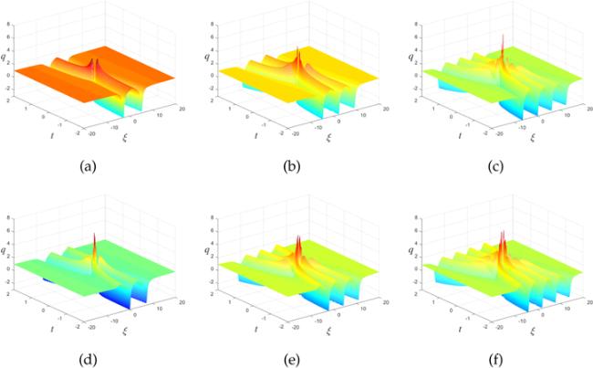
Figure 3. The upper ones are the odd-order rational traveling waves and the lower ones are the even-order rational waves for equation (1), where $\xi $ is a new variable about $x$ and $t,$ $\xi =x+6t.$
From the soliton solution, we can see that when $t$ is large, the higher order soliton will split into some single solitons, but as to the rational traveling wave, we can not receive a similar result from the figures and the exact expression in (37) up to now. Thus we only give the asymptotic expression about the soliton solutions. With the exact soliton solution in equation (35), if the soliton moves along the characteristic curves
$\begin{eqnarray}x=s+4t\pm \displaystyle \frac{1}{2}\,\mathrm{log}(| t| ),\end{eqnarray}$
then the soliton solutions will not approach to zero, otherwise, it will vanish. Substitute this characteristic curves into equation (35) and let $| t| \to \infty ,$ then we can get the asymptotic soliton solutions,
$\begin{eqnarray}\begin{array}{l}\begin{array}{l}{q}_{s}^{[2]}\to 2{\rm{{\rm{sech}} }}\left(2\left(x-4t+\displaystyle \frac{1}{2}\,\mathrm{log}(t)\right)+5\,\mathrm{log}(2)\right)\\ \,-2{\rm{{\rm{sech}} }}\left(2\left(x-4t-\displaystyle \frac{1}{2}\,\mathrm{log}(t)\right)-5\,\mathrm{log}(2)\right),\,t\to +\infty ,\end{array}\\ \begin{array}{l}{q}_{s}^{[2]}\to 2{\rm{{\rm{sech}} }}\left(2\left(x-4t-\displaystyle \frac{1}{2}\,\mathrm{log}(-t)\right)-5\,\mathrm{log}(2)\right)\\ \,-2{\rm{{\rm{sech}} }}\left(2\left(x-4t+\displaystyle \frac{1}{2}\,\mathrm{log}(-t)\right)+5\,\mathrm{log}(2)\right),\,t\to -\infty .\end{array}\end{array}\end{eqnarray}$
When $N=2,$ we know the characteristic curves can be set as
$\begin{eqnarray}x=s+4t+\displaystyle \frac{1-2j}{2}\,\mathrm{log}(| t| ),\,j=-1,0,1,2,\end{eqnarray}$
and its asymptotic expression is
$\begin{eqnarray}\begin{array}{ll}{q}_{s}^{[4]} & \to \,2{\rm{{\rm{sech}} }}\left(2\left(x-4t+\displaystyle \frac{3}{2}\,\mathrm{log}(t)\right)+\,\mathrm{log}\left(\displaystyle \frac{{2}^{16}}{3}\right)\right)\\ & \,-2{\rm{{\rm{sech}} }}\left(2\left(x-4t-\displaystyle \frac{3}{2}\,\mathrm{log}(t)\right)-\,\mathrm{log}\left(\displaystyle \frac{{2}^{16}}{3}\right)\right)\\ & +2{\rm{{\rm{sech}} }}\left(2\left(x-4t-\displaystyle \frac{1}{2}\,\mathrm{log}(t)\right)-4\,\mathrm{log}(2)\right)\\ & \,-2{\rm{{\rm{sech}} }}\left(2\left(x-4t+\displaystyle \frac{1}{2}\,\mathrm{log}(t)\right)+4\,\mathrm{log}(2)\right),\\ & t\to +\infty ,\\ {q}_{s}^{[4]} & \to \,2{\rm{{\rm{sech}} }}\left(2\left(x-4t-\displaystyle \frac{3}{2}\,\mathrm{log}(-t)\right)-\,\mathrm{log}\left(\displaystyle \frac{{2}^{16}}{3}\right)\right)\\ & \,-2{\rm{{\rm{sech}} }}\left(2\left(x-4t+\displaystyle \frac{3}{2}\,\mathrm{log}(-t)\right)+\,\mathrm{log}\left(\displaystyle \frac{{2}^{16}}{3}\right)\right)\\ & +2{\rm{{\rm{sech}} }}\left(2\left(x-4t+\displaystyle \frac{1}{2}\,\mathrm{log}(-t)\right)+4\,\mathrm{log}(2)\right)\\ & \,-2{\rm{{\rm{sech}} }}\left(2\left(x-4t-\displaystyle \frac{1}{2}\,\mathrm{log}(-t)\right)-4\,\mathrm{log}(2)\right),\\ & t\to -\infty .\end{array}\end{eqnarray}$

Following this rule of characteristic curves, for a general $2N$-order soliton, the characteristic curves can be set as

$x=s+4t+\displaystyle \frac{1-2j}{2}\,\mathrm{log}(| t| ),\,j=-N-1,\cdots ,0,1,\cdots ,N.$
As to this result, we only give some comparison graphs between the exact solutions and the asymptotic solution for $t$ positive, the negative one can be given similarly, which is shown in figure 4.
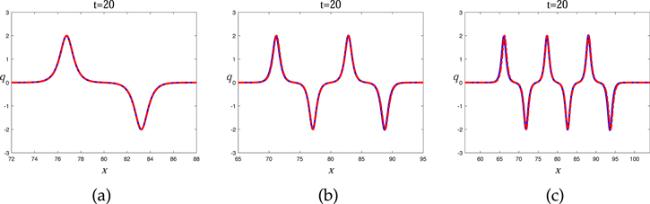
Figure 4. (a)–(c) The comparison between the exact soliton solution and the asymptotic solution, when the corresponding order is second, fourth and sixth respectively. The blue solid line is the exact soliton, and the red dotted line is the asymptotic soliton.

4. Discussions and conclusions

In this paper, we construct two types of solutions to the mKdV equation, one is under the zero background condition and the other one is under the nonzero constant background. It is well known that the zero background soliton can be found for many integrable systems, such as the classical NLS equation. But the nonzero background soliton is very special, especially, in this paper, by choosing one fixed spectral parameter, we get the rational traveling waves. Although this type of solution is rational, it is very different from the well known rogue wave. Its shape is similar to the soliton, which is not a localized solution at the $(x,t)$-direction, which is very interesting. More importantly, the soliton solutions and the rational traveling waves are constructed under the framework of Riemann–Hilbert method, which can be used to discuss some asymptotic behaviors. In [69], the authors discuss the far filed and the near field asymptotics to the higher order soliton and the higher order rogue waves for the NLS equation. Comparing to the NLS equation, the phase term about the mKdV equation becomes more complex, which give a new challenge for study the asymptotics. After this paper, we will try to analyze this asymptotics and hope to get more interesting phenomena.

This work was supported by the Natural Science Foundation of Shandong Province (Grant No. ZR2019QD018), National Natural Science Foundation of China (Grant Nos. 11975143, 12105161, 61602188), CAS Key Laboratory of Science and Technology on Operational Oceanography (Grant No. OOST2021-05), Scientific Research Foundation of Shandong University of Science and Technology for Recruited Talents (Grant Nos. 2017RCJJ068, 2017RCJJ069).

1
Ablowitz M J Kaup D J Newell A C Segur H 1974 The inverse scattering transform-Fourier analysis for nonlinear problems Stud. Appl. Math. 53 249

DOI

2
Ablowitz M J Segur H 1981 Solitons and the Inverse Scattering Transform Philadelphia, PA Society for Industrial and Applied Mathematics

3
Belokolos E D Bobenko A I Enolskii V Z Its A R Matveev V B 1994 Algebro-Geometric Approach to Nonlinear Integrable Equations Berlin Springer

4
Zakharov V E Shabat A B 1972 Exact theory of two-dimensional self-focusing and one-dimensional self-modulation of waves in nonlinear media Sov. Phys. JETP 34 62

5
Bilman D Miller P D 2019 A robust inverse scattering transform for the focusing nonlinear Schrödinger equation Commun. Pure Appl. Math. 72 1722

DOI

6
Bilman D Ling L L Miller P D 2020 Extreme superposition: rogue waves of infinite order and the Painlevé-III hierarchy Duke Math. J. 169 671

DOI

7
Bilman D. Miller P. D. 2021 Extreme superposition: high-order fundamental rogue waves in the far-field regime arXiv:2103.00337

8
Bilman D Buckingham R 2019 Large-order asymptotics for multiple-pole solitons of the focusing nonlinear Schrödinger equation J. Nonlinear Sci. 29 2185

DOI

9
Bilman D Buckingham R Wang D S 2021 Far-field asymptotics for multiple-pole solitons in the large-order limit J. Differ. Equ. 297 320

DOI

10
Chen S Y Yan Z Y 2019 The Hirota equation: Darboux transform of the Riemann-Hilbert problem and higher-order rogue waves Appl. Math. Lett. 95 65

DOI

11
Chen S Y Yan Z Y 2019 The higher-order nonlinear Schrödinger equation with non-zero boundary conditions: robust inverse scattering transform, breathers, and rogons Phys. Lett. A 383 125906

DOI

12
Peng W. Q. Chen Y. 2021 Soliton solutions for nonlocal Hirota equation with non-zero boundary conditions using Riemann-Hilbert method and PINN algorithm Physica D 435 133274

13
Zhang X E Chen Y 2019 Inverse scattering transformation for generalized nonlinear Schrödinger equation Appl. Math. Lett. 98 306

DOI

14
Chen Y R Feng B F Ling L L 2021 The robust inverse scattering method for focusing Ablowitz-Ladik equation on the non-vanishing background Physica D 424 132954

DOI

Outlines

/