


1. Introduction
Researchers have taken great attention to study nonlinear phenomena. Nonlinear partial differential equations (NPDEs) appear in applied mathematics and engineering research areas with various applications. Several goals of applied mathematics are presented to identify and explain exact solutions for NPDEs [1–8]. Numerous NPDEs such as the Sawada–Kotera equation [9–11], the Gilson–Pickering model [12, 13], the Fokas–Lenells model [14–16], the Hirota equation [17, 18], the Sasa–Satsuma equation [19–21], and others [22–31] have been discussed and analyzed in different branches of science
The perturbed CLL model is given by [32]:1 ) is studied when $m=1$
$\begin{eqnarray}\begin{array}{l}{\rm{i}}{\psi }_{t}+\alpha {\psi }_{xx}+{\rm{i}}\beta {\left|\psi \right|}^{2}{\psi }_{x}={\rm{i}}\left[\gamma {\psi }_{x}+\mu {(| \psi {| }^{2m}\psi )}_{x}\right.\\ \left.+\delta {(| \psi {| }^{2m})}_{x}\psi \right],\end{array}\end{eqnarray}$
where $\gamma $ is the inter-modal dispersion coefficient, $\mu $ symbolizes the coefficient of self-steepening for short pulses, and $\delta $ is the coefficient of nonlinear dispersion. Additionally, $\alpha $ is the coefficient of the velocity dispersion and $\beta $ is the coefficient of nonlinearity. Here, equation ( $\begin{eqnarray}{\rm{i}}{\psi }_{t}+\alpha {\psi }_{xx}+{\rm{i}}\beta {\left|\psi \right|}^{2}{\psi }_{x}={\rm{i}}\left[\gamma {\psi }_{x}+\mu {(| \psi {| }^{2}\psi )}_{x}+\delta {(| \psi {| }^{2})}_{x}\psi \right].\end{eqnarray}$
The main object of this article is to study and analyze equation (2 ) by finding a variety of solutions via the GERFM for the perturbed CLL model that represents the propagation of an optical pulse in plasma and optical fiber. Recently, the field of applications of this equation has become an important part of plasma physics. Previously this equation has been investigated by many researchers. Houwe et al [33] show the chirped and the corresponding chirp with their stability for the CLL model. Biswas has obtained soliton solutions by using semi-inverse variational principle [34]. Akinyemi and others studied the CLL model with the help of the Jacobi elliptic functions [35]. Kudryashov found general solutions by using different methods with the elliptic function approach [36]. Apart from this, the Sardar subequation technique was utilized to obtain solitary wave solutions for this equation [37], and numerous studies have been done for the CLL model [38–40]. In this study, we examine this model via the generalized exponential rational function method (GERFM). This method is presented by Ghanbari and others to study different partial differential equations [41, 42]. Furthermore, Ghanbari and Aguilar used this approach to find some novel solutions of the Radhakrishnan–Kundu–Lakshmanan equation with $\beta $-conformable time derivative [43].
This study is organized as follows; introduction is given in section 1 . In section 2 , we focused on presenting the GERFM. In section 3 , we established and studied a variety of exact solutions for the perturbed CLL model by applying the GERFM. The conclusion and the physical interpretations of this study are presented in section 4 .
2. Outline of GERFM
In this section, the GERFM is explained in the following manner:
Step 1: Consider the general form of a nonlinear partial differential as:3 ) becomes a nonlinear ordinary differential equation with the use of equation (4 ) and written as:
$\begin{eqnarray}Q(\psi ,{\psi }_{x},{\psi }_{t},{\psi }_{xx},{\psi }_{tt},{\psi }_{tx},\cdots )=0,\end{eqnarray}$
where $Q$ is a polynomial function in $\psi (x,t)$ and its partial derivatives. Suppose that the wave transformation takes the form: $\begin{eqnarray}\psi (x,t)=P(\eta ){\,{\rm{e}}}^{{\rm{i}}(-kx+wt+\theta )},\eta =x-ht,\end{eqnarray}$
where $P(\eta )$ is the amplitude, $k$ is the wave number, $w$ is the frequency, $\theta $ is the phase constant, and $x-ht$ is the traveling coordinate. Equation ( $\begin{eqnarray}\phi ({P}^{{\prime} },{P}^{{\prime\prime} },P^{\prime\prime \prime} ,\cdots )=0.\end{eqnarray}$
Step 2: The solitary wave solutions of equation (5 ) have the form:
$\begin{eqnarray}P(\eta )={A}_{0}+\displaystyle \sum _{K=1}^{n}{A}_{K}\varphi {\left(\eta \right)}^{K}+\displaystyle \sum _{K=1}^{n}{B}_{K}\varphi {\left(\eta \right)}^{-K},\end{eqnarray}$
where $\begin{eqnarray}\varphi (\eta )=\displaystyle \frac{{r}_{1}{{\rm{e}}}^{{s}_{1}\eta }+{r}_{2}{{\rm{e}}}^{{s}_{2}\eta }}{{r}_{3}{{\rm{e}}}^{{s}_{3}\eta }+{r}_{4}{{\rm{e}}}^{{s}_{4}\eta }},\end{eqnarray}$
here ${r}_{n},$ ${s}_{n}$ $\left(1\leqslant n\leqslant 4\right)$ are real $/\,$complex constants, ${A}_{0},$ ${A}_{K},$ ${B}_{K}$ are constants to be determined, and $n$ will be determined by the known balance principle.Step 3: Substituting equation (6 ) into equation (5 ), we get a system of polynomials in $\varphi \left(\eta \right).$ By equating the same order terms, we obtain an algebraic system of equations. By using any suitable computer software, we solve this system and determine the values of ${A}_{0},$ ${A}_{K},$ ${B}_{K}.$ Thus, we can easily obtain non-trivial exact solutions of equation (5 ).
Step 4: Putting non-trivial solutions obtained from Step 3 into (6 ), we attain the exact soliton solutions of equation (2 ).
3. Applications
In this portion, we apply the GERFM to equation (2 ). Firstly, inserting equation (4 ) into equation (2 ) yields8 ) is given by
$\begin{eqnarray}\begin{array}{c}-{\rm{i}}h{P}^{{\rm{{\prime} }}}-wP+\alpha {P}^{{\rm{{\prime} }}{\rm{{\prime} }}}-2k\alpha {\rm{i}}{P}^{{\rm{{\prime} }}}-\alpha {k}^{2}P+{\rm{i}}\beta {P}^{2}{P}^{{\rm{{\prime} }}}\\ +\beta k{P}^{3}-{\rm{i}}\gamma {P}^{{\rm{{\prime} }}}-\gamma kP-3{\rm{i}}\mu {P}^{2}{P}^{{\rm{{\prime} }}}-\mu k{P}^{3}-2{\rm{i}}\delta {P}^{2}{P}^{{\rm{{\prime} }}}=0.\end{array}\end{eqnarray}$
The real part of equation ( $\begin{eqnarray}\left(-w-\alpha {k}^{2}-\gamma k\right)P+\alpha {P}^{{\rm{{\prime} }}{\rm{{\prime} }}}+k\left(\beta -\mu \right){P}^{3}=0,\end{eqnarray}$
and the imaginary part has the form $\begin{eqnarray}\left(-h-2k\alpha -\gamma \right){P}^{{\prime} }+\left(\beta -3\mu -2\delta \right){P}^{2}{P}^{{\prime} }=0.\end{eqnarray}$
Set the coefficients of the components of the imaginary part equal zero, we get $h=-2k\alpha -\gamma ,$ and $\beta =3\mu +2\delta .$ Considering these constraints in equation (9 ), we get
$\begin{eqnarray}\left(-w-\alpha {k}^{2}-\gamma k\right)P+\alpha {P}^{{\rm{{\prime} }}{\rm{{\prime} }}}+2k\left(\delta +\mu \right){P}^{3}=0.\end{eqnarray}$
By using the balance principle, we get $n=1.$ Also, we use $r=\left[{r}_{1},{r}_{2},{r}_{3},{r}_{4}\right]$ and $s=\left[{s}_{1},{s}_{2},{s}_{3},{s}_{4}\right]$ notation. Considering equations (6 ) and (7 ), we may express the solution of equation (11 ) as follow:
$\begin{eqnarray}P(\eta )={A}_{0}+{A}_{1}\varphi (\eta )+{B}_{1}\displaystyle \frac{1}{\varphi (\eta )}.\end{eqnarray}$
Family 1: For $r=\left[-2,-1,1,1\right],$ $s=\left[0,1,0,1\right],$ we get
$\begin{eqnarray}\varphi (\eta )=\displaystyle \frac{-2-{{\rm{e}}}^{\eta }}{1+{{\rm{e}}}^{\eta }}.\end{eqnarray}$
Case 1: When ${B}_{1}=0,$ $\gamma =\tfrac{-w}{k}+\tfrac{1}{2}{{A}_{1}}^{2}\left(1+2{k}^{2}\right)\left(\delta +\mu \right),$ ${A}_{0}=\tfrac{3{A}_{1}}{2},$ $\alpha =-{{A}_{1}}^{2}k\left(\delta +\mu \right).$
Taking into account equations (12 ) and (13 ) and by direct substitution in equation (4 ), we get
$\begin{eqnarray*}{\psi }_{1}(x,t)=\left(\displaystyle \frac{3{A}_{1}}{2}+{A}_{1}\left(\displaystyle \frac{-2-{{\rm{e}}}^{x-ht}}{1+{{\rm{e}}}^{x-ht}}\right)\right){{\rm{e}}}^{{\rm{i}}(-kx+wt+\theta )}.\end{eqnarray*}$
Considering $h=-2k\alpha -\gamma ,$ the exact solution of equation (2 ) reads
$\begin{eqnarray}\begin{array}{l}{\psi }_{1}(x,t)\\ \,=\,{{\rm{e}}}^{{\rm{i}}\left(-kx+wt+\theta \right)}\left(\displaystyle \frac{3{A}_{1}}{2}+\displaystyle \frac{{A}_{1}\left(-2-{{\rm{e}}}^{x-t\left(\displaystyle \frac{w}{k}+2{{A}_{1}}^{2}{k}^{2}\left(\delta +\mu \right)-\displaystyle \frac{1}{2}{{A}_{1}}^{2}\left(1+2{k}^{2}\right)\left(\delta +\mu \right)\right)}\right)}{1+{{\rm{e}}}^{x-t\left(\displaystyle \frac{w}{k}+2{{A}_{1}}^{2}{k}^{2}\left(\delta +\mu \right)-\displaystyle \frac{1}{2}{{A}_{1}}^{2}\left(1+2{k}^{2}\right)\left(\delta +\mu \right)\right)}}\right).\end{array}\end{eqnarray}$
This is corresponding to optical exponential solutions.
Case 2: When ${A}_{1}=0,$ ${A}_{0}=\tfrac{3{B}_{1}}{4},$ $\alpha =-\tfrac{1}{4}{B}_{1}^{2}k\left(\delta +\mu \right),$ and $\gamma =-\tfrac{w}{k}+\tfrac{1}{8}{B}_{1}^{2}\left(1+2{k}^{2}\right)\left(\delta +\mu \right).$
Taking into account equation (12 ), equation (13 ) and the above values in equation (4 ), we get
$\begin{eqnarray*}{\psi }_{2}(x,t)=\left(\displaystyle \frac{3{B}_{1}}{4}+\displaystyle \frac{{B}_{1}\left(1+{{\rm{e}}}^{x-ht}\right)}{-2-{{\rm{e}}}^{x-ht}}\right){{\rm{e}}}^{{\rm{i}}(-kx+wt+\theta )}.\end{eqnarray*}$
Considering $h=-2k\alpha -\gamma $ yields the exact solution of equation (2 ) as
$\begin{eqnarray}\begin{array}{l}{\psi }_{2}(x,t)\\ \,=\,\left(\displaystyle \frac{3{B}_{1}}{4}+\displaystyle \frac{{B}_{1}\left(1+{{\rm{e}}}^{x-t\left(\displaystyle \frac{w}{k}+\displaystyle \frac{1}{2}{B}_{1}^{2}{k}^{2}\left(\delta +\mu \right)-\displaystyle \frac{1}{8}{B}_{1}^{2}\left(1+2{k}^{2}\right)\left(\delta +\mu \right)\right)}\right)}{-2-{{\rm{e}}}^{x-t\left(\displaystyle \frac{w}{k}+\displaystyle \frac{1}{2}{B}_{1}^{2}{k}^{2}\left(\delta +\mu \right)-\displaystyle \frac{1}{8}{B}_{1}^{2}\left(1+2{k}^{2}\right)\left(\delta +\mu \right)\right)}}\right){{\rm{e}}}^{{\rm{i}}(-kx+wt+\theta )}.\end{array}\end{eqnarray}$
Equation (15 ) represents optical exponential solutions.
Family 2: For this group, we take $r=[-2-{\rm{i}},2-{\rm{i}},-1,1],$ $s=[{\rm{i}},-{\rm{i}},{\rm{i}},-{\rm{i}}],$ we get
$\begin{eqnarray}\varphi (\eta )=\displaystyle \frac{\cos (\eta )+2\,\sin (\eta )}{\sin (\eta )}.\end{eqnarray}$
Case 1: When ${A}_{0}=\mp \tfrac{2\sqrt{\alpha }}{\sqrt{-k\left(\delta +\mu \right)}},$ ${A}_{1}=0,$ ${B}_{1}=\pm \tfrac{5\sqrt{\alpha }}{\sqrt{-k\left(\delta +\mu \right)}},$ and $\gamma =-\tfrac{(w+(-2+{k}^{2})\alpha )}{k}.$
Taking into account equation (12 ), equation (16 ), and these values in equation (4 ), we get
$\begin{eqnarray*}{\psi }_{3}(x,t)=\left(\displaystyle \frac{2\sqrt{\alpha }}{\sqrt{-k\left(\delta +\mu \right)}}-\displaystyle \frac{5\sqrt{\alpha }\,\sin \left(x-ht\right)}{\sqrt{-k\left(\delta +\mu \right)}\left(\cos \left(x-ht\right)+2\,\sin \left(x-ht\right)\right)}\right){{\rm{e}}}^{{\rm{i}}(-kx+wt+\theta )}.\end{eqnarray*}$
Considering $h=-2k\alpha -\gamma ,$ we reach the exact solution of equation (2 ) as
$\begin{eqnarray}\begin{array}{l}{\psi }_{3}(x,t)={{\rm{e}}}^{{\rm{i}}\left(-kx+wt+\eta \right)}\left( \frac{2\sqrt{\alpha }}{\sqrt{-k\left(\delta +\mu \right)}}\right.\\ -\left. \frac{5\sqrt{\alpha }\,\sin \left(x-t\left(-2k\alpha + \frac{w+\left(-2+{k}^{2}\right)\alpha }{k}\right)\right)}{\sqrt{-k\left(\delta +\mu \right)}\left(\cos \left(x-t\left(-2k\alpha + \frac{w+\left(-2+{k}^{2}\right)\alpha }{k}\right)\right)+2\,\sin \left(x-t\left(-2k\alpha + \frac{w+\left(-2+{k}^{2}\right)\alpha }{k}\right)\right)\right)}\right)\end{array}\end{eqnarray}$
This is corresponding to optical trigonometric solutions under conditions $\alpha \gt 0,$ $k\left(\delta +\mu \right)\lt 0.$
Case 2: When ${A}_{0}=\mp \displaystyle \frac{2\sqrt{\alpha }}{\sqrt{-k\left(\delta +\mu \right)}},$ ${A}_{1}=\pm \displaystyle \frac{\sqrt{\alpha }}{\sqrt{-k\left(\delta +\mu \right)}},$ ${B}_{1}=0,$ and $\gamma =-\displaystyle \frac{w+\left(-2+{k}^{2}\right)\alpha }{k}.$
Taking into account equation (12 ), equation (16 ), and these values in equation (4 ), we get
$\begin{eqnarray*}\begin{array}{l}{\psi }_{4}(x,t)\,=\,\left(-\displaystyle \frac{2\sqrt{\alpha }}{\sqrt{-k\left(\delta +\mu \right)}}\right.\\ \left.\,+\,\displaystyle \frac{\sqrt{\alpha }\csc \left(x-ht\right)\left(\cos \left(x-ht\right)+2\,\sin \left(x-ht\right)\right)}{\sqrt{-k\left(\delta +\mu \right)}}\right){{\rm{e}}}^{{\rm{i}}(-kx+wt+\theta )}.\end{array}\end{eqnarray*}$
Considering $h=-2k\alpha -\gamma ,$ we get the exact solution of equation (2 ) as follows
$\begin{eqnarray}\begin{array}{l}{\psi }_{4}(x,t)={{\rm{e}}}^{{\rm{i}}(-kx+wt+\theta )}\left(-\tfrac{2\sqrt{\alpha }}{\sqrt{-k\left(\delta +\mu \right)}}+\right.\\ \left. \frac{\sqrt{\alpha }\csc \left(x-t\left(-2k\alpha +\tfrac{w+\left(-2+{k}^{2}\right)\alpha }{k}\right)\right)\left(\cos \left(x-t\left(-2k\alpha +\tfrac{w+\left(-2+{k}^{2}\right)\alpha }{k}\right)\right)+2\,\sin \left(x-t\left(-2k\alpha +\tfrac{w+\left(-2+{k}^{2}\right)\alpha }{k}\right)\right)\right)}{\sqrt{-k\left(\delta +\mu \right)}}\right).\end{array}\end{eqnarray}$
Equation (18 ) is corresponding to the optical trigonometric solutions under conditions $\alpha \gt 0,$ $k\left(\delta +\mu \right)\lt 0.$
Family 3: In this group $r=[2,0,1,1],$ $s=[-1,0,1,-1],$ we get
$\begin{eqnarray}\varphi (\eta )=\displaystyle \frac{\cosh (\eta )-\,\sinh (\eta )}{\cosh (\eta )}.\end{eqnarray}$
Case 1: When ${A}_{0}=\mp \displaystyle \frac{\sqrt{\alpha }}{\sqrt{-k\left(\delta +\mu \right)}},$ ${A}_{1}=\pm \displaystyle \frac{\sqrt{\alpha }}{\sqrt{-k\left(\delta +\mu \right)}},$ ${B}_{1}=0,$ and $\gamma =-\displaystyle \frac{(w+(-2+{k}^{2})\alpha )}{k}.$
Taking into account equation (12 ), equation (19 ), and these values in equation (4 ), we obtain
$\begin{eqnarray*}\begin{array}{l}{\psi }_{5}(x,t)=\left(-\tfrac{\sqrt{\alpha }}{\sqrt{-k\left(\delta +\mu \right)}}+\right.\\ \left.\displaystyle \frac{\sqrt{\alpha }{\rm{sech}} (x-ht)\left(\cosh (x-ht)-\,\sinh (x-ht)\right)}{\sqrt{-k\left(\delta +\mu \right)}}\right){{\rm{e}}}^{{\rm{i}}(-kx+wt+\theta )}.\end{array}\end{eqnarray*}$
Considering $h=-2k\alpha -\gamma ,$ we get the exact solution of equation (2 ) as follows
$\begin{eqnarray}\begin{array}{l}{\psi }_{5}(x,t)={{\rm{e}}}^{{\rm{i}}(-kx+wt+\theta )}\left(-\tfrac{\sqrt{\alpha }}{\sqrt{-k\left(\delta +\mu \right)}}+\right.\\ \left. \frac{\sqrt{\alpha }\,{\rm{sech}} \left(x-t\left(-2k\alpha +\tfrac{w+\left(2+{k}^{2}\right)\alpha }{k}\right)\right)\left(\cosh \left(x-t\left(-2k\alpha +\tfrac{w+\left(2+{k}^{2}\right)\alpha }{k}\right)\right)-\,\sinh \left(x-t\left(-2k\alpha +\tfrac{w+\left(2+{k}^{2}\right)\alpha }{k}\right)\right)\right)}{\sqrt{-k\left(\delta +\mu \right)}}\right).\end{array}\end{eqnarray}$
This is corresponding to the optical hyperbolic solutions under conditions $\alpha \gt 0,$ $k\left(\delta +\mu \right)\lt 0.$
Family 4: For $r=[-1,1,1,1],$ $s=[1,-1,1,-1],$ we get
$\begin{eqnarray}\varphi (\eta )=\displaystyle \frac{-\,\sinh (\eta )}{\cosh (\eta )}.\end{eqnarray}$
Case 1: When ${A}_{0}=0,$ ${A}_{1}=0,$ ${B}_{1}=\mp \displaystyle \frac{\sqrt{\alpha }}{\sqrt{-k\left(\delta +\mu \right)}},$ and $\gamma =-\displaystyle \frac{(w+(-2+{k}^{2})\alpha )}{k},$ and $\gamma =-\displaystyle \frac{w+\left(2+{k}^{2}\right){\rm{\alpha }}}{k}.$
Taking into account equation (12 ), equation (21 ), and these values in equation (4 ), we have
$\begin{eqnarray*}{\psi }_{6}(x,t)=\left(\displaystyle \frac{\sqrt{\alpha }\,\coth (x-ht)}{\sqrt{-k\left(\delta +\mu \right)}}\right){{\rm{e}}}^{{\rm{i}}(-kx+wt+\theta )}.\end{eqnarray*}$
Considering $h=-2k\alpha -\gamma ,$ the exact solution of equation (2 ) takes the form
$\begin{eqnarray}{\psi }_{6}(x,t)=\left(\displaystyle \frac{\sqrt{\alpha }\,\coth \left(x-t\left(-2k\alpha +\tfrac{w+\left(2+{k}^{2}\right)\alpha }{k}\right)\right)}{\sqrt{-k\left(\delta +\mu \right)}}\right){{\rm{e}}}^{{\rm{i}}(-kx+wt+\theta )}.\end{eqnarray}$
This is corresponding to the optical singular soliton solutions under conditions $\alpha \gt 0,$ $k\left(\delta +\mu \right)\lt 0.$
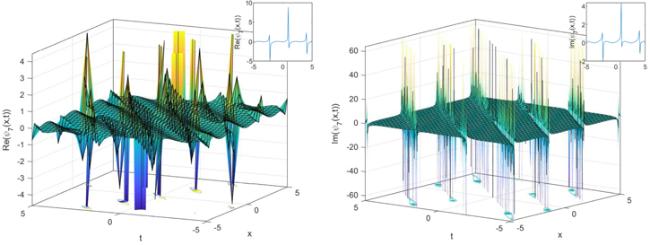
In figure (4), the amplitude of the solution given is very high in the medium through which the wave is propagated, thus this singular periodic wave is a shock wave.
Family 5: Using $r=[{\rm{i}},-{\rm{i}},1,1],$ $s=[{\rm{i}},-{\rm{i}},{\rm{i}},-{\rm{i}}],$ we get
$\begin{eqnarray}\varphi (\eta )=\displaystyle \frac{-\,\sin (\eta )}{\cos (\eta )}.\end{eqnarray}$
Case 1: When ${A}_{0}=0,$ ${A}_{1}=\mp \tfrac{\sqrt{\alpha }}{\sqrt{-k\left(\delta +\mu \right)}},$ ${B}_{1}=\pm \tfrac{\sqrt{\alpha }}{\sqrt{-k\left(\delta +\mu \right)}},$ and $\gamma =-\tfrac{w+\left(-8+{k}^{2}\right)\alpha }{k}.$
Taking into account equation (12 ), equation (23 ), and these values in equation (4 ), we obtain
${\psi }_{7}(x,t)=\left(\displaystyle \frac{\sqrt{\alpha }\,\cot \left(x\,-\,ht\right)}{\sqrt{-k\left(\delta +\mu \right)}}-\displaystyle \frac{\sqrt{\alpha }\,\tan (x-ht)}{\sqrt{-k\left(\delta +\mu \right)}}\right){{\rm{e}}}^{{\rm{i}}(-kx+wt+\theta )}.$
Considering $h=-2k\alpha -\gamma ,$ the exact solution of equation (2 ) takes the form
$\begin{eqnarray}\begin{array}{c}{\psi }_{7}(x,t)=\left(\displaystyle \frac{\sqrt{\alpha }\,\cot \left(x-t\left(-2k\alpha +\tfrac{w+\left(-8+{k}^{2}\right)\alpha }{k}\right)\right)}{\sqrt{-k\left(\delta +\mu \right)}}-\right.\\ \left.\displaystyle \frac{\sqrt{\alpha }\,\tan \left(x-t\left(-2k\alpha +\tfrac{w+\left(-8+{k}^{2}\right)\alpha }{k}\right)\right)}{\sqrt{-k\left(\delta +\mu \right)}}\right){{\rm{e}}}^{{\rm{i}}(-kx+wt+\theta )}.\end{array}\end{eqnarray}$
This is corresponding to the optical periodic soliton solutions under conditions $\alpha \gt 0,$ $k\left(\delta +\mu \right)\lt 0.$
Case 2: When ${A}_{0}=0,$ ${A}_{1}=0,$ ${B}_{1}=\mp \displaystyle \frac{\sqrt{\alpha }}{\sqrt{-k(\delta +\mu )}},$ and $\gamma =-\displaystyle \frac{w+\left(-2+{k}^{2}\right)\alpha }{k}.$
Taking into account equation (12 ), equation (23 ) and these values in equation (4 ), we get
$\begin{eqnarray*}{\psi }_{8}(x,t)=\left(-\displaystyle \frac{\sqrt{\alpha }\,\cot \left(x-ht\right)}{\sqrt{-k\left(\delta +\mu \right)}}\right){{\rm{e}}}^{{\rm{i}}(-kx+wt+\theta )}.\end{eqnarray*}$
Considering $h=-2k\alpha -\gamma ,$ the exact solution of equation (2 ) is given by
$\begin{eqnarray}{\psi }_{8}(x,t)=\left(-\displaystyle \frac{\sqrt{\alpha }\,\cot \left[x-t\left(-2k\alpha +\tfrac{w+\left(-2+{k}^{2}\right)\alpha }{k}\right)\right]}{\sqrt{-k\left(\delta +\mu \right)}}\right){{\rm{e}}}^{{\rm{i}}(-kx+wt+\theta )}.\end{eqnarray}$
Equation (25 ) is corresponding to the optical periodic soliton solutions under conditions $\alpha \gt 0,$ $k\left(\delta +\mu \right)\lt 0.$
4. Conclusion
Herein, we have divided our results into two main parts as follows:
4.1. Overview
The current work recovered a variety of optical soliton solutions with different wave structures for the perturbed CLL model is obtained via the GERFM. According to the suitable choice of the self-steepening short pulses $\mu $ and the nonlinear dispersion coefficient $\delta ,$ the obtained solutions are classified into optical singular, periodic, hyperbolic, exponential, and trigonometric soliton solutions. Furthermore, the physical meaning of these solutions is graphically investigated through 2D- and 3D- plots. To the best of our knowledge, these results were obtained for the first time for this model. This kind of study is helpful for a physician in planning and decision-making for the treatment of optical pulse in plasma and optical fibers.
4.2. The physical interpretation
In figures 1–5, as changing the values of $\mu $ and $\delta ,$ the rise steepening of the wave will change. For different values of the parameter $\alpha ,$ as an example, the velocity distribution of the wave will be changed as seen in figure 3. In figure 4, when the value of $w$ is increased, the wavelength is decreased. This feature is also observed in figures 1–5. In summary, the obtained solutions are classified into the following categories: equations (14 ) and (15 ) represent optical exponential solutions, equations (17 ) and (18 ) investigate optical trigonometric solutions, equation (20 ) represents an optical hyperbolic solutions, equation (22 ) shows an optical singular soliton solution, and finally equations (24 ) and (25 ) introduce optical periodic soliton solutions.
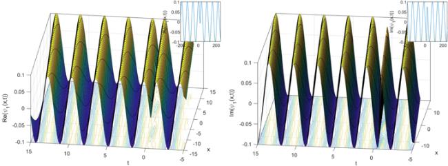
Figure 1. Optical exponential solutions of equation ( |
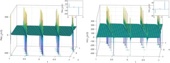
Figure 2. Optical trigonometric solutions of equation ( |
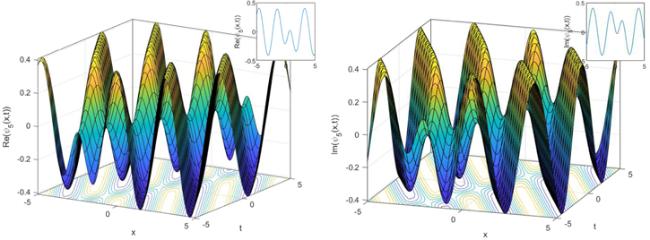
Figure 3. Optical hyperbolic solutions of equation ( |
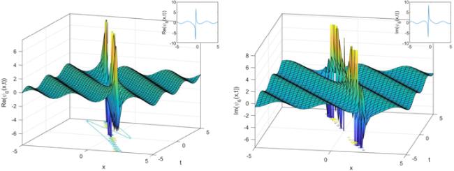
Figure 4 Optical singular soliton solutions of equation ( |
Figure 5. Optical periodic soliton solutions of equation ( |