


1. Introduction
The nonlinear soliton equation is an important part of the field of mathematical physics, which is used to describe the state or process changing with time in physics, mechanics or other natural sciences [1, 2]. As the carrier of soliton theory, the development of the nonlinear equation has always been the focus of mathematical physics researchers.
With the development of computer computing ability, the deep learning method has made great progress in the field of mathematical physics. In recent years, a deep learning numerical method has been developed to solve many problems related to nonlinear evolution equations. The deep learning method approximates potential solutions by using the neural network, which is usually more effective than ordinary numerical methods [3, 4]. In 2017, Raissi et al [3] proposed the physics-informed neural networks(PINNs) to solve partial differential equations, such neural networks are constrained to respect any symmetries, invariances, or conservation principles. Han et al [5] reconstructed partial differential equations from backward stochastic differential equations, and used neural networks to approximate the gradient of unknown solutions to solve general high-dimensional parabolic partial differential equations. In 2018, Justin et al [6] used DGM (depth Galerkin method) to study the numerical driven solution of high-dimensional partial differential equations. In 2020, Chen and his group used the PINNs to solve localized wave solutions of second and third order nonlinear equations such as the KdV equation, the Burgers equation [7, 8]. In 2021, Marcucci et al [9] studied theoretically artificial neural networks with a nonlinear wave as a reservoir layer and developed a new computing model driven by nonlinear partial differential equations. In 2021, Chen and his group proposed a new residual neural network to solve the sine-Gordon equation [10]. In 2021, Wang and Yan [11] studied the numerical driven solution of the defocused NLS equation by using the PINNs. In 2021, Li and his group solved the forward and inverse problems of the NLS equation with the generalized ${\mathscr{P}}{\mathscr{T}}$-symmetric Scarf-2 potential [12]. In 2021, Chen and his group proposed an improved deep learning method to recover the solitons, breathers and rogue wave solutions of the NLS equation, and used physical constraints to analyze the error for the first time [13]. In 2021, Chen and his group improved the PINNs method by introducing the neuron-wise locally adaptive activation function [14, 15]. In 2021, Chen and his group used the PINNs to research the data-driven rogue periodic wave, breather wave, soliton wave and periodic wave solutions of the Chen–Lee–Liu equation, which is the first time to solve the data-driven rogue periodic wave [16]. In 2022, Li and his group used the gradient-optimized PINNs (GOPINNs) deep learning method to obtain the data-driven rational wave solution and soliton molecules solution for the complex modified KdV equation [17]. In 2022, Chen and his group proposed a two-stage PINN method based on conserved quantity. Compared with the original method, this method can significantly improve the prediction accuracy [18]. This is significant progress in the research of the PINNs.
At present, the deep learning method is only used to solve low-order nonlinear problems or low-order linear problems, and its applicability to high-order nonlinear problems is undiscovered. We apply the deep learning method and the physics-informed neural networks [3] to solve high-order nonlinear equations and show the efficiency and effectiveness. Specifically, numerical driven solutions of the fourth-order Boussinesq equation and the fifth-order KdV equation are studied.
The KdV equation has always been an important part of nonlinear mathematical and physical model, and it is also a hotspot of numerical methods [27–29]. Some progress has also been made in the study of the numerical solution of the fifth-order KdV equation [30–32]. The numerical driven solution for the KdV equation has been solved by Raissi et al [3] and Li, Chen [8], where Raissi et al used the discrete time model to solve the KdV equation, and Li and Chen used the continuous time model to solve the KdV equation. However, due to the complexity of high-order nonlinear equations, the numerical driven solution of the high-order nonlinear problem has not been solved. We will illustrate the applicability of the deep learning method to fifth-order nonlinear soliton equations by solving the fifth-order KdV equation.
The paper is organized as follows. In section 2 , we will introduce the deep learning method to solve high-order equations. In section 3 , the deep learning method is used to reproduce the one-soliton and the two-soliton numerical driven solution for the fourth-order Boussinesq equation. In the numerical driven solution, we find the dynamic behavior of solitons interaction. Specifically, the numerical driven solution of the chasing-soliton and the collising-soliton for the Boussinesq equation are solved, and the dynamic behavior between solitons is reproduced from the numerical driven solution. In section 4 , the one-soliton and the two-soliton numerical driven solution for the fifth-order KdV equation are obtained. In the numerical driven solution, the dynamic behavior of solitons interaction can be observed. Finally, some concluding discussions and remarks are contained in section 5 .
2. Method
Considering the following form of the (1 + 1)-dimensional fourth-order and fifth-order nonlinear soliton equations
$\begin{eqnarray}\begin{array}{l}{\chi }_{1}({u}_{t},{u}_{tt})={\chi }_{2}(u,{u}_{x},{u}_{xx},{u}_{xxx},{u}_{xxxx},{u}_{xxxxx}),\end{array}\end{eqnarray}$
where the subscripts $t$ and $x$ denote the partial derivatives about time and space, and is a linear function of the time derivative of $u(x,t),$ ${\chi }_{2}$ is a nonlinear function of $u(x,t)$ and its partial derivative to space variable $x.$ Specifically, a multi-layer neural network is built to approximate the potential solution, the automatic differentiation technique is used to obtain its derivatives in time and space.The residual network is defined
$\begin{eqnarray}\begin{array}{l}f={\chi }_{1}({u}_{t},{u}_{tt})-{\chi }_{2}(u,{u}_{x},{u}_{xx},{u}_{xxx},{u}_{xxxx},{u}_{xxxxx}).\end{array}\end{eqnarray}$
The shared parameters of neural networks can be learned by minimizing the loss of mean square error
$\begin{eqnarray}\begin{array}{l}{\rm{L}}{\rm{O}}{\rm{S}}{\rm{S}}={\rm{L}}{\rm{O}}{\rm{S}}{{\rm{S}}}_{u}+{\rm{L}}{\rm{O}}{\rm{S}}{{\rm{S}}}_{f},\end{array}\end{eqnarray}$
$\begin{eqnarray}\begin{array}{l}{\rm{L}}{\rm{O}}{\rm{S}}{{\rm{S}}}_{u}=\displaystyle \frac{1}{{N}_{u}}\displaystyle \sum _{n=1}^{{N}_{u}}| u({x}_{u}^{n},{t}_{u}^{n})-{u}^{n}| ,\\ {\rm{L}}{\rm{O}}{\rm{S}}{{\rm{S}}}_{f}=\displaystyle \frac{1}{{N}_{f}}\displaystyle \sum _{n=1}^{{N}_{f}}| f({x}_{f}^{n},{t}_{f}^{n})| .\end{array}\end{eqnarray}$
${\rm{L}}{\rm{O}}{\rm{S}}{{\rm{S}}}_{u}$ is the mean square error of initial and boundary, ${\rm{L}}{\rm{O}}{\rm{S}}{{\rm{S}}}_{f}$ is the internal calculation error, ${t}_{u}^{n}$ and ${x}_{u}^{n}$ represent the initial and boundary training values, ${t}_{f}^{n}$ and ${x}_{f}^{n}$ are the point collected in $f.$ ${N}_{u}$ is the total number of selected boundary points and initial points, ${N}_{f}$ is the total number of selected internal collection points. A common deep feedforward neural network is used to deal with the high-order nonlinear problems. Figure 1 shows the framework of the physics-informed neural networks. There are activation functions, weights and bias between each layer. The PINNs updates weights and biases by reducing error ${\rm{L}}{\rm{O}}{\rm{S}}{\rm{S}},$ the neural network stops running until the error is lower than the specified standard.
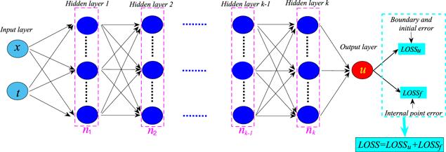
Figure 1. Architecture of the physics-informed neural networks. |
In figure 1, $k$ represents the number of hidden layers, ${n}_{k}$ represents the number of neurons corresponding to the hidden layer. The following aspects of neural networks will be improved to ensure that the PINNs can deal with high-order nonlinear problems. Firstly, we will determine the appropriate number of hidden layers and the corresponding number of neurons. Secondly, the efficiency of the neural network will be improved by optimizing the activation function.
In the process of finding the numerical driven solution of higher-order nonlinear equations, it is important to select the number of hidden layers and neurons in each layer. If the selected neural network structure is not suitable, there will occur over fitting (the deep learning model is superior in training set, but the final result is not good), under fitting (the deep learning model does not capture the characteristics of the data well and cannot solve the equation well), loss of operational efficiency and other problems. Compared with low-order problems, high-order nonlinear problems are more difficult due to the complexity of the equation. Through a large number of experiments, a neural network with four hidden layers is used to deal with high-order nonlinear soliton equations.
On the selection of activation functions, Chen and Li [8] proved that the trigonometric function as the activation function is effective to solve the solitary wave solution of third-order nonlinear soliton equations. In this paper, we will study the deep learning method of high-order nonlinear soliton equations and explore the effectiveness of the trigonometric function as the activation function for high-order nonlinear soliton equations and find the most suitable activation function. In addition, we use the L-BFGS optimization algorithm [33] to set all parameters of the target to minimize the loss function equation (3 ). All numerical examples reported here are run on a Dell computer with Intel Xeon Gold 6320 R processor and 32 GB memory.
3. The numerical driven solution for the Boussinesq equation
Considering the initial problem of the Boussinesq equation
$\begin{eqnarray}\left\{\begin{array}{l}{u}_{tt}-{u}_{xx}-{u}_{xxxx}-3{({u}^{2})}_{xx}=0,\\ u(x,{t}_{0})={u}_{0}(x),\end{array}\right.\end{eqnarray}$
where ${u}_{0}(x)$ is a given real valued smooth function, the subscripts $t$ and $x$ represent partial derivative with respect to time and space respectively.The deep learning method is used to find the one-soliton and the two-soliton numerical driven solution of the equation (5 ) with tanh as the activation function, and the dynamic behavior between solitons is reproduced.
3.1. The one-soliton solution for the Boussinesq equation
In this subsection, the numerical driven one-soliton solution for the Boussinesq equation will be solved. The analytic solution of the one-soliton for the Boussinesq equation can be obtained by using the Hirota method [23, 24]
$\begin{eqnarray}\begin{array}{l}u(x,t)=\displaystyle \frac{{k}_{1}^{2}}{2}{{\rm{sech}} }^{2}\left(\displaystyle \frac{{k}_{1}x+\sqrt{{k}_{1}^{2}+{k}_{1}^{4}}t}{2}+{\xi }_{0}\right).\end{array}\end{eqnarray}$
We could set ${k}_{1}$ = 1, ${\xi }_{0}=0.$ The computation area is truncated in $[-20,20]\times [-5,5]$ for $x$ and $t.$ The corresponding initial condition becomes $\begin{eqnarray}\begin{array}{l}{u}_{0}(x)=\displaystyle \frac{1}{2}{{\rm{sech}} }^{2}\left(\displaystyle \frac{x-5\sqrt{2}}{2}\right).\end{array}\end{eqnarray}$
We generate the data of 201 snapshots directly on regular space-time grid with ${\rm{\Delta }}t$ = 0.05 s. A small training data subset is generated by randomly latin hypercube sampling method [34], the number of collection points is ${N}_{u}$ = 100, ${N}_{f}$ = 20 000. The latent solution $u(x,t)$ can be learned by minimizing the loss function (3 ). The top panel of figure 2 shows the comparison of the predicted spatiotemporal solution and the exact solution. The model achieves a relative ${L}^{2}$ error of size $2.0\times {10}^{-2}$ in a runtime of 152 s and is iterated 170 times to complete the operation. The middle panel of figure 2 shows the absolute error between the exact solution and the predicted solution. The bottom panel of figure 2 shows the detailed comparison of the exact solution and the predicted spatiotemporal solution at different times $t$ = −2.5, $t$ = 0, $t$ = 2.5 respectively. The one-soliton solution for the Boussinesq equation is reconstructed by using the deep learning method accurately. From figure 3, the motion of the reconstructed solitary wave can be clearly observed. The relationship between the number of function evaluations and LOSS is shown in figure 4.
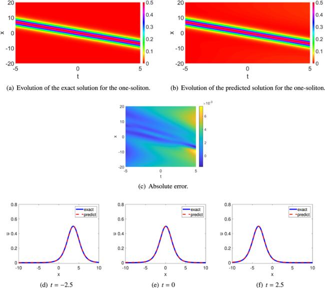
Figure 2. (a), (b) The comparison of the exact solution and the predicted solution for the one-soliton. (c) The absolute error between the exact solution and the predicted solution. (d)–(f) The detailed comparison of the exact solution and the predicted solution at the specific time. |
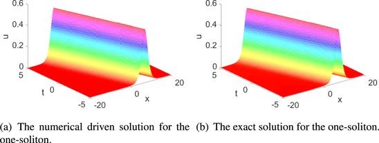
Figure 3. Spatiotemporal evolution of the one-soliton numerical driven solution and the exact solution for the Boussinesq equation. |
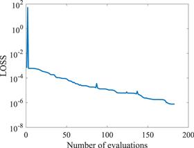
Figure 4. The relationship between the number of function evaluations and LOSS. |
In order to verify the universality of our neural network architecture for the one-soliton solution for the Boussinesq equation, we try to change the value of ${k}_{1}$ and give the numerical solution respectively. The specific results are shown in table 1. The results show that our neural network architecture is effective in solving the one-soliton solution for the Boussinesq equation.
Table 1. The results of the one-soliton solution for the Boussinesq equation calculated by the deep learning method. |
| ${k}_{1}$ | 0.8 | 0.9 | 1.0 | 1.1 | 1.2 | 1.3 | 1.4 |
|---|---|---|---|---|---|---|---|
| ${L}^{2}$ error | $2.79\times {10}^{-2}$ | $3.36\times {10}^{-2}$ | $2.03\times {10}^{-2}$ | $1.9\times {10}^{-2}$ | $1.67\times {10}^{-2}$ | $1.60\times {10}^{-2}$ | $1.62\times {10}^{-2}$ |
| Time (s) | 224 | 191 | 152 | 160 | 294 | 284 | 480 |
| Iterations | 141 | 155 | 170 | 195 | 576 | 416 | 753 |
3.2. The two-soliton solution for the Boussinesq equation
In this subsection, we will calculate the numerical driven two-soliton solution for the Boussinesq equation and reproduce the solitons interaction process. The two-soliton solution for the Boussinesq equation is given [23, 24]
$\begin{eqnarray}\begin{array}{l}u(x,t)\\ \,=2\displaystyle \frac{{k}_{1}^{2}{{\rm{e}}}^{{k}_{1}x+{\omega }_{1}t+{\delta }_{1}}+{k}_{2}^{2}{{\rm{e}}}^{{k}_{2}x+{\omega }_{2}t+{\delta }_{2}}+{({k}_{1}+{k}_{2})}^{2}{{\rm{e}}}^{({k}_{1}+{k}_{2})x+({\omega }_{1}+{\omega }_{2})t+{\delta }_{1}+{\delta }_{2}+{\delta }_{0}}}{1+{{\rm{e}}}^{{k}_{1}x+{\omega }_{1}t+{\delta }_{1}}+{{\rm{e}}}^{{k}_{2}x+{\omega }_{2}t+{\delta }_{2}}+{{\rm{e}}}^{({k}_{1}+{k}_{2})x+({\omega }_{1}+{\omega }_{2})t+{\delta }_{1}+{\delta }_{2}+{\delta }_{0}}}\\ \,-2\displaystyle \frac{{({k}_{1}{{\rm{e}}}^{{k}_{1}x+{\omega }_{1}t+{\delta }_{1}}+{k}_{2}{{\rm{e}}}^{{k}_{2}x+{\omega }_{2}t+{\delta }_{2}}+({k}_{1}+{k}_{2}){{\rm{e}}}^{({k}_{1}+{k}_{2})x+({\omega }_{1}+{\omega }_{2})t+{\delta }_{1}+{\delta }_{2}+{\delta }_{0}})}^{2}}{{(1+{{\rm{e}}}^{{k}_{1}x+{\omega }_{1}t+{\delta }_{1}}+{{\rm{e}}}^{{k}_{2}x+{\omega }_{2}t+{\delta }_{2}}+{{\rm{e}}}^{({k}_{1}+{k}_{2})x+({\omega }_{1}+{\omega }_{2})t+{\delta }_{1}+{\delta }_{2}+{\delta }_{0}})}^{2}},\\ {{\rm{e}}}^{{\delta }_{0}}=-\displaystyle \frac{{({\omega }_{1}-{\omega }_{2})}^{2}-{({k}_{1}-{k}_{2})}^{2}-{({k}_{1}-{k}_{2})}^{4}}{{({\omega }_{1}+{\omega }_{2})}^{2}-{({k}_{1}+{k}_{2})}^{2}-{({k}_{1}+{k}_{2})}^{4}},\end{array}\end{eqnarray}$
where ${\delta }_{1}$ and ${\delta }_{2}$ are constant, ${\omega }_{1}\,$and ${\omega }_{2}$ meet the conditions ${\omega }_{1}^{2}={k}_{1}^{2}+{k}_{1}^{4},$ ${\omega }_{2}^{2}={k}_{2}^{2}+{k}_{2}^{4}$ respectively.The two-soliton solution for the Boussinesq equation has two states, the colliding-soliton and the chasing-soliton. We will find numerical driven solutions of the two forms respectively, and study their dynamic behavior and interaction between solitons.
3.2.1. The colliding-soliton for the Boussinesq equation
We just set ${k}_{1}$ = ${k}_{2}$ = 1.1, ${\delta }_{1}$ = ${\delta }_{2}$ = 0, ${\omega }_{1}\,$and ${\omega }_{2}$ have opposite sign. We generate the data of 201 snapshots directly on regular space-time grid with ${\rm{\Delta }}t$ = 0.05 s. A small training data subset is generated by randomly latin hypercube sampling method [34], the number of collection points is ${N}_{u}$ = 100, ${N}_{f}$ = 25 000. The latent solution $u(x,t)$ is learned by minimizing the loss function (3 ). The top panel of figure 5 shows the comparison of the predicted spatiotemporal solution and the exact solution. The middle panel of figure 5 shows the absolute error between the predicted solution and the exact solution. The bottom panel of figure 5 shows the detailed comparison of the exact solution and the predicted spatiotemporal solution at different time $t$ = −4.5, $t$ = 0, $t$ = 2.5 respectively. The specific spatiotemporal evolution of the colliding-soliton of the Boussinesq equation is given in figure 6. The model achieves a relative ${L}^{2}$ error of size $7.63\times {10}^{-2}$ in a runtime of 430 s. In order to implement the algorithm, the model is iterated 578 times.
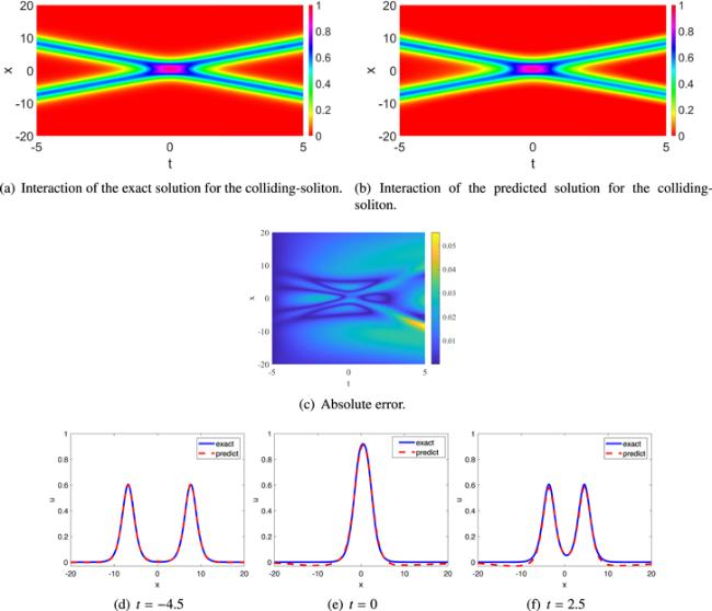
Figure 5. (a), (b) The comparison of the exact solution and the predicted solution for the colliding-soliton. (c) The absolute error between the exact solution and the predicted solution. (d)–(f) The detailed comparison of the exact solution and the predicted spatiotemporal solution at the specific time. |
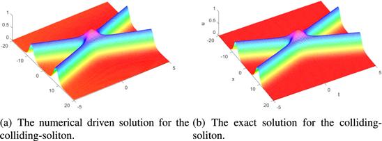
Figure 6. Spatiotemporal evolution of the numerical driven solution and the exact solution for the colliding-soliton. |
From figure 6, we learn the spatiotemporal evolution process of separation-fusion-separation of the colliding-soliton. During the collision, the amplitude remains unchanged, which is consistent with the known fact. The ‘phase shift' phenomenon also occurs in the numerical driven solution.
In order to verify the universality of our neural network architecture for the colliding-soliton, we calculate different colliding-soliton solutions for the Boussinesq equation by the deep learning method. The specific calculation results are shown in table 2. The result shows that the deep learning method is effective in solving the colliding-soliton solution for the Boussinesq equation.
Table 2. The results of different colliding-soliton solutions for the Boussinesq equation calculated by the deep learning method. |
| ${k}_{1}$ | 0.8 | 0.9 | 1.0 | 1.1 | 1.2 |
|---|---|---|---|---|---|
| ${k}_{2}$ | 0.8 | 0.9 | 1.0 | 1.1 | 1.2 |
| ${L}^{2}$ error | $8.55\times {10}^{-2}$ | $8.10\times {10}^{-2}$ | $1.16\times {10}^{-1}$ | $7.63\times {10}^{-2}$ | $7.64\times {10}^{-2}$ |
| Time (s) | 358 | 551 | 642 | 430 | 1065 |
| Iterations | 320 | 635 | 801 | 578 | 755 |
3.2.2. The chasing-soliton for the Boussinesq equation
We could set ${k}_{1}$ = 1.5, ${k}_{2}$ = 0.9, ${\delta }_{1}$ = ${\delta }_{2}$ = 0, ${\omega }_{1}\,$and ${\omega }_{2}$ are positive. In this condition, the two-soliton has same direction and different magnitude, so the soliton chasing phenomenon occurs. We generate the data of 201 snapshots directly on the regular space-time grid with ${\rm{\Delta }}t$ = 0.05 s. A small training data subset is generated by randomly latin hypercube sampling method [34], and the number of collection points is ${N}_{u}$ = 100, ${N}_{f}$ = 25 000. The top panel of figure 7 shows the comparison of the predicted spatiotemporal solution and the exact solution. The middle panel of figure 6 shows the absolute error between the predicted solution and the exact solution. The bottom panel of figure 7 shows the detailed comparison of the exact solution and the learned spatiotemporal solution at different time $t$ = −4.5, $t$ = 0, $t$ = 2.5 respectively. The model achieves a relative ${L}^{2}$ error of size $6.73\times {10}^{-2}$ in a runtime of 892 s.
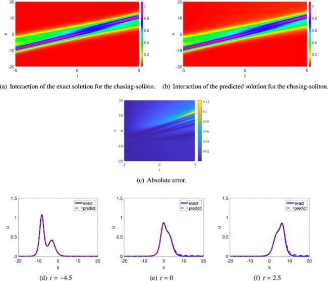
Figure 7. (a), (b) The comparison of the exact solution and the predicted solution for the Boussnesq equation. (c) The absolute error between the exact solution and the predicted solution. (d)–(f) The detailed comparison of the exact solution and the predicted solution at the specific time. |
Figure 8 shows the spatiotemporal evolution process of separation-fusion-separation. Amplitude becomes low during the fusion process and shape remains unchanged before and after the interaction, which is consistent with the known fact. We also observe the ‘phase shift' phenomenon in the chasing-soliton numerical driven solution.
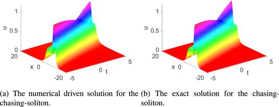
Figure 8. Spatiotemporal evolution of the numerical driven solution and the exact solution for the chasing-soliton. |
In exploring the effectiveness of activation functions, we find tanh function is more effective than the trigonometric function. Taking the one-soliton solution as an example, the calculation results are shown in table 3. The results show that both tanh function and the trigonometric function is useful in the Boussinesq equation, and tanh cost less computational source. Compared with the one-soliton solution, the two-soliton solution for the Boussinesq equation cost more computational source.
Table 3. The results of different activations function of the one-soliton solution for the Boussinesq equation calculated by the deep learning method. |
| Activation function | tanh | cos | sin | Sigmoid | Relu |
|---|---|---|---|---|---|
| ${L}^{2}$ error | $1.97\times {10}^{-2}$ | $1.86\times {10}^{-1}$ | $1.27\times {10}^{-1}$ | $9.22\times {10}^{-1}$ | $8.37\times {10}^{-1}$ |
| Time (s) | 160 | 1670 | 1531 | 105 | 16 |
| Iterations | 195 | 4722 | 3080 | 0 | 4 |
Table 4. The results of different one-soliton solutions for the fifth-order KdV equation calculated by the deep learning method. |
| ${k}_{1}$ | 0.9 | 0.95 | 1.0 | 1.05 | 1.1 |
|---|---|---|---|---|---|
| ${L}^{2}$ error | $1.47\times {10}^{-2}$ | $2.57\times {10}^{-2}$ | $1.36\times {10}^{-2}$ | $4.64\times {10}^{-2}$ | $2.36\times {10}^{-2}$ |
| Time(s) | 687 | 680 | 537 | 600 | 1166 |
| Iterations | 300 | 803 | 803 | 883 | 1604 |
Table 5. The results of different activation functions of the two-soliton solution for the fifth-order KdV equation calculated by the deep learning method. |
| Activation function | tanh | cos | sin | Sigmoid | Relu |
|---|---|---|---|---|---|
| ${L}^{2}$ error | $1.46\times {10}^{-1}$ | $7.22\times {10}^{-2}$ | $1.27\times {10}^{-1}$ | $8.18\times {10}^{-1}$ | $6.13\times {10}^{-1}$ |
| Time (s) | 623 | 1740 | 1531 | 237 | 48 |
| Iterations | 1390 | 3600 | 3080 | 0 | 5 |
4. The numerical driven solution for the fifth-order KdV equation
Consider the initial value problem of the fifth-order KdV equation
$\begin{eqnarray}\left\{\begin{array}{l}{u}_{t}+{(\alpha {u}_{xxxx}+\beta u{u}_{xx}+\gamma {u}^{3})}_{x}=0,\\ u(x,{t}_{0})={u}_{0}(x),\end{array}\right.\end{eqnarray}$
where $\alpha ,$ $\beta ,$ $\gamma $ are arbitrary constant, ${u}_{0}(x)$ is a given real valued smooth function, the subscripts $t$ and $x$ represent partial derivative with respect to time and space respectively.We choose cos as the activation function, and explore the effectiveness of the trigonometric function as the activation function of the fifth-order KdV equation. A deep learning method is used to find the one-soliton and the two-soliton solution of the equation, and reproduce the dynamic behavior between the solitons.
4.1. The one-soliton solution
Using the Hirota bilinear method, the one-soliton analytical solution for the fifth-order KdV equation (9 ) can be obtained [35]
$\begin{eqnarray}\begin{array}{l}u(x,t)=\displaystyle \frac{15\alpha {k}_{1}^{2}}{2\beta }{{\rm{sech}} }^{2}\left(\displaystyle \frac{{{\rm{k}}}_{1}x-\alpha {{\rm{k}}}_{1}^{5}t+{\xi }_{0}}{2}\right).\end{array}\end{eqnarray}$
We set $\alpha $ = 1, $\beta $ = 15, $\gamma $ = 15, ${k}_{1}$ = 1, ${\xi }_{0}=3,$ the equation is also called the C-D-J-K equation. The numerical computation area is truncated in $[-10,10]\times [0,2\pi ]$ for $x$ and $t.$ Correspondingly $\begin{eqnarray}\begin{array}{l}{u}_{0}(x)=\displaystyle \frac{1}{2}{{\rm{sech}} }^{2}\left(\displaystyle \frac{x+3}{2}\right).\end{array}\end{eqnarray}$
In order to obtain the high-precision data set, we generate the data of 201 snapshots directly on the regular space-time grid with ${\rm{\Delta }}t$ = 0.05 s. A small training data subset is generated by randomly latin hypercube sampling method [34], the number of collection points is ${N}_{u}$ = 100, ${N}_{f}$ = 20 000. The top panel of figure 9 shows the comparison of the predicted spatiotemporal solution and the exact solution. The middle panel of figure 9 shows the absolute error between the predicted solution and the exact solution. The bottom panel of figure 9 shows the detailed comparison of the exact solution and the predicted spatiotemporal solution at different time t = 1.57, t = 3.14, 4.71 respectively. Figure 10 shows specific spatiotemporal evolution of the one-soliton solution for the fifth-order KdV equation. The model achieves a relative ${L}^{2}$ error of size $1.36\times {10}^{-2}$ in a runtime of 537 s. The model is iterated 803 times to complete the operation. Figure 11 shows the relationship between the number of function evaluations and ${\rm{L}}{\rm{O}}{\rm{S}}{\rm{S}}$ during calculation.

Figure 9. (a), (b) The comparison of the one-soliton exact solution and the predicted solution for the fifth-order KdV equation. (c) The absolute error between the exact solution and the predicted solution. (d)–(f) The detailed comparison of the exact solution and the predicted solution at the specific time. |
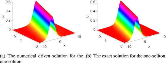
Figure 10. Spatiotemporal evolution of the one-soliton numerical driven solution and the exact solution for the fifth-order KdV equation. |
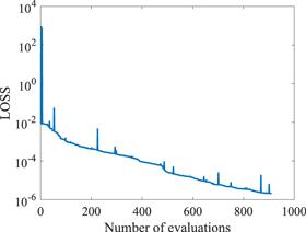
Figure 11. The relationship between the number of function evaluations and ${\rm{L}}{\rm{O}}{\rm{S}}{\rm{S}}.$ |
To verify the universality of the neural network architecture for the one-soliton numerical driven solution for the fifth-order KdV equation, we calculate different one-soliton solutions for the fifth-order KdV equation. The results are shown in table 4. The results show that the neural network architecture is effective in solving the one-soliton solution for the fifth-order KdV equation.
4.2. The two-soliton solution for the fifth-order KdV equation
The numerical computation area is truncated in $[-20,20]\times [-5,5]$ for $x$ and $t.$ By using the Hirota bilinear method, the two-soliton analytical solution for the fifth-order KdV equation can be obtained [35]
$\begin{eqnarray}\begin{array}{l}u(x,t)=2\displaystyle \frac{{k}_{1}^{2}{{\rm{e}}}^{{k}_{1}x+{\omega }_{1}t+{\delta }_{1}}+{k}_{2}^{2}{{\rm{e}}}^{{k}_{2}x+{\omega }_{2}t+{\delta }_{2}}+{({k}_{1}+{k}_{2})}^{2}{{\rm{e}}}^{({k}_{1}+{k}_{2})x+({\omega }_{1}+{\omega }_{2})t+{\delta }_{1}+{\delta }_{2}+{\delta }_{0}}}{1+{{\rm{e}}}^{{k}_{1}x+{\omega }_{1}t+{\delta }_{1}}+{{\rm{e}}}^{{k}_{2}x+{\omega }_{2}t+{\delta }_{2}}+{{\rm{e}}}^{({k}_{1}+{k}_{2})x+({\omega }_{1}+{\omega }_{2})t+{\delta }_{1}+{\delta }_{2}+{\delta }_{0}}}\\ \,-2\displaystyle \frac{{({k}_{1}{{\rm{e}}}^{{k}_{1}x+{\omega }_{1}t+{\delta }_{1}}+{k}_{2}{{\rm{e}}}^{{k}_{2}x+{\omega }_{2}t+{\delta }_{2}}+({k}_{1}+{k}_{2}){{\rm{e}}}^{({k}_{1}+{k}_{2})x+({\omega }_{1}+{\omega }_{2})t+{\delta }_{1}+{\delta }_{2}+{\delta }_{0}})}^{2}}{{(1+{{\rm{e}}}^{{k}_{1}x+{\omega }_{1}t+{\delta }_{1}}+{{\rm{e}}}^{{k}_{2}x+{\omega }_{2}t+{\delta }_{2}}+{{\rm{e}}}^{({k}_{1}+{k}_{2})x+({\omega }_{1}+{\omega }_{2})t+{\delta }_{1}+{\delta }_{2}+{\delta }_{0}})}^{2}},\\ {\omega }_{1}=-{k}_{1}^{5},{\omega }_{2}=-{k}_{2}^{5},{{\rm{e}}}^{{\delta }_{0}}=\displaystyle \frac{{({k}_{1}-{k}_{2})}^{2}+({k}_{1}^{2}-{k}_{1}{k}_{2}+{k}_{2}^{2})}{{({k}_{1}+{k}_{2})}^{2}+({k}_{1}^{2}+{k}_{1}{k}_{2}+{k}_{2}^{2})}.\end{array}\end{eqnarray}$
We could set ${k}_{1}$ = 1, ${k}_{2}$ = 0.8, ${\xi }_{1}={\xi }_{2}=0.$ In order to obtain the high-precision data set, we generate the data of 201 snapshots directly on the regular space-time grid with ${\rm{\Delta }}t$ = 0.05 s. A small training data subset is generated by randomly latin hypercube sampling [34], the number of collection points is ${N}_{u}$ = 100, ${N}_{f}$ = 20 000. The top panel of figure 12 shows the comparison of the predicted spatiotemporal solution and the exact solution. The middle panel of figure 12 shows the absolute error between the predicted solution and the exact solution. The bottom panel of figure 12 shows the detailed comparison of the exact solution and the predicted spatiotemporal solution at different time $t$ = −4.5, $t$ = 0, $t$ = 2.5, respectively. Specific spatiotemporal evolution of the two-soliton is given in figure 13. The model achieves a relative ${L}^{2}$ error of size $7.22\times {10}^{-2}$ in a runtime of 1774s. The model is iterated 3606 times to complete the operation.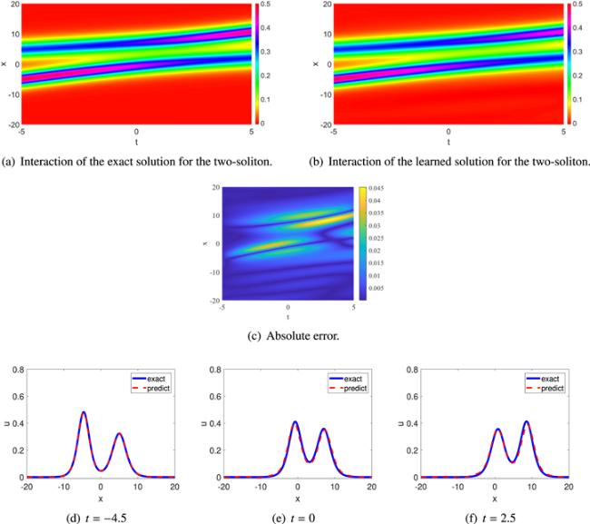
Figure 12. (a), (b) The comparison of the two-soliton exact solution and the predicted solution for the fifth-order KdV equation. (c) The absolute error between the exact solution and the predicted solution. (d)–(f) The detailed comparison of the exact solution and the predicted spatiotemporal solution at the specific time. |

Figure 13. Spatiotemporal evolution of the two-soliton numerical driven solution and the exact solution for the fifth-order KdV equation. |
On the selection of activation functions, a lot of other activation functions have been tested, and the results are given in table 5. The result shows that the trigonometric function is more effective in solving the fifth-order KdV equation.
In addition, the amplitude is changed slightly to verify the rationality of the neural network structure to solve the fifth-order KdV equation. The specific calculation results are shown in the table 6. The results show that the deep learning method is effective in solving the two-soliton solution of the fifth-order KdV equation.
Table 6. The results of different two-soliton solutions for the fifth-order KdV equation calculated by the deep learning method. |
| ${k}_{1}$ | 1.0 | 0.99 | 1.01 | 1.0 | 1.0 |
|---|---|---|---|---|---|
| ${k}_{2}$ | 0.8 | 0.8 | 0.8 | 0.79 | 0.81 |
| ${L}^{2}$ error | $7.22\times {10}^{-2}$ | $8.27\times {10}^{-2}$ | $1.05\times {10}^{-1}$ | $9.05\times {10}^{-2}$ | $1.0\times {10}^{-1}$ |
| Time (s) | 1774 | 913 | 1011 | 1000 | 657 |
| Iterations | 3606 | 1654 | 1738 | 2224 | 1240 |
5. Summary and discussion
We find the suitable architecture of the PINNs for solving high-order nonlinear soliton equations. Specifically, there are four hidden layers, the number of corresponding neurons are 256, 128, 64, 32 and 40, 40, 40, 40. And we study numerical driven solutions of the fourth-order Boussinesq equation and the fifth-order KdV equation, and control ${L}^{2}$ error to ${10}^{-2}$ magnitude, which show that the deep learning method is effective. We extend the deep learning method to the solution of the fourth-order and the fifth-order equation, but the ability of the deep learning method to deal with higher-order equations still needs to be explored.
The conclusions are summarized as follows. Firstly, the deep learning method is suitable to solve the soliton solution for the fourth-order Boussinesq equation and the fifth-order KdV equation. The deep learning method can recover the dynamic behavior of solitons in high-order nonlinear soliton equations. From the numerical driven solution, we can observe the ‘phase shift' phenomenon, and the shape of soliton remains unchanged after the interaction, which is consistent with the known fact. Secondly, the trigonometric function is effective in high-order nonlinear problems. Compared with low-order problems, high-order problems have higher sensitivity in the selection of architecture of the neural network.