


1. Introduction
Quantum entanglement, a magical concept in quantum mechanics, gives rise to many quantum information processes such as quantum teleportation [1], quantum key distribution [2] and quantum computation [3]. Quantum teleportation (QT) is first proposed by Bennett et al [1] in 1993, in which an unknown quantum state is transmitted from a sender Alice to a spatial distant receiver Bob via a previously shared entangled state, assisted with classical communication. Later, Lo [4], Pati [5], and Bennett et al [6] proposed another scheme to transmit a known state, called as remote state preparation (RSP). Compared with QT, the sender has complete knowledge of the transmitted state in RSP, thus there may be a trade-off between the required entanglement and classical communication cost. However, the problem of information leakage may be caused by the dishonest single sender. From this point of view, multiparty RSP schemes such as joint RSP (JRSP) [7–9] and controlled RSP (CRSP) [10–12] were presented to ensure the security of the quantum state transmission process collectively. In JRSP, the information of the prepared state is distributed to more than one senders, they have to cooperate with each other to transmit the initial state to be teleported. At least one controller is involved in CRSP, where the sender and the receiver cannot complete the task without the controllers' permission. In contrast to unidirectional communication, the two-way information exchange between distributed users is more meaningful in realistic quantum communication protocols. In 2014, Cao et al [13] applied bidirectional concept to RSP and devised a scheme named controlled bidirectional RSP (CBRSP) in which the two distant parties are not only senders but also receivers, they can exchange their known state simultaneously under the control of a third party. After that, other CBRSP schemes with multi-participants [14–17] and different quantum channels [18, 19] are investigated successively. As a number of theoretical RSP schemes have sprung up to meet various need, some RSP protocols have been demonstrated experimentally [20–23].
Due to the unavoidably interaction between the system and its surrounding environments, the quantum system gradually loses its coherence, which is a major obstacle for quantum communication. How does the noisy environment affect the RSP process? How to suppress the influence of noises? They are two practical problems that we care about. We notice that there are lots of works analyzing different kinds of RSP process in various noisy environments [24–27]. Generally, due to the memory effects of the non-Markovian environments, the average fidelity exhibits an oscillatory behavior, which is different from the one in Markovian environment with damping exponentially. As far as we know, there are a few researches on bidirectional RSP processes suffering from non-Markovian noise, the noisy environments considered previously are usually Markovian [14, 28–30]. On the other hand, different from traditional von Neumann projective measurement, weak measurement reversal (WMR) is a partially collapsing measurement operation [31–36]. WMR was proven to be helpful for suppressing the decoherence of the entangled states within environment and was utilized for fidelity enhancement in quantum information transmission processes subjected to amplitude damping noise [37–40], which is a type of Markovian noise. In this paper, we examine the protocol for deterministic controlled bidirectional remote preparation of a single qubit state in dissipative environments. After constructing the quantum circuit of the protocol, we derive the corresponding average fidelity analytically. Furthermore, we adopt the methods of WMR and detuning modulation to enhance the average fidelity. Our results show that the amplitude of average fidelity can always be enhanced by the introduction of appropriate WMR and detuning modulation. Compared with the case of Markovian environment, the improvement of the average fidelity in non-Markovian environment is more significant.
The rest of this paper is organized as follows. In section 2 , we describe the bidirectional controlled remote preparation of a single-qubit state and design the corresponding quantum circuit. In section 3 , we calculate the average fidelity of the CBRSP process in dissipative environments. In section 4 , WMR and detuning modulation are applied to further improve the average fidelity. Finally, a summary is given in section 5 .
2. Controlled bidirectional remote preparation of an arbitrary single-qubit state
In this section, we describe the CBRSP protocol in which Alice and Bob are not only the senders but also the receivers. They wish to prepare a known single qubit for each other under the help of the controller Charlie. Assume that Alice wants to help Bob prepare a single qubit $\left|{\varphi }_{1}\right\rangle $ known by her, and meanwhile Bob wants to prepare a single qubit $\left|{\varphi }_{2}\right\rangle $ known by him for Alice. The single qubit they want to prepare at each other's side takes the form
$\begin{eqnarray}\left|{\varphi }_{j}\right\rangle =\cos \displaystyle \frac{{\theta }_{j}}{2}\left|0\right\rangle +\sin \displaystyle \frac{{\theta }_{j}}{2}{{\rm{e}}}^{{\rm{i}}{\phi }_{j}}\left|1\right\rangle ,(j=1,2),\end{eqnarray}$
where θj and φj are the polar and azimuthal angles of the qubit with θj ∈ [0, π] and φj ∈ [0, 2π]. To achieve the CBRSP task, Alice and Bob are assumed to share two same EPR states ${\left|\psi \right\rangle }_{12}=\tfrac{1}{\sqrt{2}}({\left|01\right\rangle }_{12}+{\left|10\right\rangle }_{12})$ and ${\left|\psi \right\rangle }_{34}=\tfrac{1}{\sqrt{2}}({\left|01\right\rangle }_{34}\,+{\left|10\right\rangle }_{34})$, where qubits 1 and 4 belong to Alice and qubits 2 and 3 belong to Bob, while the controller Charlie at Alice's side holds the qubit 5 with the initial state $\left|0\right\rangle $. Now Charlie performs a Hadamard operation on his qubit 5. In this way, the five-qubit state consisting of the qubits 1, 2, 3, 4, and 5 becomes $\begin{eqnarray}\begin{array}{rcl}{\left|{\rm{\Psi }}\right\rangle }_{12345} & = & \displaystyle \frac{1}{2\sqrt{2}}[{\left(\left|01\right\rangle +\left|10\right\rangle \right)}_{12}{\left(\left|01\right\rangle +\left|10\right\rangle \right)}_{34}{\left|0\right\rangle }_{5}\\ & & +{\left(\left|01\right\rangle +\left|10\right\rangle \right)}_{12}{\left(\left|01\right\rangle +\left|10\right\rangle \right)}_{34}{\left|1\right\rangle }_{5}].\end{array}\end{eqnarray}$
Afterwards, Charlie makes ${\left({\sigma }_{z}\right)}_{5\to 1}$ and ${({\sigma }_{z})}_{5\to 4}$ transformation on his qubit and Alice's qubit, respectively, where ${\left({\sigma }_{z}\right)}_{5\to k}$ denotes a two-qubit controlled-Σz operation with 5 as the controlled qubit and k (k = 1 or 4) as the target qubit. Moreover, Alice performs Σx operation on qubit 4 while Bob performs Σx operation on qubit 2 . Here ${\sigma }_{x}=\left(\begin{array}{cc}0 & 1\\ 1 & 0\end{array}\right)\ $ and ${\sigma }_{z}=\left(\begin{array}{cc}1 & 0\\ 0 & -1\end{array}\right)$ are two Pauli matrices. In this situation, the five-qubit state ${\left|{\rm{\Psi }}\right\rangle }_{12345}$ can be reexpressed as
$\begin{eqnarray}\begin{array}{rcl}{\left|{{\rm{\Psi }}}^{{\prime} }\right\rangle }_{12345} & = & \displaystyle \frac{1}{2\sqrt{2}}[{\left(\left|00\right\rangle +\left|11\right\rangle \right)}_{12}{\left(\left|00\right\rangle +\left|11\right\rangle \right)}_{34}{\left|0\right\rangle }_{5}\\ & & -{\left(\left|00\right\rangle -\left|11\right\rangle \right)}_{12}{\left(\left|00\right\rangle -\left|11\right\rangle \right)}_{34}{\left|1\right\rangle }_{5}].\end{array}\end{eqnarray}$
Now Alice (Bob) introduces an auxiliary qubit ${1}^{{\prime} }$ $({3}^{{\prime} })$ with the initial state $\left|0\right\rangle $, and then performs a controlled-NOT operation on her (his) own two qubits 1 and ${1}^{{\prime} }$ (3 and ${3}^{{\prime} })$ with particle 1 (3) as the controlled qubit and particle ${1}^{{\prime} }$ $({3}^{{\prime} })$ as the target one accordingly. At this stage, the total state of the quantum channel shared among Alice, Bob and Charlie consisting of the seven qubits 1, ${1}^{{\prime} }$, 2, 3, ${3}^{{\prime} }$, 4, 5 is given by
$\begin{eqnarray}\begin{array}{l}{\left|{\rm{\Psi }}\right\rangle }_{{11}^{{\prime} }{233}^{{\prime} }45}=\displaystyle \frac{1}{2\sqrt{2}}[{\left(\left|000\right\rangle +\left|111\right\rangle \right)}_{{11}^{{\prime} }2}{\left(\left|000\right\rangle +\left|111\right\rangle \right)}_{{33}^{{\prime} }4}{\left|0\right\rangle }_{5}\\ \ \ -\ {\left(\left|000\right\rangle -\left|111\right\rangle \right)}_{{11}^{{\prime} }2}{\left(\left|000\right\rangle -\left|111\right\rangle \right)}_{{33}^{{\prime} }4}{\left|1\right\rangle }_{5}].\end{array}\end{eqnarray}$
After the quantum channel is set up, Alice and Bob need to achieve the bidirectional RSP protocol. As for Alice, who has complete knowledge of the initial state $\left|{\varphi }_{1}\right\rangle $, she wants to help Bob reconstruct the state remotely with the assistance of Charlie. To this end, she carries out a single-qubit projective measurement on her particle 1 in the basis $\left\{\left|{\mu }_{0}\right\rangle ,\left|{\mu }_{1}\right\rangle \right\}$, which is related to the amplitude information described by the parameter θ1 with the following relation $\begin{eqnarray}\left(\begin{array}{c}{\left|{\mu }_{0}\right\rangle }_{1}\\ {\left|{\mu }_{1}\right\rangle }_{1}\end{array}\right)=\left(\begin{array}{c}\cos \tfrac{{\theta }_{1}}{2}\\ \sin \tfrac{{\theta }_{1}}{2}\end{array}\begin{array}{c}\,\sin \tfrac{{\theta }_{1}}{2}\\ \,-\cos \tfrac{{\theta }_{1}}{2}\end{array}\right)\left(\begin{array}{c}{\left|0\right\rangle }_{1}\\ {\left|1\right\rangle }_{1}\end{array}\right).\end{eqnarray}$
Therefore the total state ${\left|{\rm{\Psi }}\right\rangle }_{{11}^{{\prime} }{233}^{{\prime} }45}$ can be expanded as $\begin{eqnarray}\begin{array}{rcl}{\left|{\rm{\Psi }}\right\rangle }_{{11}^{{\prime} }{233}^{{\prime} }45} & = & \displaystyle \frac{1}{2\sqrt{2}}[{\left|{\mu }_{0}\right\rangle }_{1}{\left(\cos \displaystyle \frac{{\theta }_{1}}{2}\left|00\right\rangle +\sin \displaystyle \frac{{\theta }_{1}}{2}\left|11\right\rangle \right)}_{{1}^{{\prime} }2}{\left(\left|000\right\rangle +\left|111\right\rangle \right)}_{{33}^{{\prime} }4}{\left|0\right\rangle }_{5}\\ & & -{\left|{\mu }_{0}\right\rangle }_{1}{\left(\cos \displaystyle \frac{{\theta }_{1}}{2}\left|00\right\rangle -\sin \displaystyle \frac{{\theta }_{1}}{2}\left|11\right\rangle \right)}_{{1}^{{\prime} }2}{\left(\left|000\right\rangle -\left|111\right\rangle \right)}_{{33}^{{\prime} }4}{\left|1\right\rangle }_{5}\\ & & +{\left|{\mu }_{1}\right\rangle }_{1}{\left(\sin \displaystyle \frac{{\theta }_{1}}{2}\left|00\right\rangle -\cos \displaystyle \frac{{\theta }_{1}}{2}\left|11\right\rangle \right)}_{{1}^{{\prime} }2}{\left(\left|000\right\rangle +\left|111\right\rangle \right)}_{{33}^{{\prime} }4}{\left|0\right\rangle }_{5}\\ & & -{\left|{\mu }_{1}\right\rangle }_{1}{\left(\sin \displaystyle \frac{{\theta }_{1}}{2}\left|00\right\rangle +\cos \displaystyle \frac{{\theta }_{1}}{2}\left|11\right\rangle \right)}_{{1}^{{\prime} }2}{\left(\left|000\right\rangle -\left|111\right\rangle \right)}_{{33}^{{\prime} }4}{\left|1\right\rangle }_{5}].\end{array}\end{eqnarray}$
Now Alice informs Bob of her measurement result via classical communication. To help Bob restore the initial state $\left|{\varphi }_{1}\right\rangle $, Alice and Bob need to make some suitable unitary operations on their qubits. If Alice's measurement outcome of qubit 1 is ${\left|{\mu }_{1}\right\rangle }_{1}$, then she applies Σx operation on her qubit ${1}^{{\prime} }$ and Bob applies −iΣy operation on his qubit 2. Otherwise, if Alice's measurement outcome of qubit 1 is ${\left|{\mu }_{0}\right\rangle }_{1}$, she and Bob perform identity operations I on the qubits ${1}^{{\prime} }$ and 2 respectively. In this case, the total sate ${\left|{\rm{\Psi }}\right\rangle }_{{11}^{{\prime} }{233}^{{\prime} }45}$ can be reexpressed as6 ) can then be rewritten as
$\begin{eqnarray}\begin{array}{rcl}{\left|{\rm{\Psi }}\right\rangle }_{{11}^{{\prime} }{233}^{{\prime} }45} & = & \displaystyle \frac{1}{2\sqrt{2}}\{{\left|{\mu }_{0}\right\rangle }_{1}{\left(\cos \displaystyle \frac{{\theta }_{1}}{2}\left|00\right\rangle +\sin \displaystyle \frac{{\theta }_{1}}{2}\left|11\right\rangle \right)}_{{1}^{{\prime} }2}{\left(\left|000\right\rangle +\left|111\right\rangle \right)}_{{33}^{{\prime} }4}{\left|0\right\rangle }_{5}\\ & & -{\left|{\mu }_{0}\right\rangle }_{1}{\left(\cos \displaystyle \frac{{\theta }_{1}}{2}\left|00\right\rangle -\sin \displaystyle \frac{{\theta }_{1}}{2}\left|11\right\rangle \right)}_{{1}^{{\prime} }2}{\left(\left|000\right\rangle -\left|111\right\rangle \right)}_{{33}^{{\prime} }4}{\left|1\right\rangle }_{5}\\ & & +{\left|{\mu }_{1}\right\rangle }_{1}[{\left({\sigma }_{x}\right)}_{{1}^{{\prime} }}\otimes {\left({\rm{i}}{\sigma }_{y}\right)}_{2}]{\left(\sin \displaystyle \frac{{\theta }_{1}}{2}\left|11\right\rangle +\cos \displaystyle \frac{{\theta }_{1}}{2}\left|00\right\rangle \right)}_{{1}^{{\prime} }2}{\left(\left|000\right\rangle +\left|111\right\rangle \right)}_{{33}^{{\prime} }4}{\left|0\right\rangle }_{5}\\ & & -{\left|{\mu }_{1}\right\rangle }_{1}[{\left({\sigma }_{x}\right)}_{{1}^{{\prime} }}\otimes {\left({\rm{i}}{\sigma }_{y}\right)}_{2}]{\left(\sin \displaystyle \frac{{\theta }_{1}}{2}\left|11\right\rangle -\cos \displaystyle \frac{{\theta }_{1}}{2}\left|00\right\rangle \right)}_{{1}^{{\prime} }2}{\left(\left|000\right\rangle -\left|111\right\rangle \right)}_{{33}^{{\prime} }4}{\left|1\right\rangle }_{5}\}.\end{array}\end{eqnarray}$
Here, $I=\left(\begin{array}{cc}1 & 0\\ 0 & 1\end{array}\right)$ is an identity matrix, and ${\sigma }_{y}=\left(\begin{array}{cc}0 & -{\rm{i}}\\ {\rm{i}} & 0\end{array}\right)$ is a Pauli matrix. Subsequently, Alice proceeds to measure her particle ${1}^{{\prime} }$ on the basis of the phase information described by the parameter φ1 as follows $\begin{eqnarray}\left(\begin{array}{c}{\left|{v}_{0}\right\rangle }_{{1}^{{\prime} }}\\ {\left|{v}_{1}\right\rangle }_{{1}^{{\prime} }}\end{array}\right)=\displaystyle \frac{1}{\sqrt{2}}\left(\begin{array}{c}1\\ 1\end{array}\begin{array}{c}\,{{\rm{e}}}^{-{\rm{i}}{\phi }_{1}}\\ \,-{{\rm{e}}}^{-{\rm{i}}{\phi }_{1}}\end{array}\right)\left(\begin{array}{c}{\left|0\right\rangle }_{{1}^{{\prime} }}\\ {\left|1\right\rangle }_{{1}^{{\prime} }}\end{array}\right).\end{eqnarray}$
The total state in equation ( $\begin{eqnarray}\begin{array}{rcl}{\left|{\rm{\Psi }}\right\rangle }_{{11}^{{\prime} }{233}^{{\prime} }45} & = & \frac{1}{4}[({\left|{\mu }_{0}\right\rangle }_{1}{\left|{v}_{0}\right\rangle }_{{1}^{{\prime} }}+{\left|{\mu }_{1}\right\rangle }_{1}[{\left({\sigma }_{x}\right)}_{{1}^{{\prime} }}\otimes {\left({\rm{i}}{\sigma }_{y}\right)}_{2}]{\left|{v}_{0}\right\rangle }_{{1}^{{\prime} }}){\left(\cos \frac{{\theta }_{1}}{2}\left|0\right\rangle +\sin \frac{{\theta }_{1}}{2}{{\rm{e}}}^{{\rm{i}}{\phi }_{1}}\left|1\right\rangle \right)}_{2}{\left(\left|000\right\rangle +\left|111\right\rangle \right)}_{{33}^{{\prime} }4}{\left|0\right\rangle }_{5}\\ & & +({\left|{\mu }_{0}\right\rangle }_{1}{\left|{v}_{1}\right\rangle }_{{1}^{{\prime} }}+{\left|{\mu }_{1}\right\rangle }_{1}[{\left({\sigma }_{x}\right)}_{{1}^{{\prime} }}\otimes {\left({\rm{i}}{\sigma }_{y}\right)}_{2}]{\left|{v}_{1}\right\rangle }_{{1}^{{\prime} }}){\left(\cos \frac{{\theta }_{1}}{2}\left|0\right\rangle -\sin \frac{{\theta }_{1}}{2}{{\rm{e}}}^{{\rm{i}}{\phi }_{1}}\left|1\right\rangle \right)}_{2}{\left(\left|000\right\rangle +\left|111\right\rangle \right)}_{{33}^{{\prime} }4}{\left|0\right\rangle }_{5}\\ & & -({\left|{\mu }_{0}\right\rangle }_{1}{\left|{v}_{0}\right\rangle }_{{1}^{{\prime} }}-{\left|{\mu }_{1}\right\rangle }_{1}[{\left({\sigma }_{x}\right)}_{{1}^{{\prime} }}\otimes {\left({\rm{i}}{\sigma }_{y}\right)}_{2}]{\left|{v}_{0}\right\rangle }_{{1}^{{\prime} }}){\left(\cos \frac{{\theta }_{1}}{2}\left|0\right\rangle -\sin \frac{{\theta }_{1}}{2}{{\rm{e}}}^{{\rm{i}}{\phi }_{1}}\left|1\right\rangle \right)}_{2}{\left(\left|000\right\rangle -\left|111\right\rangle \right)}_{{33}^{{\prime} }4}{\left|1\right\rangle }_{5}\\ & & -({\left|{\mu }_{0}\right\rangle }_{1}{\left|{v}_{1}\right\rangle }_{{1}^{{\prime} }}-{\left|{\mu }_{1}\right\rangle }_{1}[{\left({\sigma }_{x}\right)}_{{1}^{{\prime} }}\otimes {\left({\rm{i}}{\sigma }_{y}\right)}_{2}]{\left|{v}_{1}\right\rangle }_{{1}^{{\prime} }}){\left(\cos \frac{{\theta }_{1}}{2}\left|0\right\rangle +\sin \frac{{\theta }_{1}}{2}{{\rm{e}}}^{{\rm{i}}{\phi }_{1}}\left|1\right\rangle \right)}_{2}{\left(\left|000\right\rangle -\left|111\right\rangle \right)}_{{33}^{{\prime} }4}{\left|1\right\rangle }_{5}].\end{array}\end{eqnarray}$
At this moment, if the result of Alice's measurement on particle ${1}^{{\prime} }$ is ${\left|{v}_{1}\right\rangle }_{{1}^{{\prime} }}$, Bob carries out Pauli Σz operation on his qubit 2. Otherwise, if Alice's measurement outcome of qubit 1′ is ${\left|{v}_{0}\right\rangle }_{{1}^{{\prime} }}$, Bob does not need to perform any operations on his particle 2 . In this way, the total state ${\left|{\rm{\Psi }}\right\rangle }_{{11}^{{\prime} }{233}^{{\prime} }45}$ is given by $\begin{eqnarray}\begin{array}{rcl}{\left|{\rm{\Psi }}\right\rangle }_{{11}^{{\prime} }{233}^{{\prime} }45} & = & \frac{1}{4}[({\left|{\mu }_{0}\right\rangle }_{1}{\left|{v}_{0}\right\rangle }_{{1}^{{\prime} }}+{\left|{\mu }_{1}\right\rangle }_{1}[{\left({\sigma }_{x}\right)}_{{1}^{{\prime} }}\otimes {\left({\rm{i}}{\sigma }_{y}\right)}_{2}]{\left|{v}_{0}\right\rangle }_{{1}^{{\prime} }}){\left(\cos \frac{{\theta }_{1}}{2}\left|0\right\rangle +\sin \frac{{\theta }_{1}}{2}{{\rm{e}}}^{{\rm{i}}{\phi }_{1}}\left|1\right\rangle \right)}_{2}{\left(\left|000\right\rangle +\left|111\right\rangle \right)}_{{33}^{{\prime} }4}{\left|0\right\rangle }_{5}\\ & & +({\left|{\mu }_{0}\right\rangle }_{1}{\left|{v}_{1}\right\rangle }_{{1}^{{\prime} }}+{\left|{\mu }_{1}\right\rangle }_{1}[{\left({\sigma }_{x}\right)}_{{1}^{{\prime} }}\otimes {\left({\rm{i}}{\sigma }_{y}\right)}_{2}]{\left|{v}_{1}\right\rangle }_{{1}^{{\prime} }}){\left({\sigma }_{z}\right)}_{2}{\left(\cos \frac{{\theta }_{1}}{2}\left|0\right\rangle +\sin \frac{{\theta }_{1}}{2}{{\rm{e}}}^{{\rm{i}}{\phi }_{1}}\left|1\right\rangle \right)}_{2}{\left(\left|000\right\rangle +\left|111\right\rangle \right)}_{{33}^{{\prime} }4}{\left|0\right\rangle }_{5}\\ & & -({\left|{\mu }_{0}\right\rangle }_{1}{\left|{v}_{0}\right\rangle }_{{1}^{{\prime} }}-{\left|{\mu }_{1}\right\rangle }_{1}[{\left({\sigma }_{x}\right)}_{{1}^{{\prime} }}\otimes {\left({\rm{i}}{\sigma }_{y}\right)}_{2}]{\left|{v}_{0}\right\rangle }_{{1}^{{\prime} }}){\left(\cos \frac{{\theta }_{1}}{2}\left|0\right\rangle -\sin \frac{{\theta }_{1}}{2}{{\rm{e}}}^{{\rm{i}}{\phi }_{1}}\left|1\right\rangle \right)}_{2}{\left(\left|000\right\rangle -\left|111\right\rangle \right)}_{{33}^{{\prime} }4}{\left|1\right\rangle }_{5}\\ & & -({\left|{\mu }_{0}\right\rangle }_{1}{\left|{v}_{1}\right\rangle }_{{1}^{{\prime} }}-{\left|{\mu }_{1}\right\rangle }_{1}[{\left({\sigma }_{x}\right)}_{{1}^{{\prime} }}\otimes {\left({\rm{i}}{\sigma }_{y}\right)}_{2}]{\left|{v}_{1}\right\rangle }_{{1}^{{\prime} }}){\left({\sigma }_{z}\right)}_{2}{\left(\cos \frac{{\theta }_{1}}{2}\left|0\right\rangle -\sin \frac{{\theta }_{1}}{2}{{\rm{e}}}^{{\rm{i}}{\phi }_{1}}\left|1\right\rangle \right)}_{2}{\left(\left|000\right\rangle -\left|111\right\rangle \right)}_{{33}^{{\prime} }4}{\left|1\right\rangle }_{5}].\end{array}\end{eqnarray}$
On the other hand, as for Bob, who has complete knowledge of the initial state $\left|{\varphi }_{2}\right\rangle $, he wants to help Alice prepare the state remotely. Since our CBRSP protocol is a symmetric one, Bob just needs to follow Alice's previous operations in a similar manner. In other words, Bob first measures his qubit 3 on the basis $\left\{\left|{\mu }_{0}^{{\prime} }\right\rangle ,\ \left|{\mu }_{1}^{{\prime} }\right\rangle \right\}$, which is related to the amplitude information described by the parameter θ2 with the following relation
$\begin{eqnarray}\left(\begin{array}{c}{\left|{\mu }_{0}^{{\prime} }\right\rangle }_{3}\\ {\left|{\mu }_{1}^{{\prime} }\right\rangle }_{3}\end{array}\right)=\left(\begin{array}{c}\cos \displaystyle \frac{{\theta }_{2}}{2}\\ \sin \displaystyle \frac{{\theta }_{2}}{2}\end{array}\begin{array}{c}\,\sin \displaystyle \frac{{\theta }_{2}}{2}\\ \,-\cos \displaystyle \frac{{\theta }_{2}}{2}\end{array}\right)\left(\begin{array}{c}{\left|0\right\rangle }_{3}\\ {\left|1\right\rangle }_{3}\end{array}\right).\end{eqnarray}$
According to his measurement results via classical communication, Bob and Alice need to perform suitable unitary operations on their respective qubits locally. Specifically, if Bob's measurement result is ${\left|{\mu }_{1}^{{\prime} }\right\rangle }_{3}$, then he makes Σx operation on his qubit ${3}^{{\prime} }$ and Alice makes −iΣy operation on her qubit 4. Otherwise, if Bob's measurement result is ${\left|{\mu }_{0}^{{\prime} }\right\rangle }_{3}$, they do not need to perform any operations on their qubits. Subsequently, Bob performs the phase-dependent measurement on his particle ${3}^{{\prime} }$ with the following basis $\begin{eqnarray}\left(\begin{array}{c}{\left|{v}_{0}^{{\prime} }\right\rangle }_{{3}^{{\prime} }}\\ {\left|{v}_{1}^{{\prime} }\right\rangle }_{{3}^{{\prime} }}\end{array}\right)=\displaystyle \frac{1}{\sqrt{2}}\left(\begin{array}{c}1\\ 1\end{array}\begin{array}{c}\,{{\rm{e}}}^{-{\rm{i}}{\phi }_{2}}\\ \,-{{\rm{e}}}^{-{\rm{i}}{\phi }_{2}}\end{array}\right)\left(\begin{array}{c}{\left|0\right\rangle }_{{1}^{{\prime} }}\\ {\left|1\right\rangle }_{{1}^{{\prime} }}\end{array}\right).\end{eqnarray}$
Only if Bob's measurement result is ${\left|{v}_{1}^{{\prime} }\right\rangle }_{{3}^{{\prime} }}$, Alice needs to carry out Σz operation on her qubit 4. None of unitary transformations is required for Bob's measurement result being ${\left|{v}_{0}^{{\prime} }\right\rangle }_{{3}^{{\prime} }}$. After Bob's two-step measurements depending on amplitude and phase information of the state $\left|{\varphi }_{2}\right\rangle $, the total state ${\left|{\rm{\Psi }}\right\rangle }_{{11}^{{\prime} }{233}^{{\prime} }45}$ is transformed to $\begin{eqnarray}\begin{array}{rcl}{\left|{{\rm{\Psi }}}^{{\prime} }\right\rangle }_{{11}^{{\prime} }{233}^{{\prime} }45} & = & \displaystyle \frac{1}{4\sqrt{2}}[({\left|{\mu }_{0}\right\rangle }_{1}{\left|{v}_{0}\right\rangle }_{{1}^{{\prime} }}{\left|{\mu }_{0}^{{\prime} }\right\rangle }_{3}{\left|{v}_{0}^{{\prime} }\right\rangle }_{{3}^{{\prime} }}+{\left|{\mu }_{0}\right\rangle }_{1}{\left|{v}_{1}\right\rangle }_{{1}^{{\prime} }}{\left|{\mu }_{0}^{{\prime} }\right\rangle }_{3}{\left|{v}_{1}^{{\prime} }\right\rangle }_{{3}^{{\prime} }}+{\left|{\mu }_{1}\right\rangle }_{1}{\left|{v}_{0}\right\rangle }_{{1}^{{\prime} }}{\left|{\mu }_{1}^{{\prime} }\right\rangle }_{3}{\left|{v}_{0}^{{\prime} }\right\rangle }_{{3}^{{\prime} }}\\ & & +{\left|{\mu }_{1}\right\rangle }_{1}{\left|{v}_{1}\right\rangle }_{{1}^{{\prime} }}{\left|{\mu }_{1}^{{\prime} }\right\rangle }_{3}{\left|{v}_{1}^{{\prime} }\right\rangle }_{{3}^{{\prime} }}){\left(\cos \displaystyle \frac{{\theta }_{1}}{2}\left|0\right\rangle +\sin \displaystyle \frac{{\theta }_{1}}{2}{{\rm{e}}}^{{\rm{i}}{\phi }_{1}}\left|1\right\rangle \right)}_{2}{\left(\cos \displaystyle \frac{{\theta }_{2}}{2}\left|0\right\rangle +\sin \displaystyle \frac{{\theta }_{2}}{2}{{\rm{e}}}^{{\rm{i}}{\phi }_{2}}\left|1\right\rangle \right)}_{4}{\left|0\right\rangle }_{5}\\ & & -({\left|{\mu }_{0}\right\rangle }_{1}{\left|{v}_{0}\right\rangle }_{{1}^{{\prime} }}{\left|{\mu }_{0}^{{\prime} }\right\rangle }_{3}{\left|{v}_{0}^{{\prime} }\right\rangle }_{{3}^{{\prime} }}+{\left|{\mu }_{0}\right\rangle }_{1}{\left|{v}_{1}\right\rangle }_{{1}^{{\prime} }}{\left|{\mu }_{0}^{{\prime} }\right\rangle }_{3}{\left|{v}_{1}^{{\prime} }\right\rangle }_{{3}^{{\prime} }}+{\left|{\mu }_{1}\right\rangle }_{1}{\left|{v}_{0}\right\rangle }_{{1}^{{\prime} }}{\left|{\mu }_{1}^{{\prime} }\right\rangle }_{3}{\left|{v}_{0}^{{\prime} }\right\rangle }_{{3}^{{\prime} }}\\ & & +{\left|{\mu }_{1}\right\rangle }_{1}{\left|{v}_{1}\right\rangle }_{{1}^{{\prime} }}{\left|{\mu }_{1}^{{\prime} }\right\rangle }_{3}{\left|{v}_{1}^{{\prime} }\right\rangle }_{{3}^{{\prime} }}){\left(\cos \displaystyle \frac{{\theta }_{1}}{2}\left|0\right\rangle -\sin \displaystyle \frac{{\theta }_{1}}{2}{{\rm{e}}}^{{\rm{i}}{\phi }_{1}}\left|1\right\rangle \right)}_{2}{\left(\cos \displaystyle \frac{{\theta }_{2}}{2}\left|0\right\rangle -\sin \displaystyle \frac{{\theta }_{2}}{2}{{\rm{e}}}^{{\rm{i}}{\phi }_{2}}\left|1\right\rangle \right)}_{4}{\left|1\right\rangle }_{5}].\end{array}\end{eqnarray}$
At this stage, Alice (Bob) informs Bob (Alice) and Charlie of their measurement results through classical communication. Obviously Alice and Bob could not achieve their tasks without Charlie's help. Now Charlie performs the projective measurement on his qubit 5 with measurement basis $\{{\left|0\right\rangle }_{5}$, ${\left|1\right\rangle }_{5}\}$. If Charlie's measurement result is ${\left|0\right\rangle }_{5}$, the collapse state of qubit 4 at Alice's side is $\left|{\varphi }_{2}\right\rangle =\cos \tfrac{{\theta }_{2}}{2}\left|0\right\rangle +\sin \tfrac{{\theta }_{2}}{2}{{\rm{e}}}^{{\rm{i}}{\phi }_{2}}\left|1\right\rangle $, which is the desired state that Bob plans to prepare for Alice. Meanwhile, qubit 2 at Bob's side is collapsed to the desired state $\left|{\varphi }_{1}\right\rangle =\cos \tfrac{{\theta }_{1}}{2}\left|0\right\rangle +\sin \tfrac{{\theta }_{1}}{2}{{\rm{e}}}^{{\rm{i}}{\phi }_{1}}\left|1\right\rangle $ to be remotely prepared for Bob. Otherwise, if Charlie's measurement result is ${\left|1\right\rangle }_{5}$, the collapsed state of qubit 4 at Alice's side is $\left|{\varphi }_{2}\right\rangle =\cos \tfrac{{\theta }_{2}}{2}\left|0\right\rangle -\sin \tfrac{{\theta }_{2}}{2}{{\rm{e}}}^{{\rm{i}}{\phi }_{2}}\left|1\right\rangle $ while the collapse state of qubit 2 at Bob's side is $\left|{\varphi }_{1}\right\rangle =\cos \tfrac{{\theta }_{1}}{2}\left|0\right\rangle -\sin \tfrac{{\theta }_{1}}{2}{{\rm{e}}}^{{\rm{i}}{\phi }_{1}}\left|1\right\rangle ,$ except for an unimportant common phase factor. To help Alice and Bob receive the desired state respectively, Charlie informs Alice and Bob of his measurement result. In this way, if the result of Charlie's measurement is ${\left|1\right\rangle }_{5}$, after Alice and Bob performs Pauli operation Σz on the qubits 4 and 2, respectively, the qubit 4 at Alice's side is in the desired state $\left|{\varphi }_{2}\right\rangle =\cos \tfrac{{\theta }_{2}}{2}\left|0\right\rangle +\sin \tfrac{{\theta }_{2}}{2}{{\rm{e}}}^{{\rm{i}}{\phi }_{2}}\left|1\right\rangle $, while the state of qubit 2 at Bob's side is $\left|{\varphi }_{1}\right\rangle =\cos \tfrac{{\theta }_{1}}{2}\left|0\right\rangle +\sin \tfrac{{\theta }_{1}}{2}{{\rm{e}}}^{{\rm{i}}{\phi }_{1}}\left|1\right\rangle $. As a consequence, bidirectional controlled remote preparation of the arbitrary single qubit can be realized deterministically with unit success probability.
Based on the above procedures, we design the complete quantum circuit of the CBRSP protocol in figure 1, where the dot ‘•' denotes the control qubit, ‘ ⊕ ', ‘Σx', ‘ − iΣy', ‘Σz' denote the target qubits, ‘H' is the Hadamard gate, ‘M1', ‘${M}_{{1}^{{\prime} }}$', ‘M3', ‘${M}_{{3}^{{\prime} }}$', ‘M5' represent the single-qubit projective measurements, and the double line represents the classical information. The single-qubit unitary amplitude operators U1 and U2, and the single-qubit unitary phase operators V1 and V2 take the following respective forms
$\begin{eqnarray}\begin{array}{rcl}{U}_{1} & = & \left(\begin{array}{cc}\cos \tfrac{{\theta }_{1}}{2} & \sin \tfrac{{\theta }_{1}}{2}\\ \sin \tfrac{{\theta }_{1}}{2} & -\cos \tfrac{{\theta }_{1}}{2}\end{array}\right),{U}_{2}=\left(\begin{array}{cc}\cos \tfrac{{\theta }_{2}}{2} & \sin \tfrac{{\theta }_{2}}{2}\\ \sin \tfrac{{\theta }_{2}}{2} & -\cos \tfrac{{\theta }_{2}}{2}\end{array}\right),\\ {V}_{1} & = & \displaystyle \frac{1}{\sqrt{2}}\left(\begin{array}{cc}1 & {{\rm{e}}}^{-{\rm{i}}{\phi }_{1}}\\ 1 & -{{\rm{e}}}^{-{\rm{i}}{\phi }_{1}}\end{array}\right),{V}_{2}=\displaystyle \frac{1}{\sqrt{2}}\left(\begin{array}{cc}1 & {{\rm{e}}}^{-{\rm{i}}{\phi }_{2}}\\ 1 & -{{\rm{e}}}^{-{\rm{i}}{\phi }_{2}}\end{array}\right).\end{array}\end{eqnarray}$
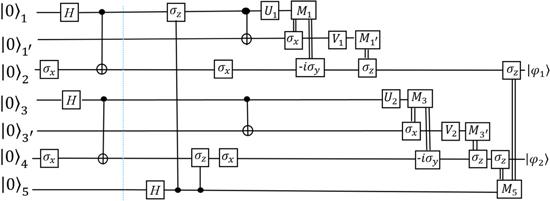
Figure 1. Quantum circuit for deterministic bidirectional controlled remote preparation of a single-qubit state. Here the qubits 1, ${1}^{{\prime} }$ and 4 belong to Alice, the qubits 2, 3 and ${3}^{{\prime} }$ belong to Bob, and the qubit 5 belongs to Charlie at Alice's side. |
3. Non-Markovian effects on the deterministic CBRSP process
It is widely accepted that a quantum system will inevitably interact with its surrounding environment, resulting in the loss of systemic coherence. In what follows, we turn to explore the dynamics of our CBRSP protocol under the influence of dissipative environments. Explicitly, we assume that the initial entangled pairs ${\left|\psi \right\rangle }_{12}$ and ${\left|\psi \right\rangle }_{34}$ shared by Alice and Bob are coupled with their respective vacuum reservoirs at zero temperature independently. The single-qubit reservoir Hamiltonian [41] (in units of ℏ = 1) is given by
$\begin{eqnarray}H={\omega }_{0}{\sigma }_{+}{\sigma }_{-}+\sum _{k}{\omega }_{k}{b}_{k}^{\dagger }{b}_{k}+\sum _{k}({g}_{k}{\sigma }_{+}{b}_{k}+{g}_{k}^{* }{\sigma }_{-}{b}_{k}^{\dagger }),\end{eqnarray}$
where ω0 is the transition frequency of the two-level system, Σ+ (Σ−) is the raising (lowering) operator of the qubit, the index k denotes the field modes of the reservoir with frequencies ωk, ${b}_{k}^{\dagger }$ and bk are the creation and annihilation operators of the reservoir mode k, and gk is the coupling constant between qubit and reservoir with mode k. The dynamics of the single qubit S [42] can be described by the reduced density matrix $\begin{eqnarray}{\rho }^{S}(t)=\left(\begin{array}{cc}{\rho }_{11}^{S}(0){\left|\xi \left(t\right)\right|}^{2} & {\rho }_{10}^{S}(0)\xi \left(t\right)\\ {\rho }_{01}^{S}(0)\ {\xi }^{* }\left(t\right) & {\rho }_{00}^{S}(0)+{\rho }_{11}^{S}(0)[1-{\left|\xi \left(t\right)\right|}^{2}]\end{array}\right),\end{eqnarray}$
where $\xi \left(t\right)$ is a time-dependent function obeying the following differential equation $\begin{eqnarray}\dot{\xi \left(t\right)}={\int }_{0}^{t}{\rm{d}}{t}_{1}f(t-{t}_{1})\xi \left({t}_{1}\right).\end{eqnarray}$
Here the correlation function f(t − t1) can be obtained by the Fourier transform of the reservoir spectral density J(ω) with $\begin{eqnarray}f(t-{t}_{1})=\int {\rm{d}}\omega J(\omega )\exp [{\rm{i}}({\omega }_{0}-\omega )(t-{t}_{1})].\end{eqnarray}$
The Hamiltonian in equation (15 ) can describe a model for the system of a two-level atom damping in a cavity. Considering a single excitation in the system, the reservoir spectral density of the mode ω0 is assumed to be the Lorentzian form18 ) into equation (17 ), we have
$\begin{eqnarray}J(\omega )=\displaystyle \frac{1}{2\pi }\displaystyle \frac{{\rm{\Gamma }}{\lambda }^{2}}{{\left({\omega }_{0}-\omega \right)}^{2}+{\lambda }^{2}},\end{eqnarray}$
where λ denotes the spectral width and is related to the reservoir correlation time τB with τB ≈ 1/λ, Γ represents the decay of the atomic excited state and is connected to the system relaxation time τR with τR ≈ 1/Γ. By comparing the values of τB and τR, a weak and a strong coupling regime can be distinguished. Specifically, when τR > 2τB or Γ < λ/2, the system relaxation time is more than the reservoir correlation time, it shows a weak coupling situation exhibiting Markovian dynamics. Contrarily, τR < 2τB or Γ > λ/2, the system relaxation time is less than the reservoir correlation time, it shows a strong coupling situation displaying non-Markovian dynamics. Substituting the correlation function equation ( $\begin{eqnarray}\xi \left(t\right)={{\rm{e}}}^{-\lambda t/2}\left[\cosh \left(\displaystyle \frac{\theta t}{2}\right)+\displaystyle \frac{\lambda }{\theta }\sinh \left(\displaystyle \frac{\theta t}{2}\right)\right],\end{eqnarray}$
where $\theta =\sqrt{{\lambda }^{2}-2\lambda {\rm{\Gamma }}}$.Based on equations (16 ) and (20 ), after tracing out the reservoir modes, the dynamics of the density matrix of both the entangled qubits ${\left|\psi \right\rangle }_{12}$ and ${\left|\psi \right\rangle }_{34}$ takes the form
$\begin{eqnarray}{\rho }_{12}(t)={\rho }_{34}(t)=\displaystyle \frac{1}{2}\left(\begin{array}{cccc}2(1-P(t)) & 0 & 0 & 0\\ 0 & P(t) & P(t) & 0\\ 0 & P(t) & P(t) & 0\\ 0 & 0 & 0 & 0\end{array}\right),\end{eqnarray}$
where $P(t)={\left|\xi \left(t\right)\right|}^{2}$, under the basis $\left\{\left|00\right\rangle \ ,\left|01\right\rangle \ ,\left|10\right\rangle ,\left|11\right\rangle \right\}$. Afterwards Alice (Bob) introduces the auxiliary qubit ${1}^{{\prime} }$ $({3}^{{\prime} })$ with the initial state $\left|0\right\rangle $. As the auxiliary qubits ${1}^{{\prime} }$ and ${3}^{{\prime} }$ are introduced locally, they are assumed not to suffer from the noise effect.From the quantum circuit in figure 1, the output state of our CBRSP protocol can be expressed asappendix in detail.
$\begin{eqnarray}{\rho }_{\mathrm{out}}={\rho }_{24}={\mathrm{Tr}}_{{11}^{{\prime} }{33}^{{\prime} }5}\{{U}_{\mathrm{RSP}}({\rho }_{12}(t)\otimes {\left|0\right\rangle }_{{1}^{{\prime} }}\left\langle 0\right|\otimes {\rho }_{34}(t)\otimes {\left|0\right\rangle }_{{3}^{{\prime} }}\left\langle 0\right|\otimes {\left|0\right\rangle }_{5}\left\langle 0\right|){U}_{\mathrm{RSP}}^{+}\},\end{eqnarray}$
where the unitary operator URSP is given by $\begin{eqnarray}\begin{array}{rcl}{U}_{\mathrm{RSP}} & = & {\left({\sigma }_{z}\right)}_{5\to 2}{\left({\sigma }_{z}\right)}_{5\to 4}{\left({\sigma }_{z}\right)}_{{3}^{{\prime} }\to 4}{\left({V}_{2}\right)}_{{3}^{{\prime} }}{\left(-{\rm{i}}{\sigma }_{y}\right)}_{3\to 4}{\left({\sigma }_{x}\right)}_{3\to {3}^{{\prime} }}{\left({U}_{2}\right)}_{3}{\left({\sigma }_{z}\right)}_{{1}^{{\prime} }\to 2}{\left({V}_{1}\right)}_{{1}^{{\prime} }}{\left(-{\rm{i}}{\sigma }_{y}\right)}_{1\to 2}{\left({\sigma }_{x}\right)}_{1\to {1}^{{\prime} }}\\ & & \times {\left({U}_{1}\right)}_{1}{\left({\sigma }_{x}\right)}_{1\to {1}^{{\prime} }}{\left({\sigma }_{x}\right)}_{3\to {3}^{{\prime} }}{\left({\sigma }_{x}\right)}_{2}{\left({\sigma }_{x}\right)}_{4}{\left({\sigma }_{z}\right)}_{5\to 4}{\left({\sigma }_{z}\right)}_{5\to 1}{\left(H\right)}_{5}.\end{array}\end{eqnarray}$
Here ${({\sigma }_{\eta })}_{p\to q}$ denotes a two-qubit controlled-Pauli Ση (η = x, y, z) operation with p $(p=1,{1}^{{\prime} },3,{3}^{{\prime} },5)$ as the controlled qubit and q $(q=1,{1}^{{\prime} },2,{3}^{{\prime} },4)$ as the target qubit. Through analytical calculations, the density matrix of the output state is shown in the In the field of quantum communication, fidelity is often used to measure the closeness between the output state and the input state. The fidelity of our CBRSP protocol subjected to noisy environments is defined as
$\begin{eqnarray}F=\left\langle {\varphi }_{1}\right|\left\langle {\varphi }_{2}\right|{\rho }_{\mathrm{out}}\left|{\varphi }_{2}\right\rangle \left|{\varphi }_{1}\right\rangle .\end{eqnarray}$
As the initial state to be remotely prepared is an arbitrary qubit, it is necessary to explore the average fidelity over all possible initial states, which is formulated by $\begin{eqnarray}{F}_{\mathrm{av}}=\displaystyle \frac{1}{16{\pi }^{2}}{\int }_{0}^{2\pi }{\int }_{0}^{2\pi }{\rm{d}}{\phi }_{1}{\rm{d}}{\phi }_{2}{\int }_{0}^{\pi }{\int }_{0}^{\pi }F\sin {\theta }_{1}\sin {\theta }_{2}{\rm{d}}{\theta }_{1}{\rm{d}}{\theta }_{2}.\end{eqnarray}$
According to equations (22 )–(25 ), the average fidelity of our scheme in dissipative environments can be derived as
$\begin{eqnarray}{F}_{\mathrm{av}}(t)=\displaystyle \frac{{\left[2P(t)+1\right]}^{2}}{9}.\end{eqnarray}$
Obviously, if the entangled pairs ${\left|\psi \right\rangle }_{12}$ and ${\left|\psi \right\rangle }_{34}$ are not affected by the environmental noise (say, P(t) = 1), the average fidelity Fav(t) = 1, corresponding to the ideal deterministic CBRSP. Next we numerically analyze the average fidelity of the CBRSP protocol in the presence of non-Markovian environments.In figure 2, we plot the average fidelity Fav(t) as a function of Γt for different values of the dimensionless quantity λ/Γ. From the figure, we can see that the average fidelity in Markovian regime (λ/Γ > 2) decreases to the stable value of 1/9 monotonously without any revival, but it diminishes gradually to the same value of 1/9 with a damping of revival amplitude in non-Markovian regime (λ/Γ < 2). Moreover, for smaller values of λ/Γ < 2, the revival amplitude of the oscillation becomes larger and the average fidelity decays more slowly, this is due to more information fed from the non-Markovian environment to the system [43].
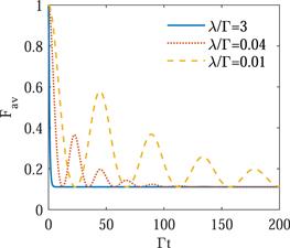
Figure 2. The average fidelity Fav as a function of Γt for different λ/Γ. |
4. Improvement of average fidelity
In this section, two methods are introduced to enhance the average fidelity of our CBRSP protocol. The first method is to perform WMR on some qubits subjected to non-Markovian noise. The second one is to modulate the detuning between the qubit transition frequency and the cavity center frequency.
4.1. Application of quantum measurement reversal
As shown in figure 3, we assume that the entangled sources consisting of the two EPR states ${\left|\psi \right\rangle }_{12}$ and ${\left|\psi \right\rangle }_{34}$ are distributed in dissipative environments to Alice and Bob, and then they make WMR operations on their respective qubits 2 and 4. The reversal operation acting on the single qubit k (k = 2, 4) is given by [40]
$\begin{eqnarray}{R}_{k}=\left(\begin{array}{cc}\sqrt{1-f} & 0\\ 0 & 1\end{array}\right),\end{eqnarray}$
under the basis $\left\{\left|0\right\rangle ,\left|1\right\rangle \right\}$, where the parameter f (0 ≤ f ≤ 1) is the strength of WMR. Moreover, the reversal measurement Rk was demonstrated in experiment with linear optical systems [32, 33].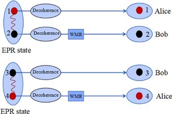
Figure 3. The EPR states are exposed to dissipative environments and qubits 2 and 4 are operated by WMR operations after decoherence. |
Based on the quantum circuit in figure 1, the density matrix of the final output state after the partial measurements reads21 ) (23 ), (27 ), (28 ), the final output state ρout−r and its corresponding average fidelity Fav−r can be derived analytically, and their detailed expressions are described in the appendix .
$\begin{eqnarray}{\rho }_{\mathrm{out}-r}={\mathrm{Tr}}_{{11}^{{\prime} }{33}^{{\prime} }5}\{{U}_{\mathrm{RSP}}[({R}_{2}\otimes {R}_{4})({\rho }_{12}(t)\otimes {\left|0\right\rangle }_{{1}^{{\prime} }}\left\langle 0\right|\otimes {\rho }_{34}(t)\otimes {\left|0\right\rangle }_{{3}^{{\prime} }}\left\langle 0\right|){\left({R}_{2}\otimes {R}_{4}\right)}^{+}\otimes {\left|0\right\rangle }_{5}\left\langle 0\right|]{U}_{\mathrm{RSP}}^{+}\}.\ \end{eqnarray}$
According to equations (Based on the Fav−r expanded in the appendix , in figure 4 we plot the average fidelity assisted by WMR as a function of Γt for different values of λ/Γ. The optimal WMR strength fopt that maximizes the average fidelity versus Γt for the fixed λ/Γ is also shown in the insets of the figure. From the figure, we can see that the average fidelity exhibits different evolution behaviors under the influence of non-Markovian (a) and Markovian (b) regimes. More explicitly, as shown in figure 4(a), the optimal average fidelity ${F}_{\mathrm{av}-r}^{\mathrm{opt}}$ exhibits the oscillation behavior with a damping amplitude similar to the case of the average fidelity Fav−n without WMR. Moreover, with the introduction of the optimal WMR operations on the qubits 2 and 4, the revival amplitude of ${F}_{\mathrm{av}-r}^{\mathrm{opt}}$ increases markedly and its stable value is enhanced to 4/9, larger than the stable value of 1/9 for Fav−n. Furthermore, as shown in figure 4(b), for the given Γt, the value of the optimal average fidelity ${F}_{\mathrm{av}-r}^{\mathrm{opt}}$ in Markovian regime is more than that of Fav−n, and ${F}_{\mathrm{av}-r}^{\mathrm{opt}}$ decays rapidly to the same stable value of 4/9 as the case of non-Markovian regime. Additionally, from the insets of figure 4, one can see that the optimal WMR strength fopt for λ/Γ = 0.01 displays an oscillation behavior, which may be related to the memory effects of non-Markovian environment, while fopt for λ/Γ = 3 increases gradually with the growth of Γt. Therefore, after the WMR with optimal strength, no matter whether our CBRSP scheme is subjected to Markovian or non-Markovian noises, the average fidelity can be remarkably enhanced for any Γt > 0.
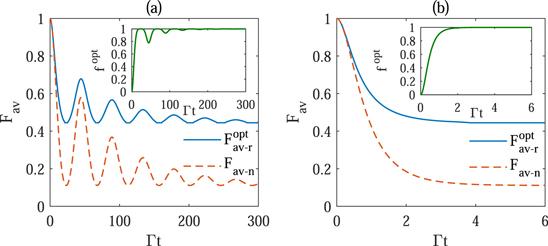
Figure 4. The average fidelities ${F}_{\mathrm{av}-r}^{\mathrm{opt}}$ with optimal WMR and Fav−n without WMR as a function of Γt for (a) λ/Γ = 0.01 and (b) λ/Γ = 3. The insets show the optimal WMR strength fopt corresponding to the average fidelity ${F}_{\mathrm{av}-r}^{\mathrm{opt}}$. |
4.2. Application of detuning modulation
In this section, we turn to examine how to enhance the average fidelity of our CBRSP scheme by adjusting the detuning between the qubit frequency and the cavity center frequency. Detuning modulation is used to generate and protect steady-state entanglement in Markovian [44] and non-Markovian [45] environments. Considering the detuning parameter, the reservoir spectral density of equation (19 ) can be rewritten as [46]
$\begin{eqnarray}J(\omega )=\displaystyle \frac{1}{2\pi }\displaystyle \frac{{\rm{\Gamma }}{\lambda }^{2}}{{\left({\omega }_{0}-\omega -{\rm{\Delta }}\right)}^{2}+{\lambda }^{2}},\end{eqnarray}$
where Δ is the detuning between the atomic transition frequency ω0 and the cavity center frequency ω. Similarly, the corresponding time-dependent function ${\xi }^{{\prime} }\left(t\right)$ takes the form $\begin{eqnarray}{\xi }^{{\prime} }\left(t\right)={{\rm{e}}}^{-(\lambda -{\rm{i}}{\rm{\Delta }})t/2}\left[\cosh \left(\displaystyle \frac{{d}t}{2}\right)+\displaystyle \frac{\lambda -{\rm{i}}{\rm{\Delta }}}{{d}}\sinh \left(\displaystyle \frac{{d}t}{2}\right)\right],\end{eqnarray}$
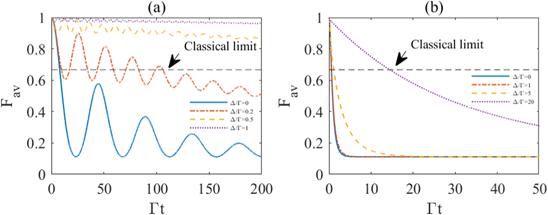
with ${d}=\sqrt{{\left(\lambda -{\rm{i}}{\rm{\Delta }}\right)}^{2}-2\lambda {\rm{\Gamma }}}$.By substituting ${P}^{{\prime} }(t)={\left|{\xi }^{{\prime} }\left(t\right)\right|}^{2}$ for P(t) in equation (26 ), in figure 5 we plot the average fidelity Fav versus Γt with respect to different Δ/Γ and λ/Γ. From figure 5(a), it can be seen that with the increase of Δ/Γ, the average fidelity oscillates more rapidly, i.e., the oscillation period becomes shorter, while the revival amplitude of the average fidelity is greatly enhanced. If the detuning is increased to Δ/Γ = 1, the average fidelity tends to preserve a nearly maximal stationary value of 1. As shown in figure 5(b), the average fidelity in Markovian regime diminishes more slowly with the increasing detuning, and the decay time for the average fidelity from the initial value 1 to the best classically achievable value 2/3 can be remarkably extended. Thereby, whether our CBRSP scheme is in non-Markovian or Markovian regime, the average fidelity can be improved with slow decay for large detuning, especially for the non-Markovian situation. In the case that the EPR states suffer from the dissipative environments, the average fidelity can be preserved for a long time if the non-Markovianity and the detuning conditions are satisfied at the same time.
Figure 5. The average fidelity Fav as a function of Γt for different values of Δ/Γ with (a) λ/Γ = 0.01 and (b) λ/Γ = 3. |
5. Conclusions
In summary, we have investigated deterministic CBRSP of an arbitrary single-qubit state via two EPR states serving as the entanglement source distributed in dissipative environments. The quantum circuit of our protocol is first designed by means of unitary matrix decomposition technique, and then the corresponding average fidelity is derived analytically. Since the quantum circuit of our CBRSP scheme is constructed completely, its experimental implementation may be feasible with the help of IBM Quantum Experience [47, 48]. At this point, our scheme is relatively superior to the previous bidirectional RSP schemes [13–19, 28–30, 37], whose quantum circuits are only partially designed or not. Moreover, we have explored how to improve the average fidelity with the assistance of WMR and detuning modulation. Our results show that the value of average fidelity can be remarkably enhanced through the introduction of the proper WMR. For the large detuning between the qubit frequency and the cavity frequency, the decay rate of the average fidelity is reduced significantly, especially the average fidelity in the non-Markovian regime can be preserved the approximate ideal value of 1 for a long time. Besides, both of the two fidelity enhancement schemes are more effective in non-Markovian situation, due to the memory effects of the environment. Since the non-Markovian dynamics of open systems is a useful feature against detrimental effect of the dissipative environment, there is considerable progress on non-Markovian reservoir engineering in both experiment [49, 50] and theory [51, 52]. We expect that our findings could shed some light on designing efficient quantum communication schemes against environment noises in structured reservoirs.