Welcome to visit Communications in Theoretical Physics,
Mathematical Physics

The unified transform method to the high-order nonlinear Schrödinger equation with periodic initial condition

  • Leilei Liu ,
  • Weiguo Zhang ,
  • Jian Xu ,
  • Yuli Guo
Expand
  • College of Science, University of Shanghai for Science and Technology, China

Received date: 2022-02-19

  Revised date: 2022-05-29

  Accepted date: 2022-06-20

  Online published: 2022-08-01

Copyright

© 2022 Institute of Theoretical Physics CAS, Chinese Physical Society and IOP Publishing

Abstract

In this paper, we study the high-order nonlinear Schrödinger equation with periodic initial conditions via the unified transform method extended by Fokas and Lenells. For the high-order nonlinear Schrödinger equation, the initial value problem on the circle can be expressed in terms of the solution of a Riemann–Hilbert problem. The related jump matrix can be explicitly expressed based on the initial data alone. Furthermore, we present the explicit solution, which corresponds to a one-gap solution.

Cite this article

Leilei Liu , Weiguo Zhang , Jian Xu , Yuli Guo . The unified transform method to the high-order nonlinear Schrödinger equation with periodic initial condition[J]. Communications in Theoretical Physics, 2022 , 74(8) : 085001 . DOI: 10.1088/1572-9494/ac7a23

1. Introduction

For nonlinear partial differential equations, solutions of spatial infinite decay and spatially periodic solutions are the two most widely studied classes of solutions. In the first of these classes, solutions of the initial value problem of integrable evolution equations can be solved by linear operations [1]. To be precise, the inverse scatter transform, which was introduced about half a century ago, solved this problem groundbreakingly [26].
For the above-mentioned second classes-the spatially periodic solution, the finite gap integration method was introduced in the 1970s [7]. Considering rational combinations of theta functions, which are defined on Riemann surfaces that the number of branch cuts is finite, the approach generates exact solutions named finite-gap solutions. If the given initial data belongs to the finite gap class, according to the Jacobian inversion problem on the finite Riemann surface, we can retrieve the solution of the initial value problem. But nevertheless, if the initial data does not belong to the finite gap potential energy category, then an additional theory is needed. Although the method can be extended to infinite Riemann surfaces [810], the solutions of the Jacobian inversion problems on infinite surfaces are quite complicated. In fact, solutions with finite gaps are not easy to obtain computationally [2, 11].
In 1997, Fokas proposed a novel method called the unified transform method (UTM) for solving the initial boundary value problem of integrable systems [12, 13]. The initial boundary value problems of many integrable equations have been studied, such as the nonlinear Schrödinger equation, sine-Gordon equation, and the mKdV equation [1419]. In 2013, Lenells generalized the UTM to the initial boundary value problem of an integrable system with pairs of third-order matrices Lax on the half-line [20]. In 2014, Fan Engui and Xu Jian applied the UTM to the initial boundary value problem on the half-line of the Sasa-Satsuma equation and three-wave equation [21, 22]. Recently, Yan Zhenya extended the UTM to the fourth-order matrix spectral problem [23].
In 2004, Fokas and Its realized the UTM to the nonlinear Schrödinger equation on the finite interval [24]. They show the solution of the nonlinear Schrödinger equation can be obtained by the related Riemann–Hilbert problem involving spectral functions defined in terms of initial datum and boundary values. Facts have proved that the boundary conditions, which correspond to the x-periodic problem, are linearizable. Recently, using the NLS equation as an example, Fokas and Lenells proposed a new method based on the unified transform to obtain the solution of the NLS equation with periodic initial conditions [25, 26]. Their method provides a new perspective on the initial value problem on the circle, and creatively they get the expression of the solution of a Riemann–Hilbert problem only involving the initial data.
For the inverse scattering method, the unified transformation method is a generalization of the initial value problem to the initial boundary value problem. Through the simultaneous spectral analysis of the x-part and the t-part of the Lax pair, the solution of the initial boundary value problem of the integrable equation can be represented by the solution of the matrix RH problem on the complex plane. The jump matrix of the RH problem of the initial boundary value problem can be explicitly expressed by the spectral matrix corresponding to the initial conditions and boundary conditions.
It is well known that the nonlinear Schrödinger equation can well describe the wave evolution in deep water and optical fibers [27, 28]. In addition, the nonlinear Schrödinger equation is also a general model for some multiplicity of nonlinear phenomena in plasma waves, Bose–Einstein condensates, and other physical phenomena [2931]. One of the most important applications is the soliton in optical fibers [32]. Nonetheless, several phenomena can not be described by low order dispersion NLS equation. When considering the propagation of ultrashort pulses through the fiber, that is, pulses less than 100-fs, it has been shown that the model should include high-order dispersion, self-steepening, self-frequency, and high-order effects. The high-order nonlinear Schrödinger equation (1.1) is particularly important for describing the more complex phenomena. In this paper, we study the high-order nonlinear Schrödinger equation
$\begin{eqnarray}\begin{array}{l}{\rm{i}}{q}_{t}+{q}_{{xx}}+2q| q{| }^{2}+{q}_{{xxxx}}+6{{q}_{x}}^{2}\bar{q}+4q| {q}_{x}{| }^{2}\\ \quad +8| q{| }^{2}{q}_{{xx}}+2| q{| }^{2}{\bar{q}}_{{xx}}+6| q{| }^{4}q=0,\end{array}\end{eqnarray}$
suppose q(x, t) is a smooth solution of equation (1.1) for $(x,t)\in {\mathbb{R}}\times [0,\infty )$ which is x-periodic of period L > 0, i.e. q(x + L, t) = q(x, t). We consider the following initial datum involving a single exponential:
$\begin{eqnarray}q(x,0)={q}_{0}{{\rm{e}}}^{\tfrac{2{\rm{i}}\pi N}{L}x},\quad x\in [0,L],\end{eqnarray}$
where N is an integer and the constant q0 > 0. The high-order nonlinear Schrödinger equation has been studied through many methods, such as Darboux Transformation, the Inverse scattering transform and so on [3341]. However, to the best of our knowledge, the high-order nonlinear Schrödinger equation with periodic initial conditions was not reported before. Although we used the same method as in [25, 26], it is worth noting that the RH problem we studied was more complex. It lays the foundation for us to further explore a certain class of nonlinear integrable equations, such as the KdV equation, the mKdV equation, and the Hirota equation.
The outline of this paper is as follows: in section 2, we apply the UTM to a high-order nonlinear Schrödinger equation posed on a finite interval $x\in [0,L]\subset {\mathbb{R}}$. In section 3, the high-order nonlinear Schrödinger equation on the periodic problem with a single exponential initial data $(i.e.q(x,0)={q}_{0}{{\rm{e}}}^{\tfrac{2{\rm{i}}\pi N}{L}x},x\in [0,L])$ was considered. Moreover, by solving the associated RH problem involving the initial datum alone, the exact solution is obtained, which corresponds to the one-gap solution.

2. The UTM to the high-order nonlinear Schrödinger equation on a finite interval

In this section, we apply the UTM to the high-order nonlinear Schrödinger equation with the following data,
$\begin{eqnarray*}\begin{array}{l}q(x,0)={q}_{0}(x),\quad x\in [0,L],\\ q(0,t),{q}_{x}(0,t),{q}_{{xx}}(0,t),{q}_{{xxx}}(0,t),q(L,t),\\ {q}_{x}(L,t),{q}_{{xx}}(L,t),{q}_{{xxx}}(L,t),\quad t\in [0,T].\end{array}\end{eqnarray*}$
According to the AKNS formalism, the high-order nonlinear Schrödinger equation has a lax pair given by
$\begin{eqnarray}\left\{\begin{array}{l}{{\rm{\Psi }}}_{x}+{\rm{i}}\lambda [{\sigma }_{3},{\rm{\Psi }}]=Q{\rm{\Psi }},\\ {{\rm{\Psi }}}_{t}+{\rm{i}}(2{\lambda }^{2}-8{\lambda }^{4})[{\sigma }_{3},{\rm{\Psi }}]=V{\rm{\Psi }},\end{array}\right.\end{eqnarray}$
with
$\begin{eqnarray*}\begin{array}{rcl}V & = & {\rm{i}}{V}_{3}{\lambda }^{3}+{\rm{i}}{V}_{2}{\lambda }^{2}+{\rm{i}}{V}_{1}\lambda +{\rm{i}}{V}_{0},\\ {V}_{0} & = & (6{Q}^{2}-{Q}_{x}-{Q}_{{xxx}}+{Q}_{x}^{2}+3{Q}^{4}-{{QQ}}_{{xx}}-{Q}_{{xx}}Q){\sigma }_{3},\\ {V}_{1} & = & 2{\rm{i}}(-{{QQ}}_{x}+{Q}_{x}Q-Q+2{Q}^{3}-{Q}_{{xx}}),\\ {V}_{2} & = & (4{Q}^{2}+4{Q}_{x}){\sigma }_{3},{V}_{3}=8{\rm{i}}Q,\end{array}\end{eqnarray*}$
where $\Psi$(x, t, λ) is a 2 × 2 matrix-valued function, $\lambda \in {\mathbb{C}}$ is an auxiliary (spectra) parameter, the potential matrix Q and σ3 are defined by
$\begin{eqnarray}Q=\left(\begin{array}{cc}0 & q(x,t)\\ -\bar{q}(x,t) & 0\end{array}\right),{\sigma }_{3}=\left(\begin{array}{cc}1 & 0\\ 0 & -1\end{array}\right),\end{eqnarray}$
the W(x, t, λ) and θ are defined by $W(x,t,\lambda )\,={{\rm{e}}}^{{\rm{i}}\theta \hat{{\sigma }_{3}}}(Q{\rm{\Psi }}{\rm{d}}x+V{\rm{\Psi }}{\rm{d}}t),\theta =\lambda x+(2{\lambda }^{2}-8{\lambda }^{4})t.$ According to equation (2.1), we get
$\begin{eqnarray}{\rm{\Psi }}(x,t,\lambda )=I+{\int }_{({x}_{* },{t}_{* })}^{(x,t)}{{\rm{e}}}^{-{\rm{i}}\theta \hat{{\sigma }_{3}}}W(y,\tau ,\lambda ),\end{eqnarray}$
where (x*, t*) ∈ [0, L] × [0, T] is an arbitrary point and integral means the line integral that smoothly connects the indicated points. We choose the point (x*, t*) as each of the corners of the polygonal domain. Therefore we define four solutions $\Psi$1, $\Psi$2, $\Psi$3, $\Psi$4, corresponding to the four points (0, T), (0, 0), (L, 0), (L, T).
$\begin{eqnarray}\begin{array}{l}{{\rm{\Psi }}}_{1}(x,t,\lambda )=I+{\displaystyle \int }_{0}^{x}{{\rm{e}}}^{-{\rm{i}}\lambda (x-y)\hat{{\sigma }_{3}}}(Q{{\rm{\Psi }}}_{1})(y,t,\lambda ){\rm{d}}y-{{\rm{e}}}^{-{\rm{i}}\lambda x\hat{{\sigma }_{3}}}\\ \quad \times {\displaystyle \int }_{t}^{T}{{\rm{e}}}^{-{\rm{i}}(2{\lambda }^{2}-8{\lambda }^{4})(t-\tau )\hat{{\sigma }_{3}}}(V{{\rm{\Psi }}}_{1})(0,\tau ,\lambda ){\rm{d}}\tau ,\end{array}\end{eqnarray}$
$\begin{eqnarray}\begin{array}{l}{{\rm{\Psi }}}_{2}(x,t,\lambda )=I+{\displaystyle \int }_{0}^{x}{{\rm{e}}}^{-{\rm{i}}\lambda (x-y)\hat{{\sigma }_{3}}}(Q{{\rm{\Psi }}}_{2})(y,t,\lambda ){\rm{d}}y+{{\rm{e}}}^{-{\rm{i}}\lambda x\hat{{\sigma }_{3}}}\\ \quad \times {\displaystyle \int }_{0}^{t}{{\rm{e}}}^{-{\rm{i}}(2{\lambda }^{2}-8{\lambda }^{4})(t-\tau )\hat{{\sigma }_{3}}}(V{{\rm{\Psi }}}_{2})(0,\tau ,\lambda ){\rm{d}}\tau ,\end{array}\end{eqnarray}$
$\begin{eqnarray}\begin{array}{l}{{\rm{\Psi }}}_{3}(x,t,\lambda )=I-{\displaystyle \int }_{x}^{L}{{\rm{e}}}^{-{\rm{i}}\lambda (x-y)\hat{{\sigma }_{3}}}(Q{{\rm{\Psi }}}_{3})(y,t,\lambda ){\rm{d}}y\\ \quad +{{\rm{e}}}^{-{\rm{i}}\lambda (x-L)\hat{{\sigma }_{3}}}\\ \quad \times {\displaystyle \int }_{0}^{t}{{\rm{e}}}^{-{\rm{i}}(2{\lambda }^{2}-8{\lambda }^{4})(t-\tau )\hat{{\sigma }_{3}}}(V{{\rm{\Psi }}}_{3})(L,\tau ,\lambda ){\rm{d}}\tau ,\end{array}\end{eqnarray}$
$\begin{eqnarray}\begin{array}{l}{{\rm{\Psi }}}_{4}(x,t,\lambda )=I-{\int }_{x}^{L}{{\rm{e}}}^{-{\rm{i}}\lambda (x-y)\hat{{\sigma }_{3}}}(Q{{\rm{\Psi }}}_{4})(y,t,\lambda ){\rm{d}}y\\ \quad -{{\rm{e}}}^{-{\rm{i}}\lambda (x-L)\hat{{\sigma }_{3}}}{\int }_{t}^{T}{{\rm{e}}}^{-{\rm{i}}(2{\lambda }^{2}-8{\lambda }^{4})(t-\tau )\hat{{\sigma }_{3}}}(V{{\rm{\Psi }}}_{4})(L,\tau ,\lambda ){\rm{d}}\tau .\end{array}\end{eqnarray}$
Further, we can show that $\Psi$j(x, t, λ), j = 1, 2, 3, 4 satisfies the following bounded and analytic properties in the complex λ plane
$\begin{eqnarray}\begin{array}{l}{[{{\rm{\Psi }}}_{2}]}_{1},{[{{\rm{\Psi }}}_{4}]}_{2}:\quad {D}_{1},\quad {[{{\rm{\Psi }}}_{1}]}_{1},{[{{\rm{\Psi }}}_{3}]}_{2}:\quad {D}_{2},\\ \quad {[{{\rm{\Psi }}}_{3}]}_{1},{[{{\rm{\Psi }}}_{1}]}_{2}:\quad {D}_{3},\quad {[{{\rm{\Psi }}}_{4}]}_{1},{[{{\rm{\Psi }}}_{2}]}_{2}:\quad {D}_{4},\end{array}\end{eqnarray}$
where [A]1 and [A]2 denote the first and second columns of a matrix A, respectively. The Dj (j = 1, ⋯ ,4) is defined as follows
$\begin{eqnarray*}\begin{array}{rcl}{D}_{1} & = & \{\lambda \in {\mathbb{C}}:\mathrm{Im}\lambda \geqslant 0,\mathrm{Re}\lambda [1-8{\left(\mathrm{Re}\lambda \right)}^{2}\\ & & +8{\left(\mathrm{Im}\lambda \right)}^{2}]\geqslant 0\},\\ {D}_{2} & = & \{\lambda \in {\mathbb{C}}:\mathrm{Im}\lambda \geqslant 0,\mathrm{Re}\lambda [1-8{\left(\mathrm{Re}\lambda \right)}^{2}\\ & & +8{\left(\mathrm{Im}\lambda \right)}^{2}]\leqslant 0\},\\ {D}_{3} & = & \{\lambda \in {\mathbb{C}}:\mathrm{Im}\lambda \leqslant 0,\mathrm{Re}\lambda [1-8{\left(\mathrm{Re}\lambda \right)}^{2}\\ & & +8{\left(\mathrm{Im}\lambda \right)}^{2}]\leqslant 0\},\\ {D}_{4} & = & \{\lambda \in {\mathbb{C}}:\mathrm{Im}\lambda \leqslant 0,\mathrm{Re}\lambda [1-8{\left(\mathrm{Re}\lambda \right)}^{2}\\ & & +8{\left(\mathrm{Im}\lambda \right)}^{2}]\geqslant 0\}.\end{array}\end{eqnarray*}$
Note that all the $\Psi$j are entire functions of λ, since the matrices Q and V are traceless, thus we have
$\begin{eqnarray*}\begin{array}{rcl}\det {{\rm{\Psi }}}_{j}(x,t,\lambda ) & = & 1,\quad j=1,\cdots ,4,\\ {{\rm{\Psi }}}_{j}(x,t,\lambda ) & = & I+O\left(\displaystyle \frac{1}{\lambda }\right),\quad \lambda \to \infty .\end{array}\end{eqnarray*}$
The asymptotics here and later are in the corresponding domains of boundedness. See figure 1 for details.
Figure 1. Since our analytical region here is different from [25, 26], we draw the integrable region and the direction of the integration curve for the RH problem according to the definition of Dj, as shown in figure 1. The jump matrices J1, ⋯, J4 are defined in (2.25).
The eigenfunctions $\Psi$j are related by the equations
$\begin{eqnarray}{{\rm{\Psi }}}_{3}(x,t,\lambda )={{\rm{\Psi }}}_{2}(x,t,\lambda ){{\rm{e}}}^{-{\rm{i}}\theta \hat{{\sigma }_{3}}}s(\lambda ),\end{eqnarray}$
$\begin{eqnarray}{{\rm{\Psi }}}_{1}(x,t,\lambda )={{\rm{\Psi }}}_{2}(x,t,\lambda ){{\rm{e}}}^{-{\rm{i}}\theta \hat{{\sigma }_{3}}}S(\lambda ),\end{eqnarray}$
$\begin{eqnarray}{{\rm{\Psi }}}_{4}(x,t,\lambda )={{\rm{\Psi }}}_{3}(x,t,\lambda ){{\rm{e}}}^{-{\rm{i}}(\theta -\lambda L)\hat{{\sigma }_{3}}}{S}_{L}(\lambda ).\end{eqnarray}$
Through the above equation, we get
$\begin{eqnarray*}\begin{array}{rcl}s(\lambda ) & = & {{\rm{\Psi }}}_{3}(0,0,\lambda ),\\ S(\lambda ) & = & {{\rm{\Psi }}}_{1}(0,0,\lambda ),\\ {S}_{L}(\lambda ) & = & {{\rm{\Psi }}}_{4}(L,0,\lambda ).\end{array}\end{eqnarray*}$
Meanwhile, equations (2.9) and (2.11) imply
$\begin{eqnarray}{{\rm{\Psi }}}_{4}(x,t,\lambda )={{\rm{\Psi }}}_{2}(x,t,\lambda ){{\rm{e}}}^{-{\rm{i}}\theta \hat{{\sigma }_{3}}}(s(\lambda ){{\rm{e}}}^{{\rm{i}}\lambda L\hat{{\sigma }_{3}}}{S}_{L}(\lambda )).\end{eqnarray}$
When x = 0, t = T, from equation (2.10), we find $S(\lambda )\,={\left({{\rm{e}}}^{{\rm{i}}(2{\lambda }^{2}-8{\lambda }^{4})T\hat{{\sigma }_{3}}}{{\rm{\Psi }}}_{2}(0,T,\lambda )\right)}^{-1}$. Evaluating equation (2.12) at the point (0, T) and writing $\Psi$2(0, T, λ) in terms of S(λ), we find
$\begin{eqnarray}{{\rm{\Psi }}}_{4}(0,T,\lambda )={{\rm{e}}}^{-{\rm{i}}(2{\lambda }^{2}-8{\lambda }^{4})T\hat{{\sigma }_{3}}}({S}^{-1}(\lambda )s(\lambda ){{\rm{e}}}^{{\rm{i}}\lambda L\hat{{\sigma }_{3}}}{S}_{L}(\lambda )).\end{eqnarray}$
Multiplying equation (2.13) by ${{\rm{e}}}^{{\rm{i}}(2{\lambda }^{2}-8{\lambda }^{4})T\hat{{\sigma }_{3}}}$ and using equation (2.7), we get
$\begin{eqnarray}\begin{array}{l}-I+{S}^{-1}s({{\rm{e}}}^{{\rm{i}}\lambda L\hat{{\sigma }_{3}}}{S}_{L})+{{\rm{e}}}^{{\rm{i}}(2{\lambda }^{2}-8{\lambda }^{4})T\hat{{\sigma }_{3}}}\\ \quad \times {\displaystyle \int }_{0}^{L}{{\rm{e}}}^{{\rm{i}}\lambda y\hat{{\sigma }_{3}}}(Q{{\rm{\Psi }}}_{4})(y,T,\lambda ){\rm{d}}y=0.\end{array}\end{eqnarray}$
The (1, 2)th element of above equation is
$\begin{eqnarray}\begin{array}{l}(a{ \mathcal A }-\bar{b}{{\rm{e}}}^{2{\rm{i}}\lambda L}{ \mathcal B })B-(b{ \mathcal A }+\bar{a}{{\rm{e}}}^{2{\rm{i}}\lambda L}{ \mathcal B })A\\ \quad ={{\rm{e}}}^{2{\rm{i}}(2{\lambda }^{2}-8{\lambda }^{4})T}{c}^{+}(\lambda ),\end{array}\end{eqnarray}$
where
$\begin{eqnarray}{c}^{+}(\lambda )=O\left(\displaystyle \frac{1}{\lambda }\right)+O\left(\displaystyle \frac{{{\rm{e}}}^{2{\rm{i}}\lambda L}}{\lambda }\right),\quad \lambda \to \infty .\end{eqnarray}$
According to symmetry properties, we have
$\begin{eqnarray}\begin{array}{rcl}s(\lambda ) & = & \left(\begin{array}{cc}\bar{a}(\lambda ) & b(\lambda )\\ -\bar{b}(\lambda ) & b(\lambda )\end{array}\right),S(\lambda )=\left(\begin{array}{cc}\bar{A}(\lambda ) & B(\lambda )\\ -\bar{B}(\lambda ) & A(\lambda )\end{array}\right),\\ {S}_{L}(\lambda ) & = & \left(\begin{array}{cc}\bar{{ \mathcal A }}(\lambda ) & { \mathcal B }(\lambda )\\ -\bar{{ \mathcal B }}(\lambda ) & { \mathcal A }(\lambda )\end{array}\right).\end{array}\end{eqnarray}$
Here, and in what follows, a bar over a function denotes that the complex conjugate is taken, not only of the function but also of its argument; this is called the Schwarz conjugate. We can easily get the following properties:
$\begin{eqnarray}\begin{array}{rcl}a\bar{a}+b\bar{b} & = & 1,\quad A\bar{A}+B\bar{B}=1,\\ { \mathcal A }\bar{{ \mathcal A }}+{ \mathcal B }\bar{{ \mathcal B }} & = & 1,\end{array}\end{eqnarray}$
$\begin{eqnarray}\begin{array}{rcl}a(\lambda ) & = & 1+O\left(\displaystyle \frac{1}{\lambda }\right)+O\left(\displaystyle \frac{{{\rm{e}}}^{2{\rm{i}}\lambda L}}{\lambda }\right),\\ b(\lambda ) & = & O\left(\displaystyle \frac{1}{\lambda }\right)+O\left(\displaystyle \frac{{{\rm{e}}}^{2{\rm{i}}\lambda L}}{\lambda }\right),\quad \lambda \to \infty ,\end{array}\end{eqnarray}$
$\begin{eqnarray}\begin{array}{rcl}A(\lambda ) & = & 1+O\left(\displaystyle \frac{1}{\lambda }\right)+O\left(\displaystyle \frac{{{\rm{e}}}^{2{\rm{i}}(2{\lambda }^{2}-8{\lambda }^{4})T}}{\lambda }\right),\\ B(\lambda ) & = & O\left(\displaystyle \frac{1}{\lambda }\right)+O\left(\displaystyle \frac{{{\rm{e}}}^{2{\rm{i}}(2{\lambda }^{2}-8{\lambda }^{4})T}}{\lambda }\right),\quad \lambda \to \infty .\end{array}\end{eqnarray}$
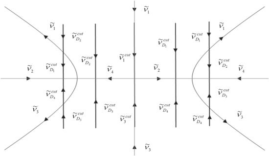
Figure 2. The contour $\tilde{{\rm{\Sigma }}}$ in the complex λ-plane and the associated jump matrices for RH problem for $\tilde{m}$.
Now we construct the RH problem for M(x, t, λ)
$\begin{eqnarray}M=\left\{\begin{array}{ll}\left(\displaystyle \frac{{[{{\rm{\Psi }}}_{2}]}_{1}}{\alpha },{[{{\rm{\Psi }}}_{4}]}_{2}\right),\quad & \lambda \in {D}_{1},\\ \left(\displaystyle \frac{{[{{\rm{\Psi }}}_{1}]}_{1}}{d},{[{{\rm{\Psi }}}_{3}]}_{2}\right),\quad & \lambda \in {D}_{2},\\ \left({[{{\rm{\Psi }}}_{3}]}_{1},\displaystyle \frac{{[{{\rm{\Psi }}}_{1}]}_{2}}{\bar{d}}\right),\quad & \lambda \in {D}_{3},\\ \left({[{{\rm{\Psi }}}_{4}]}_{1},\displaystyle \frac{{[{{\rm{\Psi }}}_{2}]}_{2}}{\bar{\alpha }}\right),\quad & \lambda \in {D}_{4}.\end{array}\right.\end{eqnarray}$
The M satisfies
$\begin{eqnarray}{M}_{-}(x,t,\lambda )={M}_{+}(x,t,\lambda )J(x,t,\lambda ),\lambda \in {\rm{\Sigma }},\end{eqnarray}$
$\begin{eqnarray}M(x,t,\lambda )=I+O(\displaystyle \frac{1}{\lambda }),\lambda \to \infty ,\end{eqnarray}$
where
$\begin{eqnarray}{\rm{\Sigma }}={{\rm{\Sigma }}}_{1}\cup {{\rm{\Sigma }}}_{2}\cup {{\rm{\Sigma }}}_{3}\cup {{\rm{\Sigma }}}_{4},\end{eqnarray}$
$\begin{eqnarray*}\begin{array}{rcl}{{\rm{\Sigma }}}_{1} & = & \{\lambda \in {\mathbb{C}}:\arg \lambda =\displaystyle \frac{\pi }{2}\}\cup \{\lambda \in {\mathbb{C}}:\mathrm{Im}\lambda \geqslant 0,1\\ & & -8{\left(\mathrm{Re}\lambda \right)}^{2}+8{\left(\mathrm{Im}\lambda \right)}^{2}=0\},\\ {{\rm{\Sigma }}}_{2} & = & \{\lambda \in {\mathbb{C}}:\mathrm{Im}\lambda =0,-\infty \lt \mathrm{Re}\lambda \leqslant -\displaystyle \frac{\sqrt{2}}{4}\}\cup \\ & & \{\lambda \in {\mathbb{C}}:\mathrm{Im}\lambda =0,0\leqslant \mathrm{Re}\lambda \leqslant \displaystyle \frac{\sqrt{2}}{4}\},\\ {{\rm{\Sigma }}}_{3} & = & \{\lambda \in {\mathbb{C}}:\arg \lambda =\displaystyle \frac{3\pi }{2}\}\cup \{\lambda \in {\mathbb{C}}:\mathrm{Im}\lambda \leqslant 0,1\\ & & -8{\left(\mathrm{Re}\lambda \right)}^{2}+8{\left(\mathrm{Im}\lambda \right)}^{2}=0\},\\ {{\rm{\Sigma }}}_{4} & = & \{\lambda \in {\mathbb{C}}:\mathrm{Im}\lambda =0,\displaystyle \frac{\sqrt{2}}{4}\leqslant \mathrm{Re}\lambda \lt +\infty \}\cup \\ & & \{\lambda \in {\mathbb{C}}:\mathrm{Im}\lambda =0,-\displaystyle \frac{\sqrt{2}}{4}\leqslant \mathrm{Re}\lambda \leqslant 0\},\end{array}\end{eqnarray*}$
and the jump matrix J is defined by
$\begin{eqnarray}J=\left\{\begin{array}{l}{J}_{1}=\left(\begin{array}{cc}\displaystyle \frac{\delta }{d} & -{ \mathcal B }{{\rm{e}}}^{2{\rm{i}}\lambda L}{{\rm{e}}}^{-2{\rm{i}}\theta }\\ \displaystyle \frac{-\bar{B}{{\rm{e}}}^{2{\rm{i}}\theta }}{d\alpha } & \displaystyle \frac{a}{\alpha }\end{array}\right),\quad \lambda \in {{\rm{\Sigma }}}_{1},\\ {J}_{2}=\left(\begin{array}{cc}1 & -\displaystyle \frac{\beta {{\rm{e}}}^{-2{\rm{i}}\theta }}{\bar{\alpha }}\\ \displaystyle \frac{-\bar{\beta }{{\rm{e}}}^{2{\rm{i}}\theta }}{\alpha } & \displaystyle \frac{1}{\alpha \bar{\alpha }}\end{array}\right),\quad \lambda \in {{\rm{\Sigma }}}_{2},\\ {J}_{3}=\left(\begin{array}{cc}\displaystyle \frac{\bar{\delta }}{\bar{d}} & -\displaystyle \frac{B{{\rm{e}}}^{-2{\rm{i}}\theta }}{\bar{d}\bar{\alpha }}\\ -\bar{{ \mathcal B }}{{\rm{e}}}^{-2{\rm{i}}\lambda L}{{\rm{e}}}^{2{\rm{i}}\theta } & \displaystyle \frac{\bar{a}}{\bar{\alpha }}\end{array}\right),\quad \lambda \in {{\rm{\Sigma }}}_{3},\\ {J}_{4}={J}_{3}{J}_{2}^{-1}{J}_{1},\quad \lambda \in {{\rm{\Sigma }}}_{4},\end{array}\right.\end{eqnarray}$
where
$\begin{eqnarray}\begin{array}{rcl}\alpha (\lambda ) & = & a{ \mathcal A }-\bar{b}{ \mathcal B }{{\rm{e}}}^{2{\rm{i}}\lambda L},\\ \beta (\lambda ) & = & b{ \mathcal A }+\bar{a}{ \mathcal B }{{\rm{e}}}^{2{\rm{i}}\lambda L},\\ d(\lambda ) & = & a\bar{A}+b\bar{B},\quad \delta (\lambda )=\alpha \bar{A}+\beta \bar{B}.\end{array}\end{eqnarray}$
The solution q(x, t) of equation (1.1) can be recovered from
$\begin{eqnarray}q(x,t)=2{\rm{i}}\mathop{\mathrm{lim}}\limits_{\lambda \to \infty }\lambda {M}_{12}(x,t,\lambda ).\end{eqnarray}$
Note that jump matrix J depends on the initial datum q(x, 0) and the boundary values q(0, t), qx(0, t), qxx(0, t), qxxx(0, t), q(L, t), qx(L, t), qxx(L, t), qxxx(L, t). If all values are known, we can obtain the q(x, t) via the solution of the RH problem.

3. The high-order nonlinear Schrödinger equation on the periodic problem with a single exponential initial data

Suppose q(x, t) is a smooth solution of equation (1.1) for $(x,t)\in {\mathbb{R}}\times [0,\infty )$ which is x-periodic of period L > 0, i.e. q(x + L, t) = q(x, t). We consider the following initial datum involving a single exponential:
$\begin{eqnarray}q(x,0)={q}_{0}{{\rm{e}}}^{\tfrac{2{\rm{i}}\pi N}{L}x},\quad x\in [0,L],\end{eqnarray}$
where N is an integer and the constant q0 > 0. In this case, we clearly have ${ \mathcal A }=A$ and ${ \mathcal B }=B$. Therefore the jump matrices Ji defined in equation (2.25) become
$\begin{eqnarray}\begin{array}{rcl}{J}_{1} & = & \left(\begin{array}{cc}\displaystyle \frac{\delta }{d} & -B{{\rm{e}}}^{2{\rm{i}}\lambda L}{{\rm{e}}}^{-2{\rm{i}}\theta }\\ \displaystyle \frac{-\bar{B}{{\rm{e}}}^{2{\rm{i}}\theta }}{d\alpha } & \displaystyle \frac{a}{\alpha }\end{array}\right),\quad {J}_{2}=\left(\begin{array}{cc}1 & -\displaystyle \frac{\beta {{\rm{e}}}^{-2{\rm{i}}\theta }}{\bar{\alpha }}\\ \displaystyle \frac{-\bar{\beta }{{\rm{e}}}^{2{\rm{i}}\theta }}{\alpha } & \displaystyle \frac{1}{\alpha \bar{\alpha }}\end{array}\right),\\ {J}_{3} & = & \left(\begin{array}{cc}\displaystyle \frac{\bar{\delta }}{\bar{d}} & -\displaystyle \frac{B{{\rm{e}}}^{-2{\rm{i}}\theta }}{\bar{d}\bar{\alpha }}\\ -\bar{B}{{\rm{e}}}^{-2{\rm{i}}\lambda L}{{\rm{e}}}^{2{\rm{i}}\theta } & \displaystyle \frac{\bar{a}}{\bar{\alpha }}\end{array}\right),\quad {J}_{4}={J}_{3}{J}_{2}^{-1}{J}_{1},\end{array}\end{eqnarray}$
where
$\begin{eqnarray}\begin{array}{rcl}\alpha (\lambda ) & = & {aA}-\bar{b}B{{\rm{e}}}^{2{\rm{i}}\lambda L},\quad \beta (\lambda )={bA}+\bar{a}B{{\rm{e}}}^{2{\rm{i}}\lambda L},\\ d(\lambda ) & = & a\bar{A}+b\bar{B},\quad \delta (\lambda )=\alpha \bar{A}+\beta \bar{B}.\end{array}\end{eqnarray}$
Similarly, we have
$\begin{eqnarray}s(\lambda )=\left(\begin{array}{cc}\bar{a}(\lambda ) & b(\lambda )\\ -\bar{b}(\lambda ) & b(\lambda )\end{array}\right),\quad S(\lambda )=\left(\begin{array}{cc}\bar{A}(\lambda ) & B(\lambda )\\ -\bar{B}(\lambda ) & A(\lambda )\end{array}\right),\end{eqnarray}$
where
$\begin{eqnarray}s(\lambda )={{\rm{\Psi }}}_{3}(0,0,\lambda ),\quad S(\lambda )={{\rm{\Psi }}}_{1}(0,0,\lambda ).\end{eqnarray}$
Clearly, S(λ) depends on T, while s(λ) does not. We have the global relation:
$\begin{eqnarray}\begin{array}{l}({aA}-\bar{b}{{\rm{e}}}^{2{\rm{i}}\lambda L}B)B-({bA}+\bar{a}{{\rm{e}}}^{2{\rm{i}}\lambda L}B)A\\ \quad ={{\rm{e}}}^{2{\rm{i}}(2{\lambda }^{2}-8{\lambda }^{4})T}{c}^{+}(\lambda ),\end{array}\end{eqnarray}$
where
$\begin{eqnarray}{c}^{+}(\lambda )=O\left(\displaystyle \frac{1}{\lambda }\right)+O\left(\displaystyle \frac{{{\rm{e}}}^{2{\rm{i}}\lambda L}}{\lambda }\right),\quad \lambda \to \infty .\end{eqnarray}$
Meanwhile, a, b, A, B satisfy the equation (2.18), equation (2.19) and equation (2.20). According to equation (2.27), the solution q(x, t) of equation (1.1) can be recovered by
$\begin{eqnarray}q(x,t)=2{\rm{i}}\mathop{\mathrm{lim}}\limits_{\lambda \to \infty }\lambda {M}_{12}(x,t,\lambda ).\end{eqnarray}$

3.1. The RH problem for m
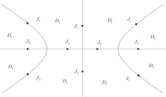
It can be formulated, which involves an RH problem where the ratio Γ = B/A is used to define the matrix jump, relative to A and B. Now we consider the piecewise meromorphic function m(x, t, k) defined by
$\begin{eqnarray}m=\left\{\begin{array}{l}\left(\displaystyle \frac{A{[{{\rm{\Psi }}}_{2}]}_{1}}{\alpha },\displaystyle \frac{{[{{\rm{\Psi }}}_{4}]}_{2}}{A}\right),\quad \lambda \in {D}_{1},\\ \left(\displaystyle \frac{{[{{\rm{\Psi }}}_{1}]}_{1}}{d},{[{{\rm{\Psi }}}_{3}]}_{2}\right),\quad \lambda \in {D}_{2},\\ \left({[{{\rm{\Psi }}}_{3}]}_{1},\displaystyle \frac{{[{{\rm{\Psi }}}_{1}]}_{2}}{\bar{d}}\right),\quad \lambda \in {D}_{3},\\ \left(\displaystyle \frac{{[{{\rm{\Psi }}}_{4}]}_{1}}{\bar{A}},\displaystyle \frac{\bar{A}{[{{\rm{\Psi }}}_{2}]}_{2}}{\bar{\alpha }}\right),\quad \lambda \in {D}_{4}.\end{array}\right.\end{eqnarray}$
The relationship between functions m and M defined in equation (2.21) is as follows:
$\begin{eqnarray}m={MH},\end{eqnarray}$
where the piecewise meromorphic function H is defined by
$\begin{eqnarray}\begin{array}{rcl}{H}_{1} & = & \left(\begin{array}{cc}A & 0\\ 0 & \displaystyle \frac{1}{A}\end{array}\right),\quad {H}_{2}={H}_{3}=I,\\ {H}_{4} & = & \left(\begin{array}{cc}\displaystyle \frac{1}{\bar{A}} & 0\\ 0 & \bar{A}\end{array}\right),\end{array}\end{eqnarray}$
where Hj is defined in the region Dj, j = 1, ⋯ ,4.
We can get a RH problem for m as follows:

m(x, t, λ) is analytic in ${\mathbb{C}}\setminus {\rm{\Sigma }}$, and continuous on ${\rm{\Sigma }}\setminus \{0,\pm \tfrac{\sqrt{2}}{4}\}$.

m(x, t, λ)=m+(x, t, λ)&ugr;(x, t, λ), λ ∈ Σ$\setminus \{0,\pm \tfrac{\sqrt{2}}{4}\}$.

$m(x,t,\lambda )=I\,+\,O(\tfrac{1}{\lambda }),\quad \lambda \to \infty $.

m(x, t, λ) = O(1) λ → 0.

The jump matrix &ugr;(x, t, λ) is defined by
$\begin{eqnarray}\begin{array}{l}{\upsilon }_{1}=\left(\begin{array}{cc}\displaystyle \frac{a+b\bar{{\rm{\Gamma }}}+{\rm{\Gamma }}(\bar{a}\bar{{\rm{\Gamma }}}-\bar{b}){{\rm{e}}}^{2{\rm{i}}\lambda L}}{a+b\bar{{\rm{\Gamma }}}} & -{\rm{\Gamma }}{{\rm{e}}}^{2{\rm{i}}\lambda L}{{\rm{e}}}^{-2{\rm{i}}\theta }\\ \displaystyle \frac{-\bar{{\rm{\Gamma }}}{{\rm{e}}}^{2{\rm{i}}\theta }}{(a+b\bar{{\rm{\Gamma }}})(a-\bar{b}{\rm{\Gamma }}{{\rm{e}}}^{2{\rm{i}}\lambda L})} & \displaystyle \frac{a}{a-\bar{b}{\rm{\Gamma }}{{\rm{e}}}^{2{\rm{i}}\lambda L}}\end{array}\right),\\ \quad \lambda \in {{\rm{\Sigma }}}_{1},\\ {\upsilon }_{2}=\left(\begin{array}{cc}1+{\rm{\Gamma }}\bar{{\rm{\Gamma }}} & \displaystyle \frac{-(\bar{a}{\rm{\Gamma }}{{\rm{e}}}^{2{\rm{i}}\lambda L}+b){{\rm{e}}}^{-2{\rm{i}}\theta }}{\bar{a}-b\bar{{\rm{\Gamma }}}{{\rm{e}}}^{-2{\rm{i}}\lambda L}}\\ \displaystyle \frac{-(\bar{b}+{{\rm{e}}}^{-2{\rm{i}}\lambda L}a\bar{{\rm{\Gamma }}}){{\rm{e}}}^{2{\rm{i}}\theta }}{a-{{\rm{e}}}^{2{\rm{i}}\lambda L}\bar{b}{\rm{\Gamma }}} & \displaystyle \frac{1}{(a-\bar{b}{\rm{\Gamma }}{{\rm{e}}}^{2{\rm{i}}\lambda L})(\bar{a}-b\bar{{\rm{\Gamma }}}{{\rm{e}}}^{-2{\rm{i}}\lambda L})}\end{array}\right),\\ \quad \lambda \in {{\rm{\Sigma }}}_{2},\\ {\upsilon }_{3}=\left(\begin{array}{cc}\displaystyle \frac{\bar{a}+\bar{b}{\rm{\Gamma }}+\bar{{\rm{\Gamma }}}(a{\rm{\Gamma }}-b){{\rm{e}}}^{-2{\rm{i}}\lambda L}}{\bar{a}+\bar{b}{\rm{\Gamma }}} & -\displaystyle \frac{{\rm{\Gamma }}{{\rm{e}}}^{-2{\rm{i}}\theta }}{(\bar{a}+\bar{b}{\rm{\Gamma }})(\bar{a}-b\bar{{\rm{\Gamma }}}{{\rm{e}}}^{-2{\rm{i}}\lambda L})}\\ -\bar{{\rm{\Gamma }}}{{\rm{e}}}^{-2{\rm{i}}\lambda L}{{\rm{e}}}^{2{\rm{i}}\theta } & \displaystyle \frac{\bar{a}}{\bar{a}-b\bar{{\rm{\Gamma }}}{{\rm{e}}}^{-2{\rm{i}}\lambda L}}\end{array}\right),\\ \quad \lambda \in {{\rm{\Sigma }}}_{3},\\ {\upsilon }_{4}=\left(\begin{array}{cc}\displaystyle \frac{1+{\rm{\Gamma }}\bar{{\rm{\Gamma }}}}{(a+b\bar{{\rm{\Gamma }}})(\bar{a}+\bar{b}{\rm{\Gamma }})} & \displaystyle \frac{(b-a{\rm{\Gamma }}){{\rm{e}}}^{-2{\rm{i}}\theta }}{\bar{a}+\bar{b}{\rm{\Gamma }}}\\ \displaystyle \frac{(\bar{b}-\bar{a}\bar{{\rm{\Gamma }}}){{\rm{e}}}^{2{\rm{i}}\theta }}{a+b\bar{{\rm{\Gamma }}}} & 1\end{array}\right),\\ \quad \lambda \in {{\rm{\Sigma }}}_{4}.\end{array}\end{eqnarray}$
Furthermore, the function m admit the symmetry relations
$\begin{eqnarray}\begin{array}{rcl}{m}_{11}(x,t,\lambda ) & = & {\bar{m}}_{22}(x,t,\bar{\lambda }),\\ {m}_{21}(x,t,\lambda ) & = & -{\bar{m}}_{12}(x,t,\bar{\lambda }).\end{array}\end{eqnarray}$

3.2. The RH problem for $\tilde{m}$

We defined the function $\tilde{{\rm{\Gamma }}}$ by
$\begin{eqnarray}\tilde{{\rm{\Gamma }}}=-\displaystyle \frac{1}{2{{\rm{e}}}^{{\rm{i}}\lambda L}\bar{b}}(\bar{a}{{\rm{e}}}^{{\rm{i}}\lambda L}-a{{\rm{e}}}^{-{\rm{i}}\lambda L}-{\rm{i}}\sqrt{4-{\bigtriangleup }^{2}}),\end{eqnarray}$
where △(λ) is given by
$\begin{eqnarray}\bigtriangleup =a{{\rm{e}}}^{-{\rm{i}}\lambda L}+\bar{a}{{\rm{e}}}^{{\rm{i}}\lambda L},\quad \lambda \in {\mathbb{C}}.\end{eqnarray}$
We define a(λ) and b(λ) in terms of the initial datum (3.1),
$\begin{eqnarray}a(\lambda )={{\rm{\Psi }}}_{22}(0,\lambda ),\quad b(\lambda )={{\rm{\Psi }}}_{12}(0,\lambda ),\end{eqnarray}$
where $\Psi$12(x, λ) and $\Psi$22(x, λ) satisfy the following equation:
$\begin{eqnarray}\left\{\begin{array}{l}{{\rm{\Psi }}}_{12x}+2{\rm{i}}\lambda {\rm{\Psi }}12={q}_{0}{{\rm{e}}}^{\tfrac{2{\rm{i}}\pi N}{L}x}{{\rm{\Psi }}}_{22},\quad x\in [0,L],\quad \lambda \in {\mathbb{C}},\\ {{\rm{\Psi }}}_{22x}=-{q}_{0}{{\rm{e}}}^{\tfrac{-2{\rm{i}}\pi N}{L}x}{{\rm{\Psi }}}_{12},\end{array}\right.\end{eqnarray}$
with $\Psi$22(L, λ) = 1, $\Psi$22x(L, λ) = 0. By direct integration of the above equation, we get the expressions of the spectral functions a(λ) and b(λ):
$\begin{eqnarray}\begin{array}{rcl}a(\lambda ) & = & \displaystyle \frac{{{\rm{e}}}^{{\rm{i}}(\lambda L+\pi N)}({Lr}(\lambda )\cos ({Lr}(\lambda ))-{\rm{i}}(\lambda L+\pi N)\sin ({Lr}(\lambda )))}{{Lr}(\lambda )},\\ b(\lambda ) & = & \displaystyle \frac{-{q}_{0}{{\rm{e}}}^{{\rm{i}}(\lambda L+\pi N)}\sin ({Lr}(\lambda ))}{r(\lambda )},\end{array}\end{eqnarray}$
where
$\begin{eqnarray}r(\lambda )=\sqrt{{\left(\lambda +\displaystyle \frac{\pi N}{L}\right)}^{2}+{{q}_{0}}^{2}}.\end{eqnarray}$
It follows that
$\begin{eqnarray}\bigtriangleup (\lambda )=2{\left(-1\right)}^{N}\cos ({Lr}(\lambda )).\end{eqnarray}$
Even though r(λ) has a branch cut, we note that a(λ), b(λ) and △ are entire functions. The zeros of $4-{\bigtriangleup }^{2}\,=4(\sin ({Lr}(\lambda ))$ consist of the two simple zeros λ± defined by
$\begin{eqnarray}{\lambda }^{\pm }=-\displaystyle \frac{\pi N}{L}\pm {\rm{i}}{q}_{0},\end{eqnarray}$
as well as the infinite double zeros
$\begin{eqnarray}-\displaystyle \frac{\pi N}{L}\pm \sqrt{\displaystyle \frac{{n}^{2}{\pi }^{2}}{{L}^{2}}-{{q}_{0}}^{2}},\quad n\in {\mathbb{Z}}\setminus \{0\}.\end{eqnarray}$
The zeros are real for $| n| \geqslant \tfrac{{{Lq}}_{0}}{\pi }$ and non-real for $| n| \leqslant \tfrac{{{Lq}}_{0}}{\pi }$. The function $\sqrt{4-{\bigtriangleup }^{2}}$ is single-valued on ${\mathbb{C}}\setminus { \mathcal C }$, where ${ \mathcal C }$ consists of the single branch cut ${ \mathcal C }=({\lambda }^{-},{\lambda }^{+})$. We fix the branch in the definition of r(λ) so that r(λ): ${\mathbb{C}}\setminus { \mathcal C }\to {\mathbb{C}}$ is ananlytic and $r(\lambda )=\lambda +\tfrac{\pi N}{L}+O(\tfrac{1}{\lambda })$ as λ → ∞ . Then we have
$\begin{eqnarray}\sqrt{4-{\bigtriangleup }^{2}}=2{\left(-1\right)}^{N}\sin ({Lr}(\lambda )),\end{eqnarray}$
and by definition of the function $\tilde{{\rm{\Gamma }}}$: ${\mathbb{C}}\setminus { \mathcal C }\to {\mathbb{C}}$, we get
$\begin{eqnarray}\tilde{{\rm{\Gamma }}}(\lambda )=\displaystyle \frac{{\rm{i}}(\lambda -r(\lambda )+\tfrac{\pi N}{L})}{{q}_{0}},\end{eqnarray}$
note that $\tilde{{\rm{\Gamma }}}(\lambda )$ has no poles.
In order to define a RH problem which depends on $\tilde{{\rm{\Gamma }}}$ instead of Γ, where $\tilde{{\rm{\Gamma }}}$ is independent of T, we defined the function g(λ) by
$\begin{eqnarray}\begin{array}{rcl}{g}_{1} & = & \left(\begin{array}{cc}\displaystyle \frac{a-\bar{b}{\rm{\Gamma }}{{\rm{e}}}^{2{\rm{i}}\lambda L}}{a-\bar{b}\tilde{{\rm{\Gamma }}}{{\rm{e}}}^{2{\rm{i}}\lambda L}} & (\tilde{{\rm{\Gamma }}}-{\rm{\Gamma }}){{\rm{e}}}^{2{\rm{i}}\lambda L}{{\rm{e}}}^{-2{\rm{i}}\theta }\\ 0 & \displaystyle \frac{a-\bar{b}\tilde{{\rm{\Gamma }}}{{\rm{e}}}^{2{\rm{i}}\lambda L}}{a-\bar{b}{\rm{\Gamma }}{{\rm{e}}}^{2{\rm{i}}\lambda L}}\end{array}\right),\\ {g}_{2} & = & \left(\begin{array}{cc}1 & 0\\ \displaystyle \frac{(\bar{{\rm{\Gamma }}}-\bar{\tilde{{\rm{\Gamma }}}}){{\rm{e}}}^{2{\rm{i}}\theta }}{(a+b\bar{{\rm{\Gamma }}})(a+b\bar{\tilde{{\rm{\Gamma }}}})} & 1\end{array}\right),\\ {g}_{3} & = & \left(\begin{array}{cc}1 & \displaystyle \frac{(\tilde{{\rm{\Gamma }}}-{\rm{\Gamma }}){{\rm{e}}}^{-2{\rm{i}}\theta }}{(\bar{a}+\bar{b}{\rm{\Gamma }})(\bar{a}+\bar{b}\tilde{{\rm{\Gamma }}})}\\ 0 & 1\end{array}\right),\\ {g}_{4} & = & \left(\begin{array}{cc}\displaystyle \frac{\bar{a}-b\bar{\tilde{{\rm{\Gamma }}}}{{\rm{e}}}^{-2{\rm{i}}\lambda L}}{\bar{a}-b\bar{{\rm{\Gamma }}}{{\rm{e}}}^{-2{\rm{i}}\lambda L}} & 0\\ (\bar{{\rm{\Gamma }}}-\bar{\tilde{{\rm{\Gamma }}}}){{\rm{e}}}^{-2{\rm{i}}\lambda L}{{\rm{e}}}^{2{\rm{i}}\theta } & \displaystyle \frac{\bar{a}-b\bar{{\rm{\Gamma }}}{{\rm{e}}}^{-2{\rm{i}}\lambda L}}{\bar{a}-b\bar{\tilde{{\rm{\Gamma }}}}{{\rm{e}}}^{-2{\rm{i}}\lambda L}}\end{array}\right),\end{array}\end{eqnarray}$
where gj is defined in the region Dj, for j = 1, ⋯ ,4. We defined $\tilde{m}(x,t,\lambda )$ by
$\begin{eqnarray}\tilde{m}={mg}.\end{eqnarray}$
The $\tilde{m}$ satisfies the jump relation ${\tilde{m}}_{-}={\tilde{m}}_{+}\tilde{\upsilon }$ on ${\rm{\Sigma }}\setminus { \mathcal C }$. We can get the jump matrix $\tilde{\upsilon }(x,t,\lambda )$, it follows that
$\begin{eqnarray}\begin{array}{rcl}{\tilde{\upsilon }}_{1} & = & \left(\begin{array}{cc}\displaystyle \frac{-2r(\lambda -r+\pi N/L)}{{q}_{0}^{2}} & \displaystyle \frac{-{\rm{i}}(\lambda -r+\pi N/L){{\rm{e}}}^{-2{\rm{i}}(\theta -\lambda L)}}{{q}_{0}}\\ \displaystyle \frac{{\rm{i}}(\lambda -r+\pi N/L){{\rm{e}}}^{2{\rm{i}}(\theta -\lambda L+{Lr})}}{{q}_{0}} & \displaystyle \frac{(\lambda +\pi N/L)(1-{{\rm{e}}}^{2{\rm{i}}{Lr}})+r(1+{{\rm{e}}}^{2{\rm{i}}{Lr}})}{2r}\end{array}\right),\,\lambda \in {{\rm{\Sigma }}}_{1},\\ {\tilde{\upsilon }}_{2} & = & \left(\begin{array}{cc}\displaystyle \frac{-2r(\lambda -r+\pi N/L)}{{q}_{0}^{2}} & \displaystyle \frac{-{\rm{i}}(\lambda -r+\pi N/L){{\rm{e}}}^{-2{\rm{i}}(\theta -\lambda L+{Lr})}}{{q}_{0}}\\ \displaystyle \frac{{\rm{i}}(\lambda -r+\pi N/L){{\rm{e}}}^{2{\rm{i}}(\theta -\lambda L+{Lr})}}{{q}_{0}} & 1\end{array}\right),\,\lambda \in {{\rm{\Sigma }}}_{2},\\ {\tilde{\upsilon }}_{3} & = & \left(\begin{array}{cc}\displaystyle \frac{-2r(\lambda -r+\pi N/L)}{{q}_{0}^{2}} & \displaystyle \frac{-{\rm{i}}(\lambda -r+\pi N/L){{\rm{e}}}^{-2{\rm{i}}(\theta -\lambda L+{Lr})}}{{q}_{0}}\\ \displaystyle \frac{{\rm{i}}(\lambda -r+\pi N/L){{\rm{e}}}^{2{\rm{i}}(\theta -\lambda L)}}{{q}_{0}} & \displaystyle \frac{(\lambda +\pi N/L)(1-{{\rm{e}}}^{-2{\rm{i}}{Lr}})+r(1+{{\rm{e}}}^{-2{\rm{i}}{Lr}})}{2r}\end{array}\right),\,\lambda \in {{\rm{\Sigma }}}_{3},\\ {\tilde{\upsilon }}_{4} & = & \left(\begin{array}{cc}\displaystyle \frac{-2r(\lambda -r+\pi N/L)}{{q}_{0}^{2}} & \displaystyle \frac{-{\rm{i}}(\lambda -r+\pi N/L){{\rm{e}}}^{-2{\rm{i}}(\theta -\lambda L)}}{{q}_{0}}\\ \displaystyle \frac{{\rm{i}}(\lambda -r+\pi N/L){{\rm{e}}}^{2{\rm{i}}(\theta -\lambda L)}}{{q}_{0}} & 1\end{array}\right),\,\lambda \in {{\rm{\Sigma }}}_{4}.\end{array}\end{eqnarray}$
However, because of the square root $\sqrt{4-{\bigtriangleup }^{2}}$, the $\tilde{m}$ also have jumps across the contours ${ \mathcal C }\cap {D}_{j},j=1,\cdots ,4$, we assume that N ≠ 0 in the following section. The case of the N = 0 see the remark 1. Then, we have
$\begin{eqnarray}\begin{array}{rcl}{\tilde{\upsilon }}_{{{\rm{D}}}_{1}}^{\mathrm{cut}} & = & \left(\begin{array}{cc}{{\rm{e}}}^{-2{\rm{i}}{Lr}} & \displaystyle \frac{2{\rm{i}}\rho (\lambda ){{\rm{e}}}^{-2{\rm{i}}(\theta -\lambda L)}}{{q}_{0}}\\ 0 & {{\rm{e}}}^{2{\rm{i}}{Lr}}\end{array}\right),\,\lambda \in { \mathcal C }\cap {D}_{1},\\ {\tilde{\upsilon }}_{{{\rm{D}}}_{2}}^{\mathrm{cut}} & = & \left(\begin{array}{cc}1 & 0\\ \displaystyle \frac{2{\rm{i}}\rho (\lambda ){{\rm{e}}}^{2{\rm{i}}(\theta -\lambda L)}}{{q}_{0}} & 1\end{array}\right),\,\lambda \in { \mathcal C }\cap {D}_{2},\\ {\tilde{\upsilon }}_{{{\rm{D}}}_{3}}^{\mathrm{cut}} & = & \left(\begin{array}{cc}1 & \displaystyle \frac{2{\rm{i}}\rho (\lambda ){{\rm{e}}}^{-2{\rm{i}}(\theta -\lambda L)}}{{q}_{0}}\\ 0 & 1\end{array}\right),\,\lambda \in { \mathcal C }\cap {D}_{3},\\ {\tilde{\upsilon }}_{{{\rm{D}}}_{4}}^{\mathrm{cut}} & = & \left(\begin{array}{cc}{{\rm{e}}}^{-2{\rm{i}}{Lr}} & 0\\ \displaystyle \frac{2{\rm{i}}\rho (\lambda ){{\rm{e}}}^{2{\rm{i}}(\theta -\lambda L)}}{{q}_{0}} & {{\rm{e}}}^{2{\rm{i}}{Lr}}\end{array}\right),\,\lambda \in { \mathcal C }\cap {D}_{4},\end{array}\end{eqnarray}$
where $\rho (\lambda )=\sqrt{{{q}_{0}}^{2}+{\left(\lambda +\pi N/L\right)}^{2}}\geqslant 0$.
We draw the following figure according to all possible distributions of branch cut ${ \mathcal C }$, combined with the direction of the jump curve of the RH problem. See figure 2 for details.
If $\tfrac{-\pi N}{L}\in [\tfrac{-\sqrt{2}}{4},0)\cup (0,\tfrac{\sqrt{2}}{4}]$, we show that in the case of the single exponential initial profile (3.1), the RH problem for $\tilde{m}$ can be constructed as follows:

$\tilde{m}(x,t,\lambda )$ is analytic in ${\mathbb{C}}\setminus \tilde{{\rm{\Sigma }}}$, and continuous on $\tilde{{\rm{\Sigma }}}\setminus \{0,\pm \tfrac{\sqrt{2}}{4},\tfrac{-\pi N}{L},{\lambda }^{\pm }\}$.

${\tilde{m}}_{-}(x,t,\lambda )={\tilde{m}}_{+}(x,t,\lambda )\tilde{\upsilon }(x,t,\lambda ),\lambda \in \tilde{{\rm{\Sigma }}}\setminus \{0,\pm \tfrac{\sqrt{2}}{4},\tfrac{-\pi N}{L},{\lambda }^{\pm }\}$.

$\tilde{m}(x,t,\lambda )=I\,+\,O(\tfrac{1}{\lambda }),\lambda \to \infty ,\lambda \in {\mathbb{C}}\setminus {\bigcup }_{n\in {\mathbb{Z}}}{{ \mathcal E }}_{n}$.

$\tilde{m}(x,t,\lambda )=O(1),\lambda \to \{0,\pm \tfrac{\sqrt{2}}{4},\tfrac{-\pi N}{L},{\lambda }^{\pm }\}.$

If $\tfrac{-\pi N}{L}\in [\tfrac{-\sqrt{2}}{4},0)$,
$\begin{eqnarray}\tilde{\upsilon }=\left\{\begin{array}{l}{\tilde{\upsilon }}_{1},\quad \lambda \in {{\rm{\Sigma }}}_{1},\\ {\tilde{\upsilon }}_{2},\quad \lambda \in {{\rm{\Sigma }}}_{2},\\ {\tilde{\upsilon }}_{3},\quad \lambda \in {{\rm{\Sigma }}}_{3},\\ {\tilde{\upsilon }}_{4},\quad \lambda \in {{\rm{\Sigma }}}_{4},\\ {\tilde{\upsilon }}_{{{\rm{D}}}_{2}}^{\mathrm{cut}},\quad \lambda \in (-\displaystyle \frac{\pi N}{L},-\displaystyle \frac{\pi N}{L}+{\rm{i}}{q}_{0}),\\ {\tilde{\upsilon }}_{{{\rm{D}}}_{3}}^{\mathrm{cut}},\quad \lambda \in (-\displaystyle \frac{\pi N}{L}-{\rm{i}}{q}_{0},-\displaystyle \frac{\pi N}{L}).\end{array}\right.\end{eqnarray}$
If $\tfrac{-\pi N}{L}\in (0,\tfrac{\sqrt{2}}{4}]$,
$\begin{eqnarray}\tilde{\upsilon }=\left\{\begin{array}{l}{\tilde{\upsilon }}_{1},\quad \lambda \in {{\rm{\Sigma }}}_{1},\\ {\tilde{\upsilon }}_{2},\quad \lambda \in {{\rm{\Sigma }}}_{2},\\ {\tilde{\upsilon }}_{3},\quad \lambda \in {{\rm{\Sigma }}}_{3},\\ {\tilde{\upsilon }}_{4},\quad \lambda \in {{\rm{\Sigma }}}_{4},\\ {\tilde{\upsilon }}_{{{\rm{D}}}_{1}}^{\mathrm{cut}},\quad \lambda \in (-\displaystyle \frac{\pi N}{L},-\displaystyle \frac{\pi N}{L}+{\rm{i}}{q}_{0}),\\ {\tilde{\upsilon }}_{{{\rm{D}}}_{4}}^{\mathrm{cut}},\quad \lambda \in (-\displaystyle \frac{\pi N}{L}-{\rm{i}}{q}_{0},-\displaystyle \frac{\pi N}{L}),\end{array}\right.\end{eqnarray}$
where $\tilde{{\rm{\Sigma }}}={\rm{\Sigma }}\bigcup { \mathcal C }$, ${{ \mathcal E }}_{n}=\{\lambda \in {\mathbb{C}}:| \lambda -\tfrac{n\pi }{L}| \lt \tfrac{\pi }{4L}\}$. ${\{{\tilde{\upsilon }}_{j}\}}_{1}^{4}$, ${\tilde{\upsilon }}_{{{\rm{D}}}_{1}}^{\mathrm{cut}}$ ${\tilde{\upsilon }}_{{{\rm{D}}}_{2}}^{\mathrm{cut}}$ ${\tilde{\upsilon }}_{{{\rm{D}}}_{3}}^{\mathrm{cut}}$ and ${\tilde{\upsilon }}_{{{\rm{D}}}_{4}}^{\mathrm{cut}}$ are defined by equation (3.27) and equation (3.28). It is worth noting that all these jumps can be completely represented by a(λ) and b(λ).
If $-\tfrac{\pi N}{L}\in {\mathbb{R}}\setminus [\tfrac{-\sqrt{2}}{4},\tfrac{\sqrt{2}}{4}]$, therefore the formulation involves the jump matrices ${\tilde{\upsilon }}_{{{\rm{D}}}_{1}}^{\mathrm{cut}}$ ${\tilde{\upsilon }}_{{{\rm{D}}}_{2}}^{\mathrm{cut}}$ ${\tilde{\upsilon }}_{{{\rm{D}}}_{3}}^{\mathrm{cut}}$ and ${\tilde{\upsilon }}_{{{\rm{D}}}_{4}}^{\mathrm{cut}}$. We show that in the case of the single exponential initial profile (3.1), the RH problem for $\tilde{m}$ can be constructed as follows:

$\tilde{m}(x,t,\lambda )$ is analytic in ${\mathbb{C}}\setminus \tilde{{\rm{\Sigma }}}$, and continuous on $\tilde{{\rm{\Sigma }}}\setminus \{0,\pm \tfrac{\sqrt{2}}{4},\tfrac{-\pi N}{L},{\lambda }^{\pm },{\lambda }_{1}^{\pm }\}$.

${\tilde{m}}_{-}(x,t,\lambda )={\tilde{m}}_{+}(x,t,\lambda )\tilde{\upsilon }(x,t,\lambda ),\,\lambda \in \tilde{{\rm{\Sigma }}}\setminus \{0,\pm \tfrac{\sqrt{2}}{4},\tfrac{-\pi N}{L},{\lambda }^{\pm },{\lambda }_{1}^{\pm }\}$.

$\tilde{m}(x,t,\lambda )=I\,+\,O(\tfrac{1}{\lambda }),\lambda \to \infty ,\lambda \in {\mathbb{C}}\setminus {\bigcup }_{n\in {\mathbb{Z}}}{{ \mathcal E }}_{n}$.

$\tilde{m}(x,t,\lambda )=O(1),\lambda \to \{0,\pm \tfrac{\sqrt{2}}{4},\tfrac{-\pi N}{L},{\lambda }^{\pm },{\lambda }_{1}^{\pm }\}.$

Here ${\lambda }_{1}^{\pm }=\pm \tfrac{16{N}^{2}{\pi }^{2}-2{L}^{2}}{4L}$,
$\begin{eqnarray}\tilde{\upsilon }=\left\{\begin{array}{l}{\tilde{\upsilon }}_{1},\quad \lambda \in {{\rm{\Sigma }}}_{1},\\ {\tilde{\upsilon }}_{2},\quad \lambda \in {{\rm{\Sigma }}}_{2},\\ {\tilde{\upsilon }}_{3},\quad \lambda \in {{\rm{\Sigma }}}_{3},\\ {\tilde{\upsilon }}_{4},\quad \lambda \in {{\rm{\Sigma }}}_{4},\\ {\tilde{\upsilon }}_{{{\rm{D}}}_{1}}^{\mathrm{cut}},\quad \lambda \in { \mathcal C }\cap {D}_{1},\\ {\tilde{\upsilon }}_{{{\rm{D}}}_{2}}^{\mathrm{cut}},\quad \lambda \in { \mathcal C }\cap {D}_{2},\\ {\tilde{\upsilon }}_{{{\rm{D}}}_{3}}^{\mathrm{cut}},\quad \lambda \in { \mathcal C }\cap {D}_{3},\\ {\tilde{\upsilon }}_{{{\rm{D}}}_{4}}^{\mathrm{cut}},\quad \lambda \in { \mathcal C }\cap {D}_{4}.\end{array}\right.\end{eqnarray}$
The above RH problem has a unique solution $\tilde{m}(x,t,\lambda )$ for each (x, t) ∈ [0, L] × [0, ∞ ). The solution q(x, t) of the equation (1.1) can be obtained from $\tilde{m}$ via the equation
$\begin{eqnarray}q(x,t)=2{\rm{i}}\mathop{\mathrm{lim}}\limits_{\lambda \to \infty }\lambda {\tilde{m}}_{12}(x,t,\lambda ).\end{eqnarray}$

3.3. Solution of the RH problem for $\tilde{m}$

In this section, We will show that the RH problem of $\tilde{m}$ can be clearly solved by transforming it to a RH problem, which has a constant off-diagonal across on the branch cut ${ \mathcal C }=(-\tfrac{\pi N}{L}-{\rm{i}}{q}_{0},-\tfrac{\pi N}{L}+{\rm{i}}{q}_{0})$.
We get that the jump matrices ${\tilde{\upsilon }}_{1}$ and ${\tilde{\upsilon }}_{3}$ satisfy the following factorizations:
$\begin{eqnarray}\begin{array}{rcl}{\tilde{\upsilon }}_{1} & = & \left(\begin{array}{cc}1 & 0\\ \displaystyle \frac{-{\rm{i}}{q}_{0}{{\rm{e}}}^{2{\rm{i}}(\theta -\lambda L+{Lr})}}{2r} & 1\end{array}\right)\\ & & \times \left(\begin{array}{cc}\displaystyle \frac{-2r(\lambda -r+\pi N/L)}{{q}_{0}^{2}} & \displaystyle \frac{-{\mathrm{ie}}^{-2{\rm{i}}(\theta -\lambda L)(\lambda -r+\pi N/L)}}{{q}_{0}}\\ 0 & \displaystyle \frac{\lambda +r+\pi N/L}{2r}\end{array}\right),\end{array}\end{eqnarray}$
$\begin{eqnarray}\begin{array}{rcl}{\tilde{\upsilon }}_{3} & = & \left(\begin{array}{cc}1 & 0\\ \displaystyle \frac{-{\rm{i}}{q}_{0}{{\rm{e}}}^{2{\rm{i}}(\theta -\lambda L)}}{2r} & 1\end{array}\right)\\ & & \times \left(\begin{array}{cc}\displaystyle \frac{-2r(\lambda -r+\pi N/L)}{{q}_{0}^{2}} & \displaystyle \frac{-{\mathrm{ie}}^{-2{\rm{i}}(\theta -\lambda L+{Lr})(\lambda -r+\pi N/L)}}{{q}_{0}}\\ 0 & \displaystyle \frac{\lambda +r+\pi N/L}{2r}\end{array}\right).\end{array}\,\end{eqnarray}$
Then we define a new solution $\hat{m}$ by
$\begin{eqnarray}\begin{array}{l}\hat{m}=\tilde{m}\times \\ \left\{\begin{array}{l}\left(\begin{array}{cc}1 & 0\\ \displaystyle \frac{-{\rm{i}}{q}_{0}{{\rm{e}}}^{2{\rm{i}}(\theta -\lambda L+{Lr})}}{2r} & 1\end{array}\right),\quad \quad \quad \quad \quad \quad \quad \quad \quad \lambda \in {D}_{1},\\ {\left(\begin{array}{cc}\displaystyle \frac{-2r(\lambda -r+\pi N/L)}{{q}_{0}^{2}} & \displaystyle \frac{-{\mathrm{ie}}^{-2{\rm{i}}(\theta -\lambda L)(\lambda -r+\pi N/L)}}{{q}_{0}}\\ 0 & \displaystyle \frac{\lambda +r+\pi N/L}{2r}\end{array}\right)}^{-1},\lambda \in {D}_{2},\\ \left(\begin{array}{cc}1 & 0\\ \displaystyle \frac{-{\rm{i}}{q}_{0}{{\rm{e}}}^{2{\rm{i}}(\theta -\lambda L)}}{2r} & 1\end{array}\right),\quad \quad \quad \quad \quad \quad \quad \quad \quad \quad \lambda \in {D}_{3},\\ {\left(\begin{array}{cc}\displaystyle \frac{-2r(\lambda -r+\pi N/L)}{{q}_{0}^{2}} & \displaystyle \frac{-{\mathrm{ie}}^{-2{\rm{i}}(\theta -\lambda L+{Lr})(\lambda -r+\pi N/L)}}{{q}_{0}}\\ 0 & \displaystyle \frac{\lambda +r+\pi N/L}{2r}\end{array}\right)}^{-1},\lambda \in {D}_{4}.\end{array}\right.\end{array}\,\end{eqnarray}$
Using the equations (3.27) and (3.28), straightforward computations show that $\hat{m}$ only has a jump across $({\lambda }^{-},{\lambda }^{+})=(-\tfrac{\pi N}{L}-{\rm{i}}{q}_{0},-\tfrac{\pi N}{L}+{\rm{i}}{q}_{0})$.
$\hat{m}$ satisfies the following RH problem:

$\hat{m}(x,t,\lambda ):{\mathbb{C}}\setminus ({\lambda }^{-},{\lambda }^{+})\to {{\mathbb{C}}}^{2\times 2}$ is analytic.

$\hat{m}$ satisfies the jump condition

$\begin{eqnarray}\begin{array}{l}{\hat{m}}_{-}(x,t,\lambda )={\hat{m}}_{+}(x,t,\lambda )\left(\begin{array}{cc}0 & f\\ -\displaystyle \frac{1}{f} & 0\end{array}\right),\\ \quad \lambda \in ({\lambda }^{-},{\lambda }^{+}),\end{array}\end{eqnarray}$
where f(λ) ≡ f(x, t, λ) is defined by
$\begin{eqnarray}\begin{array}{l}f(\lambda )=\displaystyle \frac{2{\rm{i}}{r}_{+}(\lambda )}{{q}_{0}}{{\rm{e}}}^{-2{\rm{i}}(\theta -\lambda L)}\\ \quad =-\displaystyle \frac{2{\rm{i}}\sqrt{| {\left(\lambda +\pi N/L\right)}^{2}+{q}_{0}^{2}| }{{\rm{e}}}^{-2{\rm{i}}(\theta -\lambda L)}}{{q}_{0}}.\end{array}\end{eqnarray}$

$\hat{m}=I+O(\tfrac{1}{\lambda }),\quad \lambda \to \infty $.

By performing another transformation, we find that the jump matrix equation (3.36) can be made constant (i.e. independent of λ). Define δ(λ) ≡ δ(x, t, λ) by
$\begin{eqnarray}\delta (\lambda )={{\rm{e}}}^{\tfrac{r(\lambda )}{2\pi {\rm{i}}}{\int }_{{\lambda }^{-}}^{{\lambda }^{+}}\displaystyle \frac{\mathrm{ln}f(s)}{{r}_{+}(s)(s-\lambda )}{\rm{d}}s},\quad \lambda \in {\mathbb{C}}\setminus ({\lambda }^{-},{\lambda }^{+}).\end{eqnarray}$
The function δ satisfies the jump relation δ+δ = f on (λ, λ+) and ${\mathrm{lim}}_{\lambda \to \infty }\delta ={\delta }_{\infty }={{\rm{e}}}^{-\tfrac{1}{2\pi {\rm{i}}}{\int }_{{\lambda }^{-}}^{{\lambda }^{+}}\tfrac{\mathrm{ln}f(s)}{{r}_{+}(s)}{\rm{d}}s}$, where the boundary values of a function h on a contour from the left and right will be denoted by h+ and h, respectively. Moreover, we get
$\begin{eqnarray}\begin{array}{rcl}\delta (\lambda ) & = & O({\left(\lambda -{\lambda }^{\pm }\right)}^{1/4}),\\ \delta {\left(\lambda \right)}^{-1} & = & O({\left(\lambda -{\lambda }^{\pm }\right)}^{-1/4}),\quad \lambda \to {\lambda }^{\pm }.\end{array}\end{eqnarray}$
Consequently, we defined the $\check{m}$ by $\check{m}={{\delta }_{\infty }}^{-{\sigma }_{3}}\hat{m}{\delta }^{{\sigma }_{3}}$, the $\check{m}$ satisfies the following RH problem:

$\check{m}(x,t,\lambda ):{\mathbb{C}}\setminus ({\lambda }^{-},{\lambda }^{+})\to {{\mathbb{C}}}^{2\times 2}$ is analytic.

$\check{m}$ satisfies the jump condition ${\check{m}}_{-}(x,t,\lambda )\,={\check{m}}_{+}(x,t,\lambda )\left(\begin{array}{cc}0 & 1\\ -1 & 0\end{array}\right),\quad \lambda \in ({\lambda }^{-},{\lambda }^{+}).$

$\check{m}=I+O(\tfrac{1}{\lambda }),\quad \lambda \to \infty $, $\quad \check{m}=O({\left(\lambda -{\lambda }^{\pm }\right)}^{1/4}),\quad \lambda \to {\lambda }^{\pm }.$

The unique solution of this problem is given explicitly by
$\begin{eqnarray}\begin{array}{rcl}\check{m} & = & \displaystyle \frac{1}{2}\left(\begin{array}{cc}\check{Q}+{\check{Q}}^{-1} & {\rm{i}}(\check{Q}-{\check{Q}}^{-1})\\ -{\rm{i}}(\check{Q}-{\check{Q}}^{-1}) & \check{Q}+{\check{Q}}^{-1}\end{array}\right),\\ \check{Q}(\lambda ) & = & {\left(\displaystyle \frac{\lambda -{\lambda }^{+}}{\lambda -{\lambda }^{-}}\right)}^{1/4},\end{array}\end{eqnarray}$
where the branch of $\check{Q}:{\mathbb{C}}\setminus ({\lambda }^{-},{\lambda }^{+})\to {\mathbb{C}}$ is such that $\check{Q}\sim 1$ as λ → ∞ . We can easily get that $\tilde{m}$ by inverting the transformations $\tilde{m}\mapsto \hat{m}\mapsto \check{m}$, and this provides an explicit solution of the RH problem for $\tilde{m}$.
By the equation (3.32) and the explicit formula equation (3.40), we can obtain the
$\begin{eqnarray}\begin{array}{l}q(x,t)=2{\rm{i}}\mathop{\mathrm{lim}}\limits_{\lambda \to \infty }\lambda \,{\hat{m}}_{12}(x,t,\lambda )\\ \quad =2{\rm{i}}{\delta }_{\infty }^{2}\mathop{\mathrm{lim}}\limits_{\lambda \to \infty }\lambda \,{\check{m}}_{12}(x,t,\lambda )=\displaystyle \frac{{\lambda }^{+}-{\lambda }^{-}}{2}{\delta }_{\infty }^{2}.\end{array}\end{eqnarray}$
In order to calculate δ, we note that
$\begin{eqnarray}{\delta }_{\infty }={{\rm{e}}}^{{c}_{0}}{{\rm{e}}}^{{\int }_{{\lambda }^{-}}^{{\lambda }^{+}}\displaystyle \frac{s(x-L)}{\pi {r}_{+}(s)}{\rm{d}}s}{{\rm{e}}}^{{\int }_{{\lambda }^{-}}^{{\lambda }^{+}}\displaystyle \frac{(2{s}^{2}-8{s}^{4})t}{\pi {r}_{+}(s)}{\rm{d}}s},\end{eqnarray}$
where c0 is a constant
$\begin{eqnarray}{c}_{0}=-\displaystyle \frac{1}{2\pi {\rm{i}}}{\int }_{{\lambda }^{-}}^{{\lambda }^{+}}\displaystyle \frac{\mathrm{ln}(2{\rm{i}}{r}_{+}(s))-\mathrm{ln}{q}_{0}}{{r}_{+}(s)}{\rm{d}}s.\end{eqnarray}$
The integrals in equation (3.42) involving xL and t can be obtained by opening the contour and deforming the contour to infinity:
$\begin{eqnarray}\begin{array}{l}{\displaystyle \int }_{{\lambda }^{-}}^{{\lambda }^{+}}\displaystyle \frac{s(x-L)}{\pi {r}_{+}(s)}{\rm{d}}s=\displaystyle \frac{{\rm{i}}\pi N(x-L)}{L},\\ \quad {\displaystyle \int }_{{\lambda }^{-}}^{{\lambda }^{+}}\displaystyle \frac{(2{s}^{2}-8{s}^{4})t}{\pi {r}_{+}(s)}{\rm{d}}s={\rm{i}}({q}_{0}^{2}(1+3{q}_{0}^{2})+\displaystyle \frac{8{\pi }^{4}{N}^{4}}{{L}^{4}}\\ \quad -\displaystyle \frac{2{\pi }^{2}{N}^{2}}{{L}^{2}}(1+12{q}_{0}^{2}))t.\end{array}\end{eqnarray}$
Let $s=\tfrac{-\pi N}{L}+{\rm{i}}{q}_{0}\sin \theta $, we get
$\begin{eqnarray}{c}_{0}=\displaystyle \frac{1}{\pi }{\int }_{0}^{\tfrac{\pi }{2}}\mathrm{ln}(-2\mathrm{icos}\theta ){\rm{d}}\theta =\displaystyle \frac{-\pi {\rm{i}}}{4}.\end{eqnarray}$
We finally get the expression of δ as follows
$\begin{eqnarray}{\delta }_{\infty }={{\rm{e}}}^{\tfrac{-\pi {\rm{i}}}{4}+\displaystyle \frac{{\rm{i}}\pi N(x-L)}{L}+{\rm{i}}({q}_{0}^{2}(1+3{q}_{0}^{2})+\displaystyle \frac{8{\pi }^{4}{N}^{4}}{{L}^{4}}-\displaystyle \frac{2{\pi }^{2}{N}^{2}}{{L}^{2}}(1+12{q}_{0}^{2}))t}.\end{eqnarray}$
Substituting the above expression of δ into the equation (3.41), we find that the solution q(x, t) of equation (1.1) corresponding to the initial datum $q(x,0)={q}_{0}{{\rm{e}}}^{\tfrac{2{\rm{i}}\pi N}{L}x}$ is given by
$\begin{eqnarray}q(x,t)={q}_{0}{{\rm{e}}}^{\tfrac{2{\rm{i}}\pi {Nx}}{L}+2{\rm{i}}({q}_{0}^{2}(1+3{q}_{0}^{2})+\displaystyle \frac{8{\pi }^{4}{N}^{4}}{{L}^{4}}-\displaystyle \frac{2{\pi }^{2}{N}^{2}}{{L}^{2}}(1+12{q}_{0}^{2}))t}.\end{eqnarray}$
Meanwhile, it is easy to verify that this q(x, t) indeed satisfies the correct initial value problem. In the terminology of the finite-gap approach, this corresponds to one-gap solutions.

We consider the case of constant initial data (N = 0, in equation (3.1)), the RH problem for $\tilde{m}$ involves the jump matrices ${\{{\tilde{\upsilon }}_{j}\}}_{1}^{4}$, ${\tilde{\upsilon }}_{1}^{\mathrm{cut}}$ and ${\tilde{\upsilon }}_{3}^{\mathrm{cut}}$. We find that the solution $q(x,t)$ of equation (1.1) corresponding to the constant initial datum $q(x,0)={q}_{0}$ is given by

$\begin{eqnarray}q(x,t)={q}_{0}{{\rm{e}}}^{2{\rm{i}}({q}_{0}^{2}(1+3{q}_{0}^{2}))t}.\end{eqnarray}$
It is worth pointing out that equation (3.48) is consistent with equation (3.47) when N = 0.

This paper is funded by National Natural Science Foundation of China(No.11471215).

The authors declare that they have no conflict of interest.

1
Gardner C S Greene J M Kruskal M D Miura R M 1967 Method for solving the Korteweg-de Vries equation Phys. Rev. Lett. 19 1095 1097

DOI

2
Lenells J Fokas A S 2009 On a novel integrable generalization of the nonlinear Schrödinger equation Nonlinearity 22 11 27

DOI

3
Liu L Zhang W 2021 On a Riemann-Hilbert problem for the focusing nonlocal mKdV equation with step-like initial data Appl. Math. Lett. 116 107009

DOI

4
Xu J Fan E 2015 Long-time asymptotics for the Fokas-Lenells equation with decaying initial value problem: without solitons J. Differ. Equ. 259 1098 1148

DOI

5
Liu L Zhang W Xu J 2021 On a Riemann-Hilbert problem for the NLS-MB equations Mod. Phys. Lett. B 2150420

DOI

6
Guo N 2021 Rogue wave and multi-pole solutions for the focusing Kundu-Eckhaus Equation with nonzero background via Riemann-Hilbert problem method Nonlinear Dyn. 103 1851 1868

DOI

7
Belokolos E D 1994 Algebro-Geometric Approach to Nonlinear Integrable Equations Berlin Springer

8
Feldman J Knörrer H Trubowitz E 2003 Riemann Surfaces of Infinite Genus (CRM Monograph Series) vol 20 Providence, RI American Mathematical Society

9
McKean H P van Moerbeke P 1975 The spectrum of Hill's equation Inventiones Mathematicae 30 217 274

DOI

10
Müller W Schmidt M Schrader R 1998 Hyperelliptic Riemann surfaces of infinite genus and solutions of the KdV equation Duke Math. J. 91 315 352

DOI

11
Bobenko A I 2011 Computational Approach to Riemann Surfaces Vol. 2013 Berlin Springer Science Business Media

12
Forkas A S 1997 A unified transformation method for solving linear and certain nonlinear PDESs Proc. Soc A 453 1411 1443

DOI

13
Fokas A S 2002 Integrable nonlinear evolution equations on the half-line Commun. Math. Phys. 230 1 39

DOI

14
Forkas A S Lenells J 2012 The unified method: I.nonlinearizable problem on the half-line J. Phys. A: Math. Theor. 45 195201

DOI

15
Lenells J Forkas A S 2012 The unified method: II. NLS on the half-line tperiodic boundary conditions J. Phys. A: Math. Theor. 45 195202

DOI

16
Lenells J Forkas A S 2012 The unified method: III. Nonlinearizable problem on the interval J. Phys. A: Math. Theor. 45 195203

DOI

17
de Monvel A B Fokas A S Shepelsky D 2004 The mKdV equation on the halfline J. Inst. Math. Jussieu 3 139 164

DOI

18
de Monvel A B Shepelsky D 2004 Initial-boundary value problem for the mKdV equation on a finite interval Ann. Inst. Fourier 54 1477 1495

DOI

19
Xu J Fan E G Riemann-Hilbert A 2014 approach to the initial-boundary problem for derivative nonlinear Schrödinger equation Acta Math. Sci. 34B 973 994

DOI

20
Lenells J 2012 Initial-boundary value problems for integrable evolution equationswith 3 × 3 Lax pairs Physica D 241 857 875

DOI

21
Xu J Fan E G 2013 The unified method for the Sasa-Satsuma equation on the half-line Proc. R. Soc. A 469 20130068

DOI

22
Xu J Fan E G 2014 The three-wave equation on the half-line Phys. Lett. A 378 26 33

DOI

23
Yan Z Y 2019 Initial-boundary value problem for the spin-1 Gross-Pitaevskii system with a 4 × 4 Lax pair on a finite interval J. Math. Phys. 60 083511

DOI

24
Fokas A S Its A R 2004 The nonlinear Schrödinger equation on the interval J. Phys. A: Math. Gen. 37 6091

DOI

25
Fokas A S Lenells J 2021 A new approach to integrable evolution equations on the circle Proc. R. Soc. A 477 20200605

DOI

26
Deconinck B Fokas A S Lenells J 2021 The implementation of the unified transform to the nonlinear Schrödinger equation with periodic initial conditions Lett. Math. Phys. 111 1 18

DOI

27
Osborne A R 2002 Nonlinear ocean wave and the inverse scattering transform Scattering New York Academic 637 666

28
Agrawal G P 2006 Nonlinear fiber optics Optics and Photonics 4th New York Academic 4

29
Bailung H Sharma S K Nakamura Y 2011 Observation of Peregrine solitons in a multicomponent plasma with negative ions Phys. Rev. Lett. 107 255005

DOI

30
Gross E P 1961 Structure of a quantized vortex in boson systems Il Nuovo Cimento 20 454 477

DOI

31
Pitaevskii L P 1961 Vortex lines in an imperfect Bose gas Sov. Phys. JETP 13 451 454

32
Hasegawa A Tappert F 1973 Transmission of stationary nonlinear optical pulses in dispersive dielectric fibers. I. Anomalous dispersion Appl. Phys. Lett. 23 142 144

DOI

33
Chowdury A 2014 Soliton solutions of an integrable nonlinear Schrödinger equation with quintic terms Phys. Rev. E 90 032922

DOI

34
Porsezian K 1997 Completely integrable nonlinear Schrödinger type equations on moving space curves Phys. Rev. E 55 3785

DOI

35
Wang L H Porsezian K He J S 2013 Breather and rogue wave solutions of a generalized nonlinear Schrödinger equation Phys. Rev. E 87 053202

DOI

36
Chowdury A Krolikowski W Akhmediev N 2017 Breather solutions of a fourth-order nonlinear Schrödinger equation in the degenerate, soliton, and rogue wave limits Phys. Rev. E 96 042209

DOI

37
Estabrook F B Wahlquist H D 1975 Prolongation structures of nonlinear evolution equations II J. Math. Phys. 16 1 7

DOI

38
Hoseini S M Marchant T R 2006 Solitary wave interaction and evolution for a higher-order hirota equation Wave Motion 44 92 106

DOI

39
Lakshmanan M Porsezian K Daniel M 1988 Effect of discreteness on the continuum limit of the heisenberg spin chain Phys. Lett. A 133 483 488

DOI

40
Porsezian K Daniel M Lakshmanan M 1992 On the integrability aspects of the one-dimensional classical continuum isotropic heisenberg Spin Chain J. Math. Phys. 33 1807 1816

DOI

41
Porsezian K 1997 Completely integrable nonlinear Schrödinger type equations on moving space curves Phys. Rev. E 55 3785 3789

DOI

Outlines

/