


1. Introduction
A rogue wave is a special wave whose amplitude changes drastically in a short time, also known as an isolated giant wave. The field of rogue waves gradually expanded from the original geophysics and fluid physics to oceanography [1–3], superfluid [4], Bose–Einstein condensation [5–8], atmospheric physics [9], plasma physics [10, 11] and photonics [12, 13]. The above results show that the rogue wave is common in nonlinear systems, which inspired us to search for the rogue wave in different fields, so as to explore the properties and applications of rogue wave solutions.
Recently, the rogue wave phenomenon is a more popular research topic. In integrable systems, there are some common and effective methods to construct rogue wave solutions, such as the Darboux transformation method [14–16], the Hirota bilinear method [17–19] and the symbolic computation approach [20–26]. The rogue wave first appeared in the first-order rational solution of the Schrödinger equation given by Peregrine [27]. Later, the higher-order rogue waves were found and classified by different modes [28, 29]. In fact, the high-order rogue waves are constructed by nonlinear superposition or combination of several first-order rogue waves, which can usually be expressed by a high-order rational polynomial.
In 1871, Boussinesq proposed a shallow water model, namely, the Boussinesq equation [30]2 ) have been investigated in detail [32]. Subsequently, a variety of improved Boussinesq equations were proposed [33–37].
$\begin{eqnarray}{u}_{{tt}}-{u}_{{xx}}+\beta {({u}^{2})}_{{xx}}+\gamma \,{u}_{{xxxx}}=0,\end{eqnarray}$
where β and γ are arbitrary constants. The model can be used to simulate various wave propagation phenomena, including shallow water deformation, reflection, refraction, diffraction, nonlinear wave interaction, wave breaking and dissipation, and wave-induced tidal current phenomena, etc. After that, Zhu proposed a new (2+1)-dimensional Boussinesq equation [31] $\begin{eqnarray}\begin{array}{l}{u}_{{xx}}+\alpha \,{u}_{{yt}}-\alpha \,{u}_{{yy}}+{\alpha }_{1}\,\epsilon \,{u}_{{xy}}+{\alpha }_{2}\,\epsilon {({u}^{2})}_{{xx}}\\ +{\alpha }_{3}\,{u}_{{xxxx}}=0,{\epsilon }^{2}=\pm 1,\end{array}\end{eqnarray}$
where u = u(x, y, t) is the potential and α, α1, α2, α3 are arbitrary constants. The bright and dark soliton solutions, N-soliton solutions, N-breather solutions, and rational and semi-rational solutions of the equation (In this paper, we are concerned with the new (2+1)-dimensional Boussinesq type equation:3 ) is obtained from the modification of the two equations in [35, 37]. It is natural to consider whether the rogue wave solutions of equation (3 ) can be obtained? And if the rogue wave solutions are found, what are their characteristics?
$\begin{eqnarray}{u}_{{tt}}+6{u}_{x}^{2}+6{{uu}}_{{xx}}+{u}_{{xxxx}}-\alpha {u}_{{xx}}-\beta {u}_{{yy}}=0,\end{eqnarray}$
where u = u(x, y, t) is a differentiable function and α, β are arbitrary constants. Liu et al [35] explored the multiple rogue wave solutions of (2+1)-dimensional Boussinesq equation. Zhou et al [37] studied the lump and rogue wave solutions of a Boussinesq type equation by using the Hirota method. The equation (In this work, based on the proper substitution of variables, the bilinear form of the reduced equation is obtained. The first-order, second-order and third-order rogue wave solutions of the equation (3 ) are constructed by using the symbolic computation approach, and their properties are displayed on three different two-dimensional planes respectively. In particular, the form of the rogue wave solution in each space is different. In planes (x, y) and (y, t), the multiple-order rogue wave solutions exhibit the lump-type solutions. However, in-plane (x, t), multiple rogue waves are in the form of multi-solitons.
The outline of this paper is as follows. In section 2 , based on the Hirota bilinear method, the reduced bilinear form of equation (3 ) is obtained by transformation. The first-order, second-order and third-order rogue wave solutions of the equation (3 ) are constructed by using the symbolic computation approach. Finally, the conclusion will be given in section 3 .
2. Rogue wave solutions of the (2+1)-dimensional Boussinesq equation
By the logarithmic transformation,3 ) becomes the bilinear form as follows
$\begin{eqnarray}u\,=\,2{(\mathrm{ln}\,f)}_{{xx}},\end{eqnarray}$
the equation ( $\begin{eqnarray}({D}_{t}^{2}-\alpha {D}_{x}^{2}-\beta {D}_{y}^{2}+{D}_{x}^{4})f\cdot f\,=\,0,\end{eqnarray}$
where f is a real function of x, y and t. the D-operation is defined as [38] $\begin{eqnarray}{D}_{x}^{n}\,a\cdot b\equiv {\left(\displaystyle \frac{\partial }{{\partial }_{x}}-\displaystyle \frac{\partial }{{\partial }_{x^{\prime} }}\right)}^{n}\,a(x)b(x^{\prime} ){| }_{x^{\prime} =x}.\end{eqnarray}$
Here m and n are non-negative integers.Letting X = x + λt, the equation (3 ) also can be reduced to the following equation:7 )9 ) is used to construct the multi-order rogue wave solutions of equation (3 ). setting F0 = 1, F−1 = P0 = Q0 = 0, where am,l, bm,l, cm,l (m, l ∈ {0, 2, 4, ⋯ ,n(n + 1)}) and ξ1, ξ2 are real parameters.
$\begin{eqnarray}{({\lambda }^{2}-\alpha ){u}_{{XX}}+3({u}^{2})}_{{XX}}+{u}_{{XXXX}}-\beta {u}_{{yy}}=0,\end{eqnarray}$
where λ is an arbitrary real parameter. Next, based on the logarithmic transformation $u=2{(\mathrm{ln}f)}_{{XX}}$, we can obtain the bilinear form of equation ( $\begin{eqnarray}(({\lambda }^{2}-\alpha ){D}_{X}^{2}-\beta {D}_{y}^{2}+{D}_{X}^{4})f\cdot f\,=\,0.\end{eqnarray}$
Expanding the above formula, we can get $\begin{eqnarray}\begin{array}{l}f\,{f}_{{XXXX}}-4\,{f}_{X}\,{f}_{{XXX}}+3\,{f}_{{XX}}^{2}-\beta (f\,{f}_{{yy}}-{f}_{y}^{2})\\ +({\lambda }^{2}-\alpha )(f\,{f}_{{XX}}-{f}_{X}^{2})=0.\end{array}\end{eqnarray}$
The bilinear equation ([39] (2+1)-dimensional Boussinesq type equation (
$\begin{eqnarray}\begin{array}{rcl}f(X,y) & = & {F}_{n+1}(X,y)+2\,{\xi }_{1}\,y\,{P}_{n}(X,y)\\ & & +2\,{\xi }_{2}\,X\,{Q}_{n}(X,y)+({\xi }_{1}^{2}+{\xi }_{2}^{2}){F}_{n-1}(X,y),\end{array}\end{eqnarray}$
where $\begin{eqnarray}\begin{array}{rcl}{F}_{n}(X,y) & = & \displaystyle \sum _{k\,=\,0}^{n(n+1)/2}\,\displaystyle \sum _{i\,=\,0}^{k}\,{a}_{n(n+1)-2\,k,2\,i}\,{y}^{2\,i}\,{X}^{n(n+1)-2\,k},\\ {P}_{n}(X,y) & = & \displaystyle \sum _{k\,=\,0}^{n(n+1)/2}\,\displaystyle \sum _{i\,=\,0}^{k}\,{b}_{n(n+1)-2\,k,2\,i}\,{X}^{2\,i}\,{y}^{n(n+1)-2\,k},\\ {Q}_{n}(X,y) & = & \displaystyle \sum _{k\,=\,0}^{n(n+1)/2}\,\displaystyle \sum _{i\,=\,0}^{k}\,{c}_{n(n+1)-2\,k,2\,i}\,{y}^{2\,i}\,{X}^{n(n+1)-2\,k},\end{array}\end{eqnarray}$
2.1. First-order rogue wave solution
In the section, the first-order rogue wave solution of equation (3 ) is obtained by means of the symbolic computation approach. The characteristics of the solution are analyzed from different angles, and the extreme point of the first order rogue wave solution is determined accurately.
When n = 0, equation (10 ) can be expressed as12 ) into the bilinear equation (9 ), we can get two sets of solutions with respect to parameters a2,0, a0,2, a0,0. The first set of solution is a2,0 = a0,2 = 0, and a0,0 is an arbitrary constant. The second set of nontrivial solutions is as follows13 ) into (12 ), f can be rewritten as
$\begin{eqnarray}f={a}_{\mathrm{2,0}}\,{X}^{2}+{a}_{\mathrm{0,2}}\,{y}^{2}+{a}_{\mathrm{0,0}},\end{eqnarray}$
then substituting equation ( $\begin{eqnarray}{a}_{\mathrm{2,0}}=\displaystyle \frac{1}{3}(-{\lambda }^{2}+\alpha ){a}_{\mathrm{0,0}},{a}_{\mathrm{0,2}}=\displaystyle \frac{{a}_{\mathrm{0,0}}(-{\lambda }^{2}+\alpha )}{3\,\beta },\end{eqnarray}$
where a0,0 is the same as above. Substituting equation ( $\begin{eqnarray}f=\left[\displaystyle \frac{1}{3}(-{\lambda }^{2}+\alpha )({X}^{2}+\displaystyle \frac{{y}^{2}}{\beta })+1\right]\,{a}_{\mathrm{0,0}}.\end{eqnarray}$
And then, according to expression $u=2{(\mathrm{ln}f)}_{{XX}}$ and X = x + λt, we can obtain $\begin{eqnarray}{u}_{1-r}=-\displaystyle \frac{4\,\beta (-{\lambda }^{2}+\alpha )[(-{t}^{2}\,{\lambda }^{4}-2\,t\,x\,{\lambda }^{3}+(\alpha \,{t}^{2}-{x}^{2}){\lambda }^{2}+2\,t\,x\,\alpha \,\lambda +{x}^{2}\,\alpha -3)\beta -(-{\lambda }^{2}+\alpha ){y}^{2}]}{{[(-{t}^{2}\,{\lambda }^{4}-2\,t\,x\,{\lambda }^{3}+(\alpha \,{t}^{2}-{x}^{2}){\lambda }^{2}+2\,t\,x\,\alpha \,\lambda +{x}^{2}\,\alpha +3)\beta +(-{\lambda }^{2}+\alpha ){y}^{2}]}^{2}}.\end{eqnarray}$
If we take α = β = 1, $\lambda =\tfrac{1}{2}$, when t = 0, the u1−r has the following special points:
$\begin{eqnarray*}\begin{array}{l}{A}_{1}=({x}_{1},{y}_{1})=(0,0),\,{A}_{2}=({x}_{2},{y}_{2})=(2\sqrt{3},0),\\ {A}_{3}=({x}_{3},{y}_{3})=(-2\sqrt{3},0).\end{array}\end{eqnarray*}$
The maximum value of u1−r is 1 at point A1, and the minimum value of u1−r is $-\tfrac{1}{8}$ at points A2 and A3. When x → ∞ and y → ∞ , the solution u1−r goes to 0. As shown in figures 1(a) and (b), the rogue wave with one peak higher than the water level is called a lump wave. So it is clear that the higher peak of the lump wave at point A1 and the peak value is 1, two lower peaks at points A2, A3 and the peak value is $\tfrac{1}{8}$. When y = 0, the first order rogue wave evolves into one soliton solution in figure 1(c).
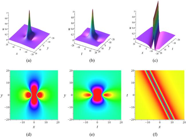
Figure 1. The first-order rogue wave u1−r with $\lambda =\tfrac{1}{2}$, α = β = 1. (a) 3D-plot of the rogue wave u1−r(x, y, 0), (b) 3D-plot of the rogue wave u1−r(0, y, t), (c) 3D-plot of the rogue wave u1−r(x, 0, t), (d) the density plot of the wave (a), (e) the density plot of the wave (b), (f) the density plot of the wave (c). |
2.2. Second-order rogue wave solution
Next, the characteristics and properties of second-order rogue wave solutions are analyzed from three different dimensions. The specific expressions of the parameters involved are listed in detail. In particular, we probe into the close relationship between the first-order rogue wave and the second-order rogue wave.
When n = 1, equation (10 ) can be expressed as11 ), the following formula can be obtained18 ) into (9 ), we have
$\begin{eqnarray}\begin{array}{rcl}f & = & {F}_{2}(X,y)+2\,{\xi }_{1}\,y\,{P}_{1}(X,y)+2\,{\xi }_{2}\,X\,{Q}_{1}(X,y)\\ & & +({\xi }_{1}^{2}+{\xi }_{2}^{2}){F}_{0}(X,y).\end{array}\end{eqnarray}$
From equation ( $\begin{eqnarray}\begin{array}{rcl}{F}_{2}(X,y) & = & {X}^{6}+({a}_{\mathrm{4,2}}\,{y}^{2}+{a}_{\mathrm{4,0}}){X}^{4}+({a}_{\mathrm{2,4}}\,{y}^{4}\\ & & +{a}_{\mathrm{2,2}}\,{y}^{2}+{a}_{\mathrm{2,0}}){X}^{2}\\ & & +{a}_{\mathrm{0,6}}\,{y}^{6}+{a}_{\mathrm{0,4}}\,{y}^{4}+{a}_{\mathrm{0,2}}\,{y}^{2}+{a}_{\mathrm{0,0}},\\ {P}_{1}(X,y) & = & {b}_{\mathrm{0,2}}\,{X}^{2}+{b}_{\mathrm{2,0}}\,{y}^{2}+{b}_{\mathrm{0,0}},\\ {Q}_{1}(X,y) & = & {c}_{\mathrm{2,0}}\,{X}^{2}+{c}_{\mathrm{0,2}}\,{y}^{2}+{c}_{\mathrm{0,0}},\\ {F}_{0}(X,y) & = & 1.\end{array}\end{eqnarray}$
Then $\begin{eqnarray}\begin{array}{rcl}f & = & {X}^{6}+({a}_{\mathrm{4,2}}\,{y}^{2}+{a}_{\mathrm{4,0}}){X}^{4}\\ & & +({a}_{\mathrm{2,4}}\,{y}^{4}+{a}_{\mathrm{2,2}}\,{y}^{2}+{a}_{\mathrm{2,0}}){X}^{2}\\ & & +{a}_{\mathrm{0,6}}\,{y}^{6}+{a}_{\mathrm{0,4}}\,{y}^{4}\\ & & +{a}_{\mathrm{0,2}}\,{y}^{2}+{a}_{\mathrm{0,0}}+2\,{\xi }_{1}\,y({b}_{\mathrm{0,2}}\,{X}^{2}+{b}_{\mathrm{2,0}}\,{y}^{2}+{b}_{\mathrm{0,0}})\\ & & +2\,{\xi }_{2}\,X({c}_{\mathrm{2,0}}\,{X}^{2}+{c}_{\mathrm{0,2}}\,{y}^{2}+{c}_{\mathrm{0,0}})+{\xi }_{1}^{2}+{\xi }_{2}^{2}.\end{array}\end{eqnarray}$
Substituting equation ( $\begin{eqnarray}\begin{array}{rcl}{a}_{\mathrm{0,0}} & = & \displaystyle \frac{\eta }{9({\lambda }^{4}-2\,\alpha \,{\lambda }^{2}+{\alpha }^{2})(-{\lambda }^{2}+\alpha )},\\ {a}_{\mathrm{0,2}} & = & \displaystyle \frac{475}{\beta (-{\lambda }^{2}+\alpha )},\\ {a}_{\mathrm{0,4}} & = & \displaystyle \frac{17(-{\lambda }^{2}+\alpha )}{{\beta }^{2}},\\ {a}_{\mathrm{0,6}} & = & \displaystyle \frac{-{\lambda }^{6}+3\,\alpha \,{\lambda }^{4}-3\,{\alpha }^{2}\,{\lambda }^{2}+{\alpha }^{3}}{{\beta }^{3}},\\ {a}_{\mathrm{2,0}} & = & -\displaystyle \frac{125}{{\lambda }^{4}-2\,\alpha \,{\lambda }^{2}+{\alpha }^{2}},{a}_{\mathrm{2,2}}=\displaystyle \frac{90}{\beta },\\ {a}_{\mathrm{2,4}} & = & \displaystyle \frac{3({\lambda }^{4}-2\,\alpha \,{\lambda }^{2}+{\alpha }^{2})}{{\beta }^{2}},\\ {a}_{\mathrm{4,0}} & = & \displaystyle \frac{25}{(-{\lambda }^{2}+\alpha )},{a}_{\mathrm{4,2}}=\displaystyle \frac{3(-{\lambda }^{2}+\alpha )}{\beta },\\ {b}_{\mathrm{0,0}} & = & \displaystyle \frac{5\,{b}_{\mathrm{0,2}}}{3(-{\lambda }^{2}+\alpha )},\\ {b}_{\mathrm{2,0}} & = & -\displaystyle \frac{(-{\lambda }^{2}+\alpha ){b}_{\mathrm{0,2}}}{3\,\beta },{c}_{\mathrm{0,0}}=-\displaystyle \frac{{c}_{\mathrm{2,0}}}{(-{\lambda }^{2}+\alpha )},\\ {c}_{\mathrm{0,2}} & = & -\displaystyle \frac{3(-{\lambda }^{2}+\alpha ){c}_{\mathrm{2,0}}}{\beta },\\ {b}_{\mathrm{0,2}} & = & {b}_{\mathrm{0,2}},{c}_{\mathrm{2,0}}={c}_{\mathrm{2,0}}.\end{array}\end{eqnarray}$
Here $\begin{eqnarray*}\begin{array}{rcl}\eta & = & -9({\lambda }^{6}-3\,\alpha \,{\lambda }^{4}+3\,{\alpha }^{2}\,{\lambda }^{2}-{\alpha }^{3}){c}_{0,2}^{2}\,{\xi }_{2}^{2}\\ & & +\beta ({\lambda }^{4}-2\,\alpha \,{\lambda }^{2}+{\alpha }^{2}){b}_{0,2}^{2}\,{\xi }_{1}^{2}\\ & & +9({\lambda }^{6}-3\,\alpha \,{\lambda }^{4}+3\,{\alpha }^{2}\,{\lambda }^{2}-{\alpha }^{3})({\xi }_{1}^{2}+{\xi }_{2}^{2})+16875.\end{array}\end{eqnarray*}$
And b0,2, c2,0, ξ1, ξ2 are arbitrary constants.When α = β = 1, $\lambda =\tfrac{1}{2}$, the second-order rogue wave solution is formed by the interaction of two first-order rogue wave solutions, as shown in figures 2(a) and (b). The main characteristics of a second order rogue wave are two high peaks and three low peaks, furthermore, the two waves are parallel to each other. In the case of y = 0, the second-order rogue u2−r has the same structure as the two solitons in figure 2(c). In particular, if we take ξ1 = ξ2 = 0, the two parallel waves have the same height.
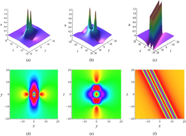
Figure 2. The second-order rogue solution u2−r with $\lambda =\tfrac{1}{2}$, α = β = 1, ξ1 = ξ2 = 0, b0,2 = c2,0 = 1. (a) 3D-plot of the rogue wave u2−r(x, y, 0), (b) 3D-plot of the rogue wave u2−r(0, y, t), (c) 3D-plot of the rogue wave u2−r(x, 0, t), (d) the density plot of the wave (a), (e) the density plot of the wave (b), (f) the density plot of the wave (c). |
2.3. Third-order rogue wave solution
According to lemma 1 , the image properties of the third-order rogue wave solution of equation (3 ) are visualized. It can be seen from the image that the rogue wave solution is mainly divided into two categories, namely, the lump wave and the line rogue wave. It is not difficult to conclude that high-order rogue waves are formed by the interaction of a finite number of first order rogue waves. In addition, a series of parameter formulas can be deduced.
When n = 2, equation (10 ) is expressed as11 ), we get
$\begin{eqnarray}\begin{array}{rcl}f & = & {F}_{3}(X,y)+2\,{\xi }_{1}\,y\,{P}_{2}(X,y)+2\,{\xi }_{2}\,X\,{Q}_{2}(X,y)\\ & & +({\xi }_{1}^{2}+{\xi }_{2}^{2}){F}_{1}(X,y).\end{array}\end{eqnarray}$
And from equation ( $\begin{eqnarray}\begin{array}{rcl}{F}_{3}(X,y) & = & {X}^{12}+({a}_{\mathrm{10,2}}\,{y}^{2}+{a}_{\mathrm{10,0}}){X}^{10}\\ & & +({a}_{\mathrm{8,4}}\,{y}^{4}+{a}_{\mathrm{8,2}}\,{y}^{2}+{a}_{\mathrm{8,0}}){X}^{8}\\ & & +\left({a}_{\mathrm{6,6}}\,{y}^{6}+{a}_{\mathrm{6,4}}\,{y}^{4}+{a}_{\mathrm{6,2}}\,{y}^{2}+{a}_{\mathrm{6,0}}\right){X}^{6}\\ & & +\left({a}_{\mathrm{4,8}}\,{y}^{8}+{a}_{\mathrm{4,6}}\,{y}^{6}+{a}_{\mathrm{4,4}}\,{y}^{4}+{a}_{\mathrm{4,2}}\,{y}^{2}\right.\\ & & \left.+{a}_{\mathrm{4,0}}\right){X}^{4}+\left({a}_{\mathrm{2,10}}\,{y}^{10}+{a}_{\mathrm{2,8}}\,{y}^{8}\right.\\ & & \left.+{a}_{\mathrm{2,6}}\,{y}^{6}+{a}_{\mathrm{2,4}}\,{y}^{4}+{a}_{\mathrm{2,2}}\,{y}^{2}+{a}_{\mathrm{2,0}}\right){X}^{2}\\ & & +{a}_{\mathrm{0,12}}\,{y}^{12}+{a}_{\mathrm{0,10}}\,{y}^{10}+{a}_{\mathrm{0,8}}\,{y}^{8}+{a}_{\mathrm{0,6}}\,{y}^{6}\\ & & +{a}_{\mathrm{0,4}}\,{y}^{4}+{a}_{\mathrm{0,2}}\,{y}^{2}+{a}_{\mathrm{0,0}},\\ {P}_{2}(X,y) & = & {b}_{\mathrm{0,6}}\,{X}^{6}+{b}_{\mathrm{2,4}}\,{X}^{4}\,{y}^{2}+{b}_{\mathrm{4,2}}\,{X}^{2}\,{y}^{4}+{b}_{\mathrm{6,0}}\,{y}^{6}\\ & & +{b}_{\mathrm{0,4}}\,{X}^{4}+{b}_{\mathrm{2,2}}\,{X}^{2}\,{y}^{2}+{b}_{\mathrm{4,0}}\,{y}^{4}\\ & & +{b}_{\mathrm{0,2}}\,{X}^{2}+{b}_{\mathrm{2,0}}\,{y}^{2}+{b}_{\mathrm{0,0}},\\ {Q}_{2}(X,y) & = & {c}_{\mathrm{6,0}}\,{X}^{6}+{c}_{\mathrm{4,2}}\,{X}^{4}\,{y}^{2}+{c}_{\mathrm{2,4}}\,{X}^{2}\,{y}^{4}+{c}_{\mathrm{0,6}}\,{y}^{6}\\ & & +{c}_{\mathrm{4,0}}\,{X}^{4}+{c}_{\mathrm{2,2}}\,{X}^{2}\,{y}^{2}+{c}_{\mathrm{0,4}}\,{y}^{4}\\ & & +{c}_{\mathrm{2,0}}\,{X}^{2}+{c}_{\mathrm{0,2}}\,{y}^{2}+{c}_{\mathrm{0,0}},\\ {F}_{1}(X,y) & = & {a}_{\mathrm{0,2}}\,{y}^{2}+{X}^{2}+{a}_{\mathrm{0,0}}.\end{array}\end{eqnarray}$
The parameter expression is as follows: $\begin{eqnarray*}\begin{array}{rcl}{a}_{\mathrm{0,0}} & = & \displaystyle \frac{9\,{\phi }_{9}\,{c}_{2,0}^{2}\,{\xi }_{2}^{2}+21609\,\beta \,{\phi }_{4}\,{b}_{0,6}^{2}\,{\xi }_{1}^{2}+17583844050208}{180075\,{\phi }_{6}({\xi }_{1}^{2}+{\xi }_{2}^{2}+1)},\\ {a}_{\mathrm{0,2}} & = & \displaystyle \frac{3\,{\phi }_{9}\,{c}_{2,0}^{2}\,{\xi }_{2}^{2}+7203\,\beta \,{\phi }_{4}\,{b}_{0,6}^{2}\,{\xi }_{1}^{2}+18061327418750}{180075\,\beta \,{\phi }_{4}({\xi }_{1}^{2}+{\xi }_{2}^{2}+1)},\\ {a}_{\mathrm{0,4}} & = & \displaystyle \frac{16391725}{3\,{\beta }^{2}\,{\phi }_{2}},\,{a}_{\mathrm{0,6}}=\displaystyle \frac{798980}{3\,{\beta }^{3}},\,{a}_{\mathrm{0,8}}=\displaystyle \frac{4335\,{\phi }_{2}}{{\beta }^{4}},\,{a}_{\mathrm{0,10}}=\displaystyle \frac{58\,{\phi }_{4}}{{\beta }^{5}},\\ {a}_{\mathrm{0,12}} & = & \displaystyle \frac{{\phi }_{6}}{{\beta }^{6}},\,{a}_{\mathrm{2,0}}=\displaystyle \frac{3\,{\phi }_{9}\,{c}_{2,0}^{2}\,{\xi }_{2}^{2}-180075\,{\phi }_{5}({\xi }_{1}^{2}+{\xi }_{2}^{2})+9591187663750}{180075\,{\phi }_{2}\,{\phi }_{3}},\\ {a}_{\mathrm{2,2}} & = & \displaystyle \frac{565950}{\beta \,{\phi }_{3}},\,{a}_{\mathrm{2,4}}=-\displaystyle \frac{14700}{{\beta }^{2}\,{\phi }_{1}},\,{a}_{\mathrm{2,6}}=\displaystyle \frac{35420\,{\phi }_{1}}{{\beta }^{3}},\,{a}_{\mathrm{2,8}}=\displaystyle \frac{570\,{\phi }_{3}}{{\beta }^{4}},\end{array}\end{eqnarray*}$
$\begin{eqnarray}\begin{array}{rcl}{a}_{\mathrm{2,10}} & = & \displaystyle \frac{6\,{\phi }_{5}}{{\beta }^{5}},\,{a}_{\mathrm{4,0}}=-\displaystyle \frac{5187875}{3\,{\phi }_{4}},\,{a}_{\mathrm{4,2}}=\displaystyle \frac{220500}{\beta \,{\phi }_{2}},\,{a}_{\mathrm{4,4}}=\displaystyle \frac{37450}{{\beta }^{2}},\,{a}_{\mathrm{4,6}}=\displaystyle \frac{1460\,{\phi }_{2}}{{\beta }^{3}},\\ {a}_{\mathrm{4,8}} & = & \displaystyle \frac{15\,{\phi }_{4}}{{\beta }^{4}},\,{a}_{\mathrm{6,0}}=\displaystyle \frac{75460}{3\,{\phi }_{3}},\,{a}_{\mathrm{6,2}}=\displaystyle \frac{18620}{\beta \,{\phi }_{1}},\,{a}_{\mathrm{6,4}}=\displaystyle \frac{1540\,{\phi }_{1}}{{\beta }^{2}},\,{a}_{\mathrm{6,6}}=\displaystyle \frac{20\,{\phi }_{3}}{{\beta }^{3}},\\ {a}_{\mathrm{8,0}} & = & \displaystyle \frac{735}{{\phi }_{2}},\,{a}_{\mathrm{8,2}}=\displaystyle \frac{690}{\beta },\,{a}_{\mathrm{8,4}}=\displaystyle \frac{15\,{\phi }_{2}}{{\beta }^{2}},\,{a}_{\mathrm{10,0}}=\displaystyle \frac{98}{{\phi }_{1}},\,{a}_{\mathrm{10,2}}=\displaystyle \frac{6\,{\phi }_{1}}{\beta },\,{b}_{\mathrm{0,0}}=\displaystyle \frac{3773\,{b}_{\mathrm{0,6}}}{3\,{\phi }_{3}},\\ {b}_{\mathrm{0,2}} & = & -\displaystyle \frac{133\,{b}_{\mathrm{0,6}}}{{\phi }_{2}},\,{b}_{\mathrm{0,4}}=\displaystyle \frac{21\,{b}_{\mathrm{0,6}}}{{\phi }_{1}},\,{b}_{\mathrm{2,0}}=-\displaystyle \frac{49\,{b}_{\mathrm{0,6}}}{\beta \,{\phi }_{1}},\,{b}_{\mathrm{2,2}}=-\displaystyle \frac{38\,{b}_{\mathrm{0,6}}}{\beta },\\ {b}_{\mathrm{2,4}} & = & -\displaystyle \frac{{b}_{\mathrm{0,6}}\,{\phi }_{1}}{\beta },\,{b}_{\mathrm{4,0}}=-\displaystyle \frac{7\,{b}_{\mathrm{0,6}}\,{\phi }_{1}}{5\,{\beta }^{2}},\,{b}_{\mathrm{4,2}}=-\displaystyle \frac{9\,{b}_{\mathrm{0,6}}\,{\phi }_{2}}{5\,{\beta }^{2}},\,{b}_{\mathrm{6,0}}=\displaystyle \frac{{b}_{\mathrm{0,6}}\,{\phi }_{2}\,{\phi }_{1}}{5\,{\beta }^{2}},\\ {c}_{\mathrm{0,0}} & = & -\displaystyle \frac{49\,{c}_{\mathrm{2,0}}}{3\,{\phi }_{1}},\,{c}_{\mathrm{0,2}}=-\displaystyle \frac{107\,{c}_{\mathrm{2,0}}\,{\phi }_{1}}{49\,\beta },\,{c}_{\mathrm{0,4}}=-\displaystyle \frac{9\,{c}_{\mathrm{2,0}}\,{\phi }_{3}}{49\,{\beta }^{2}},\,{c}_{\mathrm{0,6}}=-\displaystyle \frac{{c}_{\mathrm{2,0}}\,{\phi }_{2}^{2}\,{\phi }_{1}}{49\,{\beta }^{3}},\\ {c}_{\mathrm{2,2}} & = & \displaystyle \frac{46\,{c}_{\mathrm{2,0}}\,{\phi }_{1}^{2}}{49\,\beta },\,{c}_{\mathrm{2,4}}=\displaystyle \frac{{c}_{\mathrm{2,0}}\,{\phi }_{2}^{2}}{49\,{\beta }^{2}},\,{c}_{\mathrm{4,0}}=\displaystyle \frac{13\,{c}_{\mathrm{2,0}}\,{\phi }_{1}}{245},\,{c}_{\mathrm{4,2}}=\displaystyle \frac{9\,{c}_{\mathrm{2,0}}\,{\phi }_{2}\,{\phi }_{1}}{245\,\beta },\\ {c}_{\mathrm{6,0}} & = & -\displaystyle \frac{{c}_{\mathrm{2,0}}\,{\phi }_{2}}{245},\,{b}_{\mathrm{0,6}}={b}_{\mathrm{0,6}},{c}_{\mathrm{2,0}}={c}_{\mathrm{2,0}}.\end{array}\end{eqnarray}$
Here $\begin{eqnarray*}{\phi }_{n}={(-{\lambda }^{2}+\alpha )}^{n},\end{eqnarray*}$
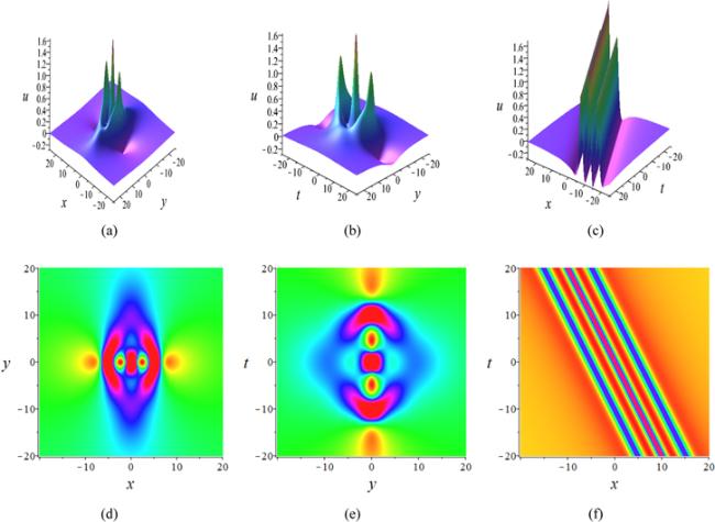
where n is a positive integer, and b0,6, c2,0, ξ1, ξ2 are arbitrary constants.Different from the second-order rogue wave, the third-order rogue wave is composed of three first-order rogue waves with different amplitudes (see figures 3(a) and (b)). It is not difficult to see that the amplitude of the waves in the middle is higher than that on both sides and that the waves on both sides have the same amplitude. Moreover, when y = 0 and ξ1 = ξ2 = 0, the third-order rogue wave has the structure of three solitons in the plane (x, t) (see figure 3(c)).
Figure 3. The third-order rogue solution u3−r with $\lambda =\tfrac{1}{2}$, α = β = 1, ξ1 = ξ2 = 0, b0,6 = c2,0 = 1. (a) 3D-plot of the rogue wave u3−r(x, y, 0), (b) 3D-plot of the rogue wave u3−r(0, y, t), (c) 3D-plot of the rogue wave u3−r(x, 0, t), (d) the density plot of the wave (a), (e) the density plot of the wave (b), (f) the density plot of the wave (c). |
3. Conclusions
In this paper, we mainly study the multiple-order rogue wave solutions of the (2+1)-dimensional Boussinesq type equation. The reduced form of equation (3 ) can be obtained by the variable substitution X = x + λt, and it can be transformed into a bilinear form under the logarithmic transformation $u=2{(\mathrm{ln}f)}_{{XX}}$. Based on the reduced bilinear equation, first-order, second-order and third-order rogue wave solutions can be obtained by the symbolic computation approach (see figures 1–3). Through the above analysis, it can be seen that the maximum value of each rogue wave solution is located on the line y = 0. In particular, the maximum and minimum points of the first-order rogue wave can be determined by the extremum discriminant method of multi-variable differential. In addition, in planes (x, y) and (y, t), the multiple-order rogue wave solutions exhibit the lump-type solutions. However, in-plane (x, t), the multiple-order rogue waves are in the form of multi-solitons, that is, line rogue waves. The results of this article may help explain the nonlinear phenomena in fluid mechanics.