


1. Introduction
NLSEs are the stem of various studies in the physics of nonlinear optics. These equations have the property that, in the presence of Kerr nonlinearity, they are integrable when the real and imaginary parts are linearly dependent. The PNLSE was remarkably analyzed in the literature. It describes the pulse propagation that results from self-steepening, self-phase modulation and third-order dispersion interaction. Also, it is used for investigating an ultra-short optical pulse propagating along the nonlinear fibers with the Raman effect and self-steepening. Single-mode propagation of ultrashort optical pulse is governed by a generalized NLSE. An extended version of a NLSE, including polarization effects, high-order dispersion, Kerr and Raman nonlinearities, self-steepening effects, as well as wavelength-dependent mode coupling and nonlinear coefficients, was studied in [1]. In [2], the inverse scattering transform with one parameter was used to inspect the breather-like four-parameter soliton solutions. By using the extended sinh-Gordon expansion method, the space-time fractional PNLSE equation was considered in [3]. In [4], the extension of the rational sine-cosine method and rational sinh-cosh method was employed to construct the exact traveling wave solutions of PNLSE. In The two variables (G′/G, 1/G)-expansion method, to obtain abundant closed-form wave solutions to the PNLSE, was implemented [5]. Dark and singular solitons for the resonance PNLSE, with beta derivative, were investigated in [6]. The conformable fractional derivative was used for constructing exact solitary wave solutions to the fractional PNLSE with quantic nonlinearity. Further, the effects of nonlinearity on the ultrashort optical solitons pulse propagation in non-Kerr media were investigated in [7]. In [8], complex solitons in the PNLSE model, with the help of an analytical method, were obtained. By using the modified mapping method and the extended mapping method, some exact solutions of the PNLSE were obtained in [9, 10]. In [11], the PNLSE has been investigated using the sub-equation expansion method. Further relevant works were carried out in [12–15]. In [16], the problems of the existence of quasi-periodic and almost-periodic solutions and diffusion for NLSEs with a random potential were analyzed. The chiral NLSE, with perturbation term and a coefficient of Bohm potential, was considered in [17, 18]. The variational iteration method for obtaining bright and dark optical solitons for (2+1)-dimensional NLSE, that appear in the anomalous dispersion regimes has been considered in [19]. An analytic description of NLSE breather propagation in optical fibers, with strong temporal and spatial localization, was investigated in [20]. The Kundu–Mukherjee–Naskar equation was studied, with the aid of the extended trial function method to recover optical soliton solutions in (2+1)–dimensions, in [21]. In [22], a new coupled NLSE was proposed where it is proved that it is completely integrable. The improved ${\tan }(\varphi (\xi ))$ expansion method was employed to find the solutions of the PNLSE [23]. The direct algebraic method and the first integral method were used in [24] and [25] respectively for finding exact solutions of the PNLSE. Here, the extended unified method is used to find similariton solutions of the PNLSE. Together with introducing complex amplitude transformations [26–32]. Relevant works were also carried out in [33–39]
The outlines of this paper are as in what it follows. In section 2 , mathematical formulation and outlines of the extended unified method are presented. Section 3 is devoted to polynomial solutions, while rational solutions are found in section 4 . Modulation instability is studied in section 4 . Section 5 is devoted to conclusions.
2. Mathematical formulation
The study of the propagation of optical pulses in optical fibers, by taking into account third order dispersion, self-steepening of pulse and self-phase modulation is of great interest. These effects are impeded in the PNLSE proposed in [31, 32]. This equation reads,1 ) α , β and γ are the coefficients of the third order dispersion, self-steepening and self-phase modulation respectively. We use a transformation that depicts the waves produced by soliton-periodic wave collision into (1 ),
$\begin{eqnarray}\begin{array}{l}{\rm{i}}\,{w}_{t}+{h}_{1}{w}_{{xx}}+{h}_{2}| w{| }^{2}w\\ \quad -\,{\rm{i}}(\alpha \,{w}_{{xxx}}+\beta {\left(| w{| }^{2}w\right)}_{x}\\ \quad +\,\gamma {\left(| w{| }^{2}\right)}_{x}w)=0,\end{array}\end{eqnarray}$
where w = w(x, t) is a complex function, h1 is the dispersion coefficient, h2 is the coefficient of Kerr nonlinearity, and stands for self-focusing or self-defocusing according to when h2 > 0 or h2 < 0 respectively. In ( $\begin{eqnarray}\begin{array}{rcl}w(x,t) & = & (u(x,t)+{\rm{i}}v(x,t)){{\rm{e}}}^{{\rm{i}}({kx}-{\displaystyle \int }_{0}^{t}\omega (s){\rm{d}}{s})},\\ {w}^{* }(x,t) & = & (u(x,t)-{\rm{i}}v(x,t)){{\rm{e}}}^{-({kx}-{\displaystyle \int }_{0}^{t}\omega (s){\rm{d}}{s}))},\end{array}\end{eqnarray}$
and we get, $\begin{eqnarray}\begin{array}{l}-({h}_{1}{k}^{2}+{k}^{3}\alpha )u+({h}_{2}+k\beta ){u}^{3}+({h}_{2}\\ \quad +\,k\beta ){{uv}}^{2}+u\omega (t)-{v}_{t}\\ \quad +\,(-2{h}_{1}k-3{k}^{2}\alpha +\beta {u}^{2}+3\beta {v}^{2}){v}_{x}+2\gamma {v}^{2}){v}_{x}\\ \quad +\,2(\beta +\gamma ){{uvu}}_{x}+({h}_{1}+3k\alpha ){u}_{{xx}}+\alpha {v}_{{xxx}}=0,\end{array}\end{eqnarray}$
$\begin{eqnarray*}\begin{array}{l}v\omega (t)+{u}_{t}+{u}_{x}(2{h}_{1}k+3{k}^{2}\alpha -3\beta {u}^{2}-2\gamma {u}^{2}-\beta {v}^{2})\\ \quad -\,({h}_{1}{k}^{2}+{k}^{3}\alpha )v+({h}_{2}+k\beta ){u}^{2}v-2(\beta +\gamma ){{uvv}}_{x}\\ \quad +\,({h}_{2}+k\beta ){v}^{3}+({h}_{1}+3k\alpha ){v}_{{xx}}-\alpha {u}_{{xxx}}=0.\end{array}\end{eqnarray*}$
To find similariton solutions of (1 ), we introduce the similarity transformations u(x, t) = U(z, t), v(x, t) = V(z, t), z = μ(t) x, t: = t and (3 ) becomes,
$\begin{eqnarray}\begin{array}{l}-({h}_{1}{k}^{2}+{k}^{3}\alpha )U+({h}_{2}+k\beta ){U}^{3}\\ \quad +\,({h}_{2}+k\beta ){{UV}}^{2}+U\omega (t)-{v}_{t}\\ \quad +\,\mu (t)(-2{h}_{1}k-3{k}^{2}\alpha +\beta {U}^{2}\\ \quad +\,3\beta {V}^{2})+2\gamma {V}^{2}){V}_{z}\\ \quad +\,2\mu (t)(\beta +\gamma ){{UVU}}_{z}+\mu {\left(t\right)}^{2}({h}_{1}\\ \quad +\,3k\alpha ){U}_{{zz}}+\alpha \mu {\left(t\right)}^{3}{V}_{{zzz}}==0,\end{array}\end{eqnarray}$
$\begin{eqnarray*}\begin{array}{l}V\omega (t)+{U}_{t}+\mu (t){U}_{z}(2{h}_{1}k+3{k}^{2}\alpha \\ \quad -\,3\beta {U}^{2}-2\gamma {U}^{2}-\beta {V}^{2})\\ \quad -\,({h}_{1}{k}^{2}+{k}^{3}\alpha )V+({h}_{2}+k\beta ){U}^{2}V\\ \quad -\,2\mu (t)(\beta +\gamma ){{UVV}}_{z}\\ \quad +\,({h}_{2}+k\beta ){V}^{3}+\mu {\left(t\right)}^{2}({h}_{1}+3k\alpha ){V}_{{zz}}\\ \quad -\,\alpha \mu {\left(t\right)}^{3}{U}_{{zzz}}=0.\end{array}\end{eqnarray*}$
To find the exact solutions of (4 ), we use the extended unified method which is outlined in what follows.
2.1. Extended unified method
Here, we present the outlines of the extended unified method. This method asserts that solutions of a nonlinear evolution equation are expressed in the polynomial or rational forms, in an auxiliary function that satisfies an appropriate auxiliary equation.
2.1.1. Polynomial solutions
The polynomial solution of the equation (4 ) of degree n in an auxiliary function, namely g(z, t), which satisfies an auxiliary equation, is,
$\begin{eqnarray}\begin{array}{l}U(z)=\sum _{j=0}^{n}{a}_{j}(t)g{\left(z,t\right)}^{j},{\left(g{\left(z,t\right)}_{z}\right)}^{p}\\ \,=\,\sum _{j=0}^{{kp}}{c}_{j}g{\left(z,t\right)}^{j},\\ \,{\left(g{\left(z,t\right)}_{t}\right)}^{p}=\sigma (t)\sum _{j=0}^{{kp}}{c}_{j}g{\left(z,t\right)}^{j}\ p=1,2.\end{array}\end{eqnarray}$
In (5 ) we mention that $g{\left(z,t\right)}_{{zt}}=g{\left(z,t\right)}_{{tz}}$, and $g(z,t)=G(z+{\int }_{0}^{t}\sigma (s){\rm{d}}{s}).$ First, we consider the case when p = 1. By this method, the existence of a solution requires two conditions to hold, namely the balance and the consistency conditions respectively. The first condition results from balancing the higher order derivative and nonlinear terms in (4 ). In the present case, this condition reads n = k − 1. By substituting (5 ) into (4 ) and by setting the coefficients of $g{\left(z,t\right)}^{i},i=0,1,2,\ldots ,$ equal to zero, we get a set of nonlinear algebraic equations. The consistency condition depends on:
It is worth mentioning that the extended unified method is considered as an alternative to the use of Lie symmetries of PDEs. We think that the present method prevails the technique of Lie symmetries as it is of low time cost in symbolic computation, while a long hierarchy of steps is needed in the second method.
| i | (i) the number of equations obtained in the later step, say n2. |
| ii | (ii) the number of the arbitrary parameters ai(t), ci in ( |
2.1.2. The rational function solutions
The rational function solution of (1 ) or (2 ) is taken,
$\begin{eqnarray}\begin{array}{rcl}U(z) & = & \displaystyle \frac{{\sum }_{j=0}^{n}{a}_{j}(t)g{\left(z\right)}^{j})}{{\sum }_{j=0}^{n}{s}_{j}g{\left(z\right)}^{j}},\\ {\left(g{\left(z,t\right)}_{z}\right)}^{p} & = & \sum _{j=0}^{{kp}}{c}_{j}g{\left(z,t\right)}^{j},\\ {\left(g{\left(z,t\right)}_{t}\right)}^{p} & = & \sigma (t)\sum _{j=0}^{{kp}}{c}_{j}g{\left(z,t\right)}^{j}\ p=1,2.\end{array}\end{eqnarray}$
The balance and the consistency conditions in the case of rational function solution are treated in the same way as in section 2.1. For details see [19].
The steps of computations are carried out in what follows [19]:
Step 1. Implementing (5 ) or (6 ) into (4 ), the results give rise to a set of nonlinear algebraic equations.
Step 2. Solving the auxiliary equations in (5 ) or in (6 ) to get the explicit form for g(z, t).
Step 3. Finding the exact formal solution which is given by the equations (5 ) or (6 ).
Step 4. Check that the solution obtained satisfies (4 ).
3. Polynomial solutions of (4)
Here, we consider (5 ), by bearing in mind that n = k − 1.
3.1. Case when p = 1 and k = 2
In this case, we write,
$\begin{eqnarray}\begin{array}{rcl}U(z,t) & = & {a}_{1}(t)g(z,t)+{a}_{0}(t),\\ V(z,t) & = & {b}_{1}(t)g(z,t)+{b}_{0}(t),\,\\ g{\left(z,t\right)}_{z} & = & {c}_{2}g{\left(z,t\right)}^{2}+{c}_{1}g(z,t)+{c}_{0},\\ g{\left(z,t\right)}_{t} & = & \sigma (t)({c}_{2}g{\left(z,t\right)}^{2}+{c}_{1}g(z,t)+{c}_{0}).\end{array}\end{eqnarray}$
In (7 ), for linearly dependent functions U and V, we take b0(t) = a0(t)b1(t)/a1(t). When substituting from (7 ) into (4 ) and by setting the coefficients of $g{\left(z,t\right)}^{j},j\,=\,0,1,\ldots $ equal to zero,we get,
$\begin{eqnarray}\begin{array}{rcl}{b}_{1}(t) & = & \displaystyle \frac{\sqrt{(3\beta +2\gamma ){a}_{1}{\left(t\right)}^{2}+6{c}_{2}^{2}\alpha \mu {\left(t\right)}^{2}}}{\sqrt{-(3\beta +2\gamma )}},3\beta \\ & & +2\gamma \lt 0,\,{a}_{0}(t)=\displaystyle \frac{{c}_{1}}{2{c}_{2}}{a}_{1}(t),\\ {a}_{1}(t) & = & \displaystyle \frac{\sqrt{2}\sqrt{(3\beta +2\gamma ){A}_{0}+3{c}_{2}^{2}\alpha \mu {\left(t\right)}^{2}}}{\sqrt{-(3\beta +2\gamma )}},\\ \sigma (t) & = & -\displaystyle \frac{1}{2}\mu (t)(2k(2{h}_{1}+3k\alpha )+{k}_{0}^{2}\alpha \mu {\left(t\right)}^{2})\\ & & +{k}_{0}^{2}\alpha \mu {\left(t\right)}^{2}),\,\omega (t)={k}^{2}({h}_{1}+k\alpha )\\ & & +\displaystyle \frac{1}{2}{k}_{0}^{2}({h}_{1}+3k\alpha )\mu {\left(t\right)}^{2},\\ {h}_{2} & = & \displaystyle \frac{3{h}_{1}\beta +6k\alpha \beta +2{h}_{1}\gamma +6k\alpha \gamma }{3\alpha }.\end{array}\end{eqnarray}$
The auxiliary equation solves to,
$\begin{eqnarray}\begin{array}{rcl}g(z,t) & = & \displaystyle \frac{1}{2{c}_{2}}(-{c}_{1}-{k}_{0}\tanh [\displaystyle \frac{{k}_{0}}{2}(z-\displaystyle \frac{1}{2}{\displaystyle \int }_{0}^{t}\mu (s)\\ & & \times \left(2k(2{h}_{1}+3\alpha k)+\alpha {k}_{0}^{2}\mu {\left(s\right)}^{2}\right){\rm{d}}{s})),\\ {k}_{0} & = & \sqrt{{c}_{1}^{2}-4{c}_{2}{c}_{0}}.\end{array}\end{eqnarray}$
Finally, the solutions are,
$\begin{eqnarray}\begin{array}{rcl}U(z,t) & = & -\displaystyle \frac{\sqrt{2}}{\sqrt{{c}_{2}}\sqrt{-2(3\beta +2\gamma )\sqrt{{A}_{0}}}}V(z,t)\\ & & \times \sqrt{3{A}_{0}\beta +2{A}_{0}\gamma +3{c}_{2}^{2}\alpha \mu {\left(t\right)}^{2}},\\ V(z,t) & = & -\displaystyle \frac{{k}_{0}\sqrt{{A}_{0}}}{\sqrt{2}{c}_{2}}\tanh (\displaystyle \frac{{k}_{0}}{2}(z-\displaystyle \frac{1}{2}{\displaystyle \int }_{0}^{t}\mu (s)\\ & & \times \left(2k(2{h}_{1}+3\alpha k)+\alpha {k}_{0}^{2}\mu {\left(s\right)}^{2}\right){ds})),\end{array}\end{eqnarray}$
where μ(t) is arbitrary.The results in (10) are used to calculate ∣w(x, t)∣ and Re w(x, t) which are,10 ).
$\begin{eqnarray}| \begin{array}{rcl}w(x,t)| & = & \sqrt{u{\left(x,t\right)}^{2}+v{\left(x,t\right)}^{2}}\\ & = & \sqrt{U{\left(z,t\right)}^{2}+V{\left(z,t\right)}^{2}}\\ {\rm{Re}}\,{w}(x,t) & = & u(x,t)\cos ({kx}-{\displaystyle \int }_{0}^{t}\omega (s){ds})\\ & & -v(x,t)\sin ({kx}-{\displaystyle \int }_{0}^{t}\omega (s){ds})\\ & = & U(z,t)\cos ({kx}-{\displaystyle \int }_{0}^{t}\omega (s){ds})\\ & & -V(z,t)\sin ({kx}-{\displaystyle \int }_{0}^{t}\omega (s){ds}),\\ z & = & \mu (t)x,\end{array}\end{eqnarray}$
where U(z, t) and V(z, t) are given in (By using (11 ) and (10 ) are used to calculate ∣w(x, t)∣ and Re w(x, t) and they are evaluated numerically. The results are shown in figures 1(i)–(iv).
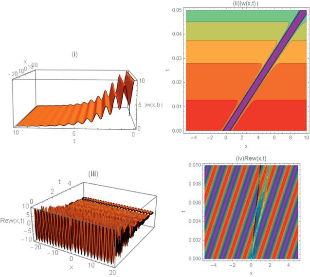
When β = −1.5, γ = 0.8, k = 4, h1 = 0.9, c2 = 3.7, α = 1.9, k0 = 2.5, A0 = 1.5,
$\mu (t)={\rm{{\rm{sech}} }}(0.6t)(3+\cos (8t))$. Figure 1(i) shows a cascade of solitons towards steepening near t = 0. Also, figure 1(ii) shows self steepening which progress to shock solitons near t = 0. Figure 1(ii) shows, also, a cascade of solitons with quasi-self-modulation in time. Figure 1(iv) shows self-phase modulation with steepening near the origin.
3.2. When p = 2 and k = 2
Here, we consider (7 ) with the auxiliary equation,
$\begin{eqnarray}\begin{array}{rcl}g{\left(z,t\right)}_{z} & = & g(z,t)\sqrt{{c}_{2}g{\left(z,t\right)}^{2}+{c}_{1}g(z,t)+{c}_{0}},\\ g{\left(z,t\right)}_{z} & = & \sigma (t)g(z,t)\sqrt{{c}_{2}g{\left(z,t\right)}^{2}+{c}_{1}g(z,t)+{c}_{0}}.\end{array}\end{eqnarray}$
By inserting (7 ) and (15 ) into (4 ), we have,
$\begin{eqnarray}\begin{array}{rcl}{b}_{1}(t) & = & \displaystyle \frac{\sqrt{\alpha (({h}_{2}+k\beta ){a}_{1}{\left(t\right)}^{2}+2{c}_{2}({h}_{1}+3k\alpha )\mu {\left(t\right)}^{2})}}{\sqrt{-(3\beta +2\gamma )({h}_{1}+k\alpha )}},\\ \,3\beta +2\gamma \lt 0,{a}_{1}(t) & = & \displaystyle \frac{4{c}_{2}{a}_{0}(t)}{{c}_{1}},\,{c}_{0}=\displaystyle \frac{{c}_{1}^{2}}{4{c}_{2}},\\ {a}_{0}(t) & = & \displaystyle \frac{\sqrt{\alpha ({A}_{0}+{c}_{1}^{2}({h}_{1}+3k\alpha )\mu {\left(t\right)}^{2})}}{\sqrt{-(3\beta +2\gamma )({h}_{1}+k\alpha )}},\\ {h}_{2} & = & 2k(\beta +\gamma )+\displaystyle \frac{{h}_{1}(3\beta +2\gamma )}{3\alpha },\\ \sigma (t) & = & -k(2{h}_{1}+3k\alpha )\mu (t)-\displaystyle \frac{{c}_{1}^{2}\alpha \mu {\left(t\right)}^{3}}{8{c}_{2}},\\ \omega (t) & = & {k}^{2}({h}_{1}+k\alpha )+\displaystyle \frac{{c}_{1}^{2}({h}_{1}+3k\alpha )\mu {\left(t\right)}^{2}}{8{c}_{2}},\\ {b}_{0}(t) & = & \displaystyle \frac{{a}_{0}(t){b}_{1}(t)}{{a}_{1}(t)}.\end{array}\end{eqnarray}$
The auxiliary function is,
$\begin{eqnarray}\begin{array}{l}g(z,t)=-\,\displaystyle \frac{{c}_{1}{{\rm{e}}}^{\tfrac{{c}_{1}}{\sqrt{{c}_{2}}}(\tfrac{z}{2}-{\displaystyle \int }_{0}^{t}\left(\tfrac{\alpha {c}_{1}^{2}\mu {\left(s\right)}^{3}}{8{\rm{c}}2}+k\mu (s)\left(2{h}_{1}+3\alpha k\right)\right){\rm{d}}{s})}}{-1+2{c}_{2}{{\rm{e}}}^{\tfrac{{c}_{1}}{\sqrt{{c}_{2}}}(\tfrac{z}{2}-{\displaystyle \int }_{0}^{t}\left(\tfrac{\alpha {c}_{1}^{2}\mu {\left(s\right)}^{3}}{8{\rm{c}}2}+k\mu (s)\left(2{h}_{1}+3\alpha k\right)\right){\rm{d}}{s})}}.\end{array}\end{eqnarray}$
Finally, the solutions are,
$\begin{eqnarray}\begin{array}{l}U(z,t)=-\displaystyle \frac{{P}_{1}}{Q},\quad {P}_{1}=\sqrt{3/2}\sqrt{{A}_{0}+{c}_{1}^{2}({h}_{1}+3k\alpha )\mu {\left(t\right)}^{2}}(1+2{c}_{2}\\ \,\times \,{{\rm{e}}}^{\tfrac{{c}_{1}}{\sqrt{{c}_{2}}}(\displaystyle \frac{z}{2}-{\displaystyle \int }_{0}^{t}\left(\displaystyle \frac{\alpha {c}_{1}^{2}\mu {\left(s\right)}^{3}}{8{\rm{c}}2}+k\mu (s)\left(2{h}_{1}+3\alpha k\right)\right){\rm{d}}{s})}),\\ \quad Q=2\sqrt{{c}_{2}}\sqrt{-({h}_{1}+3k\alpha )(3\beta +2\gamma )\alpha }(-1+2{c}_{2}\\ \,\times \,{{\rm{e}}}^{\tfrac{{c}_{1}}{\sqrt{{c}_{2}}}(\displaystyle \frac{z}{2}-{\displaystyle \int }_{0}^{t}\left(\displaystyle \frac{\alpha {c}_{1}^{2}\mu {\left(s\right)}^{3}}{8{\rm{c}}2}+k\mu (s)\left(2{h}_{1}+3\alpha k\right)\right){\rm{d}}{s})}),\\ \quad V(z,t)=\displaystyle \frac{U(z,t)}{\sqrt{{c}_{2}}\sqrt{{A}_{0}+{c}_{1}^{2}({h}_{1}+3k\alpha )\mu {\left(t\right)}^{2}}}.\end{array}\end{eqnarray}$
The equations (10 ) and (15 )are used to calculate ∣w(x, t)∣ and Re w(x, t) and they are evaluated numerically. The results are shown in figures 2(i)–(iv).
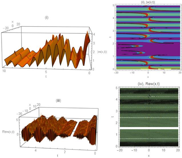
When β = −1.5, γ = 0.8, k = 4.5, h1 = 0.9, c2 = 3.7, α = 1.9, c1 = 2.5, A0 = −1.5, $\mu (t)={\rm{{\rm{sech}} }}(0.06t)(3\sin (7t)+\cos (8t))$. Figure 2(i) shows oscillatory waves with cusps and self-steepening near t = 0. Also, figure 2 (ii) shows, also, self- steepening. Figure 2(iii) shows a rhombus pattern (diamond) with self-phase modulation solitons in time. Figure 2(iv) shows, also, self-phase modulation.
3.3. When p = 1 and k = 3
The solutions are written,
$\begin{eqnarray}\begin{array}{rcl}U(z,t) & = & {a}_{2}(t)g{\left(z,t\right)}^{2}+{a}_{1}(t)g(z,t)+{a}_{0}(t),\\ V(z,t) & = & {b}_{2}(t)g{\left(z,t\right)}^{2}+{b}_{1}(t)g(z,t)+{b}_{0}(t),\\ g{\left(z,t\right)}_{z} & = & {c}_{3}g{\left(z,t\right)}^{3}+{c}_{2}g{\left(z,t\right)}^{2}+{c}_{1}g(z,t)+{c}_{0},\\ g{\left(z,t\right)}_{t} & = & \sigma (t)({c}_{3}g{\left(z,t\right)}^{3}+{c}_{2}g{\left(z,t\right)}^{2}+{c}_{1}g(z,t)+{c}_{0}).\end{array}\end{eqnarray}$
For linearly dependent solutions, we take b0(t) =a0(t)b1(t)/a1(t), and b2(t) = a2(t)b1(t)/a1(t). By inserting (12 ) into (4 ), we have,
$\begin{eqnarray}\begin{array}{rcl}{b}_{1}(t) & = & \displaystyle \frac{{a}_{1}(t)\sqrt{(3\beta +2\gamma ){a}_{2}{\left(t\right)}^{2}+24{c}_{3}^{2}\alpha \mu {\left(t\right)}^{2}}}{{a}_{2}(t)\sqrt{-(3\beta +2\gamma )}},\\ {a}_{1}(t) & = & \displaystyle \frac{2{c}_{2}{a}_{2}(t)}{3{c}_{3}},3\beta +2\gamma \lt 0,\\ {h}_{2} & = & 2k(\beta +\gamma ),\,{c}_{0}=\displaystyle \frac{-2{c}_{2}^{3}+9{c}_{1}{c}_{2}{c}_{3}}{27{c}_{3}^{2}},\\ \sigma (t) & = & -k(2{h}_{1}+3k\alpha \mu (t)\\ & & -(4{\left({c}_{2}^{2}-3{c}_{1}{c}_{3}\right)}^{2}\displaystyle \frac{\alpha (2{h}_{1}+27k\alpha )\mu {\left(t\right)}^{3}}{9{h}_{1}{c}_{3}^{2}},\,\omega (t)=\displaystyle \frac{P}{Q},\\ P & = & (-6{c}_{3}^{4}{{Mh}}_{1}^{2}{k}^{2}{\alpha }^{3/2}({h}_{1}+k\alpha ))\\ & & \times \sqrt{-(3\beta +2\gamma )}\mu {\left(t\right)}^{3}-8{c}_{3}^{2}{M}^{3}k{\alpha }^{5/2}(2{h}_{1}^{2}+3{h}_{1}k\alpha +3{k}^{2}{\alpha }^{2})\\ & & \times \sqrt{-(3\beta +2\gamma )}\mu {\left(t\right)}^{5}-64{M}^{5}k\setminus {\alpha }^{9/2}\\ & & \times \sqrt{-(3\beta +2\gamma )}\mu {\left(t\right)}^{7}\\ & & -3{c}_{3}^{3}{h}_{1}^{2}\sqrt{\displaystyle \frac{{c}_{3}^{4}{h}_{1}^{2}\alpha \mu {\left(t\right)}^{2}}{({c}_{3}^{2}{h}_{1}^{2}+4{M}^{2}{\alpha }^{2}\mu {\left(t\right)}^{2})}}\\ & & \times \sqrt{-(3\beta +2\gamma )({c}_{3}^{2}{h}_{1}^{2}+4{M}^{2}{\alpha }^{2}\mu {\left(t\right)}^{2})}{\mu }^{{\prime} }(t)),\\ Q & = & (-6{c}_{3}^{2}M{\alpha }^{3/2})\sqrt{-(3\beta +2\gamma )}\mu {\left(t\right)}^{3}\\ & & \times ({c}_{3}^{2}{h}_{1}^{2}+4{M}^{2}{\alpha }^{2}\mu {\left(t\right)}^{2}),\\ M & = & {c}_{2}^{2}-3{c}_{1}{c}_{3},{a}_{2}(t)=(\sqrt{-(3\beta +2\gamma )})({c}_{3}^{2}{h}_{1}^{2}+4{M}^{2}{\alpha }^{2}\mu {\left(t\right)}^{2},\\ {a}_{0}(t) & = & -\displaystyle \frac{2\sqrt{2/3}}{(3{c}_{3}^{5}{h}_{1}^{2}{\left(-(3\beta +2\gamma )\right)}^{3/2}}M{\alpha }^{1/2}\\ & & \times \sqrt{\displaystyle \frac{{c}_{3}^{4}{h}_{1}^{2}\alpha \mu {\left(t\right)}^{2}}{({c}_{3}^{2}{h}_{1}^{2}+4{M}^{2}{\alpha }^{2}\mu {\left(t\right)}^{2})}}\\ & & \times (3{c}_{3}^{2}{{Mh}}_{1}(3\beta +2\gamma )\mu (t)+M\sqrt{-(3\beta +2\gamma )}\\ & & \times \sqrt{\displaystyle \frac{{c}_{3}^{4}{h}_{1}^{2}\alpha \mu {\left(t\right)}^{2}}{({c}_{3}^{2}{h}_{1}^{2}+4{M}^{2}{\alpha }^{2}\mu {\left(t\right)}^{2})}}\\ & & \times \sqrt{-(3\beta +2\gamma )}({c}_{3}^{2}{h}_{1}^{2}+4{M}^{2}{\alpha }^{2}\mu {\left(t\right)}^{2}.\end{array}\end{eqnarray}$
The final solutions are,
$\begin{eqnarray}\begin{array}{rcl}U(z,t) & = & \displaystyle \frac{4{A}_{0}{M}^{2}{\alpha }^{3/2}\mu {\left(t\right)}^{2}}{{c}_{3}({A}_{0}+{{\rm{e}}}^{\tfrac{2M}{3c}(z-B(t))})\sqrt{-(3\beta +2\gamma )}\sqrt{{c}_{3}^{2}{h}_{1}^{2}+4{M}^{2}{\alpha }^{2}\mu {\left(t\right)}^{2}}},\\ V(z,t) & = & \displaystyle \frac{2{A}_{0}\sqrt{2/3}{{Mh}}_{1}{\alpha }^{1/2}(-(3\beta +2\gamma ))\mu (t)({{ch}}_{1}^{2}+4{M}^{2}{\alpha }^{2}\mu {\left(t\right)}^{2})}{({A}_{0}+{{\rm{e}}}^{\tfrac{2M}{3c}(z-B(t))})\sqrt{-(3\beta +2\gamma )}\sqrt{{c}_{3}^{2}{h}_{1}^{2}+4{M}^{2}{\alpha }^{2}\mu {\left(t\right)}^{2}}}\\ u(x,t) & = & U(z,t),\quad v(x,t)=V(z,t),\,z=\mu (t)x,.\\ B(t) & = & {\displaystyle \int }_{0}^{t}\displaystyle \frac{4\alpha \left({c}_{2}^{2}-3{c}_{1}{c}_{3}\right){}^{2}\mu {\left(t\right)}^{3}\left(2{h}_{1}+27\alpha k\right)}{9{c}_{3}^{2}{h}_{1}}+k\mu (t)\left(2{h}_{1}+3\alpha k\right).\end{array}\end{eqnarray}$
The equations (10 ) and (18 ) are used to calculate ∣w(x, t)∣ and Re w(x, t) and they are evaluated numerically. The results are shown in figures 3(i)–(iv).
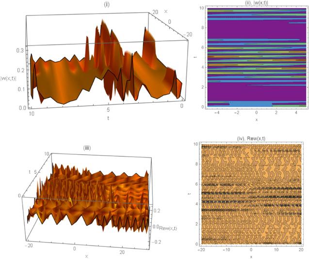
When β = −1.5, γ = 0.8, k0:=0.5, k = 4, h1 = 0.9, c2 = 1.7, c1 = 0.5, α = 0.9, c3 = 0.5, A0 = −1.5, $\mu (t)=0.05{\rm{sech}} (0.02t+0.5)(\sin (7t)+\cos (8t)).$
Figure 3(i) shows hybrid waves with cusps, which are highly dispersed, and self-steepening near t = 0. Also, figure 2(ii) shows, also, self- steepening. Figure 2(iii) shows wave complexity with quasi- self-steepening for x > 0. Figure 2(iv) shows, also, self-phase modulation for moderate values of t.
4. Rational solutions
In this case, we write the solutions,
$\begin{eqnarray}\begin{array}{rcl}U(z,t) & = & \displaystyle \frac{{a}_{1}(t)g(z,t)+{a}_{0}(t)}{{s}_{1}g(z,t)+{s}_{0}},\\ V(z,t) & = & \displaystyle \frac{{b}_{1}(t)g(z,t)+{b}_{0}(t)}{{s}_{1}g(z,t)+{s}_{0}}\\ {g}_{z}(z,t) & = & {c}_{0}+{c}_{1}g(z,t),\\ {g}_{t}(z,t) & = & \sigma (t)({c}_{0}+{c}_{1}g(z,t)),\\ {b}_{0}(t) & = & \displaystyle \frac{{a}_{0}(t){b}_{1}(t)}{{a}_{1}(t).}.\end{array}\end{eqnarray}$
In this case, for finding similarity solutions, the calculations are not straightforward. By inserting (19) into (4) and setting the coefficients of $g{\left(z,t\right)}^{i},i=0,1,2,\ldots ,$ equal to zero, we get a set of nonlinear equations. Which are,
$\begin{eqnarray}\begin{array}{rcl}{h}_{2} & = & \displaystyle \frac{3{h}_{1}\beta +3k\alpha \beta +2{h}_{1}\gamma +6k\alpha \gamma }{6\alpha },\\ {b}_{1}^{{\prime} }(t) & = & \displaystyle \frac{1}{6\alpha {s}_{1}^{2}}{a}_{1}(t)(({h}_{1}+3k\alpha )(3\beta +2\gamma ){a}_{1}{\left(t\right)}^{2}\\ & & +({h}_{1}+3k\alpha )(3\beta +2\gamma )){b}_{1}{\left(t\right)}^{2}\\ & & -6{s}_{1}^{2}\alpha ({k}^{2}({h}_{1}+k\alpha )-\omega (t))),\\ {a}_{1}^{{\prime} }(t) & = & \displaystyle \frac{P}{Q},\\ P & = & 108{c}_{0}^{3}{s}_{1}^{4}({c}_{0}^{2}{s}_{1}^{2}-{c}_{1}^{2}{s}_{0}^{2}){\alpha }^{5/2}\mu {\left(t\right)}^{5}\\ & & -\sqrt{6}{s}_{1}{s}_{0}^{3}\sqrt{-(3\beta +2\gamma )}\\ & & \times \sqrt{({s}_{0}^{2}{\left({h}_{1}+3k\setminus \alpha \right)}^{\wedge }2+36{c}_{0}^{2}{s}_{1}^{2}{\alpha }^{2}\mu {\left(t\right)}^{2}}{a}_{0}^{{\prime} }(t),\\ Q & = & \sqrt{6}{s}_{0}^{4}\sqrt{-(3\beta +2\gamma )}\\ & & \times \sqrt{({s}_{0}^{2}{\left({h}_{1}+3k\setminus \alpha \right)}^{\wedge }2+36{c}_{0}^{2}{s}_{1}^{2}{\alpha }^{2}\mu {\left(t\right)}^{2}},\\ \sigma (t) & = & -\mu (t)(k(2{h}_{1}+3k\alpha )-\displaystyle \frac{(21{c}_{0}^{2}{s}_{1}^{2}+{c}_{1}^{2}{s}_{0}^{2})\alpha \mu {\left(t\right)}^{2}}{2{s}_{0}^{2}}),\\ {a}_{1}(t) & = & \displaystyle \frac{6{c}_{0}{s}_{1}\alpha \mu (t){b}_{1}(t)}{{s}_{0}({h}_{1}+3k\alpha )},\\ {a}_{0}(t) & = & \displaystyle \frac{-((3\sqrt{6}{c}_{0}{s}_{1}({c}_{0}{s}_{1}-{c}_{1}{s}_{0}){\alpha }^{3/2}\mu {\left(t\right)}^{2}}{\sqrt{-(3\beta +2\gamma )}\sqrt{)({s}_{0}^{2}{\left({h}_{1}+3k\setminus \alpha \right)}^{\wedge }2+36{c}_{0}^{2}{s}_{1}^{2}{\alpha }^{2}\mu {\left(t\right)}^{2}}},\\ {b}_{1}(t) & = & \displaystyle \frac{\sqrt{3/2}{s}_{1}({c}_{0}{s}_{1}-{c}_{1}{s}_{0}){\alpha }^{1/2}({h}_{1}+3k\alpha )\mu (t)}{\sqrt{-(3\beta +2\gamma )}\sqrt{)({s}_{0}^{2}{\left({h}_{1}+3k\setminus \alpha \right)}^{\wedge }2+36{c}_{0}^{2}{s}_{1}^{2}{\alpha }^{2}\mu {\left(t\right)}^{2}}}.\end{array}\end{eqnarray}$
In (20), equations for ${a}_{j}^{{\prime} }(t)$ , aj(t) ${b}_{j}^{{\prime} }(t),$ and bj(t) exist. Thus, we are led to use the compatibility equation ${a}_{j}^{{\prime} }(t)-({a}_{j}(t))$ ${}^{{\prime} }=0$ and ${b}_{j}^{{\prime} }(t)-{\left({b}_{j}(t)\right)}^{{\prime} }=0$.
The compatibility equation ${b}_{1}^{{\prime} }(t)-{\left({b}_{1}(t)\right)}^{{\prime} }=0$, gives rise to,
$\begin{eqnarray}\begin{array}{rcl}\omega (t) & = & \displaystyle \frac{P}{Q},\quad P=6{c}_{1}{k}^{2}\alpha ({h}_{1}+k\alpha )({h}_{1}\\ & & +3k{\alpha }^{2}\mu {\left(t\right)}^{2}+6{c}_{1}^{3}\alpha ({h}_{1}^{3}+9{h}_{1}^{2}k\alpha \\ & & +63{h}_{1}{k}^{2}{\alpha }^{2}+63{k}^{3}{\alpha }^{3})\mu {\left(t\right)}^{4}+216{c}_{1}^{5}{\alpha }^{3}(h1\\ & & +3k)\alpha \mu {\left(t\right)}^{6}-{\left(h1+3k\alpha \right)}^{3}{\mu }^{{\prime} }(t),\\ Q & = & 6{c}_{1}\alpha \mu {\left(t\right)}^{2}({h}_{1}+3k{\alpha }^{2}+36{c}_{1}^{2}{\alpha }^{2}\mu {\left(t\right)}^{2}).\end{array}\end{eqnarray}$
The compatibility equation ${a}_{1}^{{\prime} }(t)-{\left({a}_{1}(t)\right)}^{{\prime} }=0$, gives rise to c0 = −c1s0/s1.
The final Solutions are,
$\begin{eqnarray}\begin{array}{rcl}u(x,t) & = & -6{c}_{1}\alpha \,\mu (t)v(x,t),\\ v(x,t) & = & \displaystyle \frac{\sqrt{6}{c}_{1}{A}_{0}{{\rm{e}}}^{{c}_{1}(z+B((t]))}{s}_{1}{s}_{0}{\alpha }^{1/2}({h}_{1}+3k\alpha )\mu (t)}{({A}_{0}{{\rm{e}}}^{{c}_{1}(z+B[t])}{s}_{1}+2{s}_{0})\sqrt{-{s}_{0}^{2}(3\beta +2\gamma )({\left({h}_{1}+3k\alpha \right)}^{2}+36{c}_{1}^{2}{\alpha }^{2}\mu {\left(t\right)}^{2})}},\\ B(t) & = & -{\displaystyle \int }_{0}^{t}\mu (s)\left(k\left(2{h}_{1}+3\alpha k\right)-\displaystyle \frac{\alpha \left({c}_{1}^{2}{s}_{0}^{2}+21{c}_{0}^{2}{s}_{1}^{2}\right)\mu {\left(s\right)}^{2}}{2{\mathrm{so}}^{2}}\right){\rm{d}}{s},\\ z & = & \mu (t)x.\end{array}\end{eqnarray}$
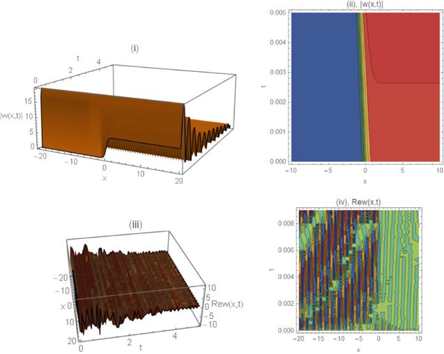
By using (11) and (18) ∣w(x, t)∣ and Re w(x, t) are evaluated and the numerical results are shown in figures 4(i)–(iv).
Figure 4. The 3D and contour plots of ∣w(x, t)∣ are displayed against x and t in figures 1(i) and (ii) respectively. The same is done for Rew(x, t) in figures 4(iii) and (iv) respectively. |
When β = −1.5, γ = 0.8, k = 4, h1 = 0.9, α = 1.9, c1 = 3.5, A0 = 1.5, s0 = 1.5, s1 = 2, $\mu (t)={\rm{{\rm{sech}} }}(0.06t+0.3)(3\sin (7t)+4\cos (8t))$. Figure 4(i) shows solitons cascade in time with self-steepening for small-time values. Figure 4(ii) shows significant self-steepening for small-time values. Figure 4(iii) shows quasi-self-modulation solitons in time. Figure 4 (iv) shows quasi-self modulation on x < 0 and for small-time values.
5. Discussion
The results found here are shown in the figures. These figures show the relevant behavior of solutions which are interpreted as self-steepening, self-phase modulation and high dispersivity in agreement with the characteristics of the perturbed NLSE.
Furthermore, different pattern formations are observed, solitons-cascade, complex waves, and rhombus shape.
6. Modulation instability
For analyzing the modulation instability (MI), an initial normal mode (NM) propagation is considered. Or also, when the NM is a possible pulse propagation in the system under study. Here, (1) admits a solution in the form,
$\begin{eqnarray}\begin{array}{rcl}w(x,t) & = & {A}_{0}{{\rm{e}}}^{{\rm{i}}({kx}-\omega t)},\\ {w}^{* }(x,t) & = & {A}_{0}{{\rm{e}}}^{-{\rm{i}}({kx}-\omega t)},{A}_{0}\gt 0,\,\\ \omega & = & -{A}_{0}^{2}({h}_{2}-k\beta )+{h}_{1}{k}^{2}+{k}^{3}\alpha .\end{array}\end{eqnarray}$
In (23) A0 is the amplitude. We consider, $\begin{eqnarray}\begin{array}{rcl}w(x,t) & = & {{\rm{e}}}^{{\rm{i}}({kx}-\omega t)}({A}_{0}+{\varepsilon }_{1}{{\rm{e}}}^{\lambda t}(U(X)+{\rm{i}}V(x)),\\ {w}^{* }(x,t) & = & {{\rm{e}}}^{-{\rm{i}}({kx}-\omega t)}({A}_{0}+{\varepsilon }_{2}{{\rm{e}}}^{\lambda t}(U(X)-{\rm{i}}V(x)).\end{array}\end{eqnarray}$
By inserting (24) into (1), calculations give rise to,
$\begin{eqnarray}\begin{array}{l}H\left(\begin{array}{c}{\varepsilon }_{1}\\ {\varepsilon }_{2}\end{array}\right)\,=\,0,\,H=\left(\begin{array}{cc}{a}_{11} & {a}_{12}\\ {a}_{21} & {a}_{22}\end{array}\right),\\ \quad {a}_{11}=\lambda U(x)+(k(2{h}_{1}+3k\setminus \alpha )\\ \quad -\,{A}_{0}^{2}(3\beta +2\gamma )){U}^{{\prime} }(x)-\alpha {U}^{(3)}(x),\\ {a}_{12}=(-{k}^{2}({h}_{1}+k\alpha )+{A}_{0}^{2}({h}_{2}+k\beta )\\ \quad +\,\omega V(x)+({h}_{1}+3k\alpha ){V}^{{\prime\prime} }(x),\\ \quad {a}_{21}=(-{k}^{2}({h}_{1}+k\alpha )+3{A}_{0}^{2}({h}_{2}+k\beta )\\ \quad +\,\omega )U(x)+({h}_{1}+3k\alpha ){U}^{{\prime\prime} }(x),\\ \quad {a}_{22}=\lambda V(x)+(2{h}_{1}k+3{k}^{2}\alpha \\ \quad -\,{A}_{0}^{2}\beta ){V}^{{\prime} }(x)-\alpha {V}^{(3)}(x).\end{array}\end{eqnarray}$
The eigenvalue problem is governed by the equation detH = 0, which gives rise to,
$\begin{eqnarray}{a}_{11}{a}_{22}-{a}_{12}{a}_{21}=0.\end{eqnarray}$
The eigenvalue problem in (26) is subjected to the boundary conditions U( ± ∞ ) = 0 and V( ± ∞ )) = 0. These conditions suggest to write,
$\begin{eqnarray}\left(\begin{array}{c}U(x)\\ V(x)\end{array}\right)=\left(\begin{array}{c}{A}_{1}\\ {A}_{2}\end{array}\right)\left\{\begin{array}{ll}{{\rm{e}}}^{-{mx}}, & x\gt 0,\,m\gt 0\\ {{\rm{e}}}^{{mx}} & x\lt 0,\,m\gt 0\end{array}.\right.\end{eqnarray}$
By substituting from (25) and (27) into (26), we find the eigenvalues,
$\begin{eqnarray}\begin{array}{rcl}\lambda & = & 2{h}_{1}{km}+3{k}^{2}m\alpha -{m}^{3}\alpha \\ & & -2{A}_{0}^{2}m\beta -{A}_{0}^{2}m\gamma \pm \sqrt{G},\\ G & = & -{m}^{4}{\left({h}_{1}+3k\alpha \right)}^{2}-{A}_{0}^{2}{m}^{2}(2{h}_{1}({h}_{2}+k\beta )\\ & & +3k\alpha (2{h}_{2}+2k\beta ))+{A}_{0}^{4}{m}^{2}{\left(\beta +\gamma \right)}^{2}.\end{array}\end{eqnarray}$
In (28), whatever the sign of G, we find that MI holds when,
$\begin{eqnarray}(\gamma +2\beta )\gt \displaystyle \frac{\alpha (-3{k}^{2}+{m}^{2})}{{A}_{0}^{2}},\alpha ,\beta ,\gamma \gt 0.\end{eqnarray}$
Thus (29) determines the critical value for the coefficient of self steepening (SS) (or the self-phase modulation (SPM)) to be dominant. This holds, provided that $m\gt \sqrt{3}$∣k∣. Alternatively, MI riggers the outbreak of SS (or SPM). dominates when $m\lt \sqrt{3}$∣k∣ high dispersivity occurs.7. Conclusions
Here, similariton solutions of the perturbed nonlinear Shrodinger equation are found. To this issue, similarity transformations are introduced. Further, a transformation that inspects the kinds of waves produced by soliton–periodic wave collision is applied. Exact solutions are obtained by using the extended unified method. The numerical results of the solution are shown graphically. These figures reveal self-steepening which progresses to a shock soliton in space for the intensity of the pulses, while the real part of the solutions shows self-phase modulation in time. Further, there are different patterns among them including soliton-cascades, complexes, rhombuses, and superlattices are remarked. It is also found that modulation instability is launched when the coefficients of self-steepening (self-modulation) exceed a critical value, which induces self-steepening phenomena. In future work, the behavior of similariton solutions of the perturbed Chen–Lee–Liu equation will be considered.
The author declares that there is no conflict of interest.