


1. Introduction
The Sine-Gordon equation (SGE) arose widely in physics and mathematics, such as in solutions with damping and a mixture of two types of driving force [1], the pinning transition [2], the homoclinic orbits [3], the exact Jacobian elliptic function solutions [4], a physics-constrained deep residual network [5], the tanh method and a variable separated ODE method [6], the slope modulation [7], the kinks bounded by fermions [8], the steady one-dimensional domain wall motion in biaxial ferromagnets [9], the observer-based boundary control of the energy [10] and the finite volume expectation values [11]. Also, there were plenty of researchers who devoted themselves to studying the properties of solitons and breathers of SGE. It has been given a complete categorization of solitons and their degenerate cases [12]. Currie executed a computer simulation program to study the dynamical behavior of solitons under external perturbations [13]. A direct approach was proposed to study soliton perturbations [14]. Breathers on potentials shipped with their scattering were taken into account [15, 16]. SGE was proved to possess the bounded state for breather–soliton molecules and breather molecules [17]. As far as we know, concerning the deductions of positons of SGE, Jaworski put forward a limiting method to derive a first-order positon [18], and an nth-order positon has been generated by Darboux transformation [19].
It is well-known that the higher-order smooth positons and breather positons are constructed by multi-solitons. In recent years, nth-order smooth positons and breather positons of modified Korteweg–de Vries (mKdV) equation have been constructed by means of Hirota’s bilinear method [20, 22], and the soliton molecules were also obtained by a new resonance condition in the muti-solitons [21]. Up to now, no one has constructed an nth-order smooth positon and a breather positon of SGE based on the bilinear method [22]. Thus, how to derive higher-order smooth positons and breather positons from the N-soliton solution is a noteworthy problem.
Aimed at solving this problem, our research studies the SGE as follows:2 ). Furthermore, this 1-positon was restricted with pure imaginary parameters λj [18].
$\begin{eqnarray}{u}_{{xt}}=4\sin u.\end{eqnarray}$
By means of Hirota’s bilinear method, the N-soliton solution of SGE is represented as $\begin{eqnarray}u\left(x,t\right)=2\mathrm{iln}\left(\displaystyle \frac{g}{f}\right),\end{eqnarray}$
where $\begin{eqnarray}\begin{array}{rcl}g & = & \displaystyle \sum _{\mu =0,1}\exp \left(\displaystyle \sum _{j\leqslant s}^{N}{\mu }_{j}{\mu }_{s}{A}_{{js}}+\displaystyle \sum _{j=1}^{N}{\mu }_{j}\left({\eta }_{j}-{\rm{i}}\displaystyle \frac{\pi }{2}\right)\right),\\ f & = & \displaystyle \sum _{\mu =0,1}\exp \left(\displaystyle \sum _{j\leqslant s}^{N}{\mu }_{j}{\mu }_{s}{A}_{{js}}+\displaystyle \sum _{j=1}^{N}{\mu }_{j}\left({\eta }_{j}+{\rm{i}}\displaystyle \frac{\pi }{2}\right)\right),\end{array}\end{eqnarray}$
with the abbreviation $\begin{eqnarray}\begin{array}{rcl}\exp \left({A}_{{js}}\right) & = & {\left(\displaystyle \frac{{\lambda }_{j}-{\lambda }_{s}}{{\lambda }_{j}+{\lambda }_{s}}\right)}^{2},\\ {\eta }_{j} & = & 2\left({\lambda }_{j}x+\displaystyle \frac{t}{{\lambda }_{j}}\right)+{\xi }_{j}^{\left(0\right)}.\end{array}\end{eqnarray}$
In a limiting case of the well-known 2-soliton solution, Jaworski just derived the first-order positons from equation (Getting rid of the preceding confines, this paper puts forward a tremendously appropriate limit method to figure out higher-order smooth positons and breather positons from equation (2 ). To a greatly practicable extent, the appropriate limit plays a dominant role without using any restrictive assumptions. Besides, by comparing the results produced by this limit method with those deduced by the Darboux transformation, we can clearly see the merits of the approach proposed in this paper.
2. Higher-order smooth positon
In this section, we initially generalize the derivation idea of first-order smooth positons of SGE [18]. Based on the approach of obtaining first-order smooth positons, we expand this idea to obtain second-order smooth positons and third-order positons only by adjusting parameters slightly. If the pattern continues, the construction of higher-order smooth positons pays off.
From the perspective of [18], for N = 2, they primarily assumed λj imaginary (namely λj = iνj, here νj are in real domain) and then ${\xi }_{j}^{\left(0\right)}=\mathrm{ln}\left(\tfrac{{\nu }_{1}+{\nu }_{2}}{{\nu }_{1}-{\nu }_{2}}\right)$. When ν2 → ν1, they obtained first-order positons via the limit of the standard 2-soliton formula. It is obvious that the limiting procedures discussed there can not apply to the nth-order smooth positon and real domain. In order to compensate for the regret, we refine and complete these frameworks into the following illustrations.
For N = 2, if some of the parameters in equation (
$\begin{eqnarray}{\lambda }_{2}={\lambda }_{1}+\epsilon ,\quad {\xi }_{1}^{\left(0\right)}=\mathrm{ln}\left(\displaystyle \frac{-\beta }{\epsilon }\right),\quad {\xi }_{2}^{\left(0\right)}=\mathrm{ln}\left(\displaystyle \frac{\beta }{\epsilon }\right),\end{eqnarray}$
then a first-order smooth positon ${u}_{1-p}$ will be obtained from the 2-soliton solution with the limit of $\epsilon \to 0$, and its mathematical formulation is $\begin{eqnarray}{u}_{1-p}=2\mathrm{iln}\left(\displaystyle \frac{g}{f}\right),\end{eqnarray}$
where $\begin{eqnarray}\begin{array}{rcl}g & = & 1+\beta {\partial }_{{\lambda }_{1}}{{\rm{e}}}^{{\xi }_{1}-{\rm{i}}\tfrac{\pi }{2}}-{B}_{11}{\beta }^{2}{{\rm{e}}}^{2{\xi }_{1}-{\rm{i}}\pi },\\ f & = & 1+\beta {\partial }_{{\lambda }_{1}}{{\rm{e}}}^{{\xi }_{1}+{\rm{i}}\tfrac{\pi }{2}}-{B}_{11}{\beta }^{2}{{\rm{e}}}^{2{\xi }_{1}+{\rm{i}}\pi },\end{array}\end{eqnarray}$
with the abbreviation $\begin{eqnarray}\begin{array}{rcl}{\xi }_{j} & = & 2\left({\lambda }_{j}x+\displaystyle \frac{t}{{\lambda }_{j}}\right),\\ {B}_{{\text{}}{js}} & = & \left\{\begin{array}{ll}\displaystyle \frac{1}{4{\lambda }_{j}^{2}}, & j=s,\\ {\left(\displaystyle \frac{{\lambda }_{j}-{\lambda }_{s}}{{\lambda }_{j}+{\lambda }_{s}}\right)}^{2}, & j\ne s.\end{array}\right.\end{array}\end{eqnarray}$
Here λj, β are all real parameters.
From equation (
$\begin{eqnarray}\begin{array}{rcl}g & = & 1-\displaystyle \frac{\beta }{\epsilon }{{\rm{e}}}^{\tfrac{2t}{{\lambda }_{1}}+2\,{\lambda }_{1}x-{\rm{i}}\displaystyle \frac{\pi }{2}}+\displaystyle \frac{\beta }{\epsilon }{{\rm{e}}}^{\tfrac{2t}{{\lambda }_{1}+\epsilon }+2\left({\lambda }_{1}+\epsilon \right)x-{\rm{i}}\displaystyle \frac{\pi }{2}}\\ & & -\displaystyle \frac{{\beta }^{2}}{4\,{\lambda }_{1}^{2}}{{\rm{e}}}^{\tfrac{2t}{{\lambda }_{1}}+2\,{\lambda }_{1}x+\displaystyle \frac{2t}{{\lambda }_{1}+\epsilon }+2\left({\lambda }_{1}+\epsilon \right)x-{\rm{i}}\pi },\end{array}\end{eqnarray}$
then in the limiting case of $\epsilon \to 0$, it leads to $\begin{eqnarray}\begin{array}{rcl}g & = & 1+\beta {\partial }_{{\lambda }_{1}}{{\rm{e}}}^{\tfrac{2t}{{\lambda }_{1}}+2\,{\lambda }_{1}x-{\rm{i}}\displaystyle \frac{\pi }{2}}\\ & & -\displaystyle \frac{{\beta }^{2}}{4{\lambda }_{1}^{2}}{{\rm{e}}}^{\tfrac{4t}{{\lambda }_{1}}+4\,{\lambda }_{1}x-{\rm{i}}\pi }.\end{array}\end{eqnarray}$
In the same way, f in equation ( $\begin{eqnarray}\begin{array}{rcl}f & = & 1+\beta {\partial }_{{\lambda }_{1}}{{\rm{e}}}^{\tfrac{2t}{{\lambda }_{1}}+2\,{\lambda }_{1}x+{\rm{i}}\displaystyle \frac{\pi }{2}}\\ & & -\displaystyle \frac{{\beta }^{2}}{4{\lambda }_{1}^{2}}{{\rm{e}}}^{\tfrac{4t}{{\lambda }_{1}}+4\,{\lambda }_{1}x+{\rm{i}}\pi }.\end{array}\end{eqnarray}$
Hence, equation (As is shown in the figure 1, when β > 0, the derivative value of the positon solution hits the maximum at a point. In this case, we obtain a bright first-order smooth positon. Conversely, a dark first-order smooth positon is derived like the case of β < 0.

Figure 1. A first-order smooth positon generated by equation ( |
For N = 3, if some of the parameters in equation (
$\begin{eqnarray}\begin{array}{rcl}{\lambda }_{2} & = & {\lambda }_{1}+\epsilon ,\quad {\lambda }_{3}={\lambda }_{1}+2\epsilon ,\quad {\xi }_{1}^{\left(0\right)}=\mathrm{ln}\left(\displaystyle \frac{\beta }{{\epsilon }^{2}}\right),\\ {\xi }_{2}^{\left(0\right)} & = & \mathrm{ln}\left(\displaystyle \frac{-2\beta }{{\epsilon }^{2}}\right),\\ {\xi }_{3}^{\left(0\right)} & = & \mathrm{ln}\left(\displaystyle \frac{\beta }{{\epsilon }^{2}}\right),\end{array}\end{eqnarray}$
then a second-order smooth positon ${u}_{2-p}$ will be obtained from the 3-soliton solution with the limit of $\epsilon \to 0$, and its mathematical formulation is $\begin{eqnarray}{u}_{2-p}=2\mathrm{iln}\left(\displaystyle \frac{g}{f}\right),\end{eqnarray}$
where $\begin{eqnarray}\begin{array}{rcl}g & = & 1+\beta {\left({\partial }_{{\lambda }_{1}}{\xi }_{1}\right)}^{2}{{\rm{e}}}^{{\xi }_{1}-{\rm{i}}\tfrac{\pi }{2}}+\beta {\partial }_{{\lambda }_{1}}^{2}{{\rm{e}}}^{{\xi }_{1}-{\rm{i}}\tfrac{\pi }{2}}\\ & & -\displaystyle \frac{{\beta }^{2}}{2}\left(4{B}_{11}{\left({\partial }_{{\lambda }_{1}}{\xi }_{1}\right)}^{2}-4{B}_{11}{\partial }_{{\lambda }_{1}}^{2}{\xi }_{1}+4\left({\partial }_{{\lambda }_{1}}{B}_{11}\right)\left({\partial }_{{\lambda }_{1}}{\xi }_{1}\right)\right.\\ & & \left.+{\partial }_{{\lambda }_{1}}^{2}{B}_{11}\right){{\rm{e}}}^{2{\xi }_{1}-{\rm{i}}\pi }-8{\beta }^{3}{B}_{11}^{3}{{\rm{e}}}^{3{\xi }_{1}-{\rm{i}}\tfrac{3\pi }{2}},\\ f & = & 1+\beta {\left({\partial }_{{\lambda }_{1}}{\xi }_{1}\right)}^{2}{{\rm{e}}}^{{\xi }_{1}+{\rm{i}}\tfrac{\pi }{2}}+\beta {\partial }_{{\lambda }_{1}}^{2}{{\rm{e}}}^{{\xi }_{1}+{\rm{i}}\tfrac{\pi }{2}}\\ & & -\displaystyle \frac{{\beta }^{2}}{2}\left(4{B}_{11}{\left({\partial }_{{\lambda }_{1}}{\xi }_{1}\right)}^{2}-4{B}_{11}{\partial }_{{\lambda }_{1}}^{2}{\xi }_{1}+4\left({\partial }_{{\lambda }_{1}}{B}_{11}\right)\left({\partial }_{{\lambda }_{1}}{\xi }_{1}\right)\right.\\ & & \left.+{\partial }_{{\lambda }_{1}}^{2}{B}_{11}\right){{\rm{e}}}^{2{\xi }_{1}+{\rm{i}}\pi }-8{\beta }^{3}{B}_{11}^{3}{{\rm{e}}}^{3{\xi }_{1}+{\rm{i}}\tfrac{3\pi }{2}}.\end{array}\end{eqnarray}$
ξ1 and Bjs have been presented in proposition 2.1 Here λj, β are all real parameters. Actually, the proof of proposition 2.2 is akin to that of proposition 2.1 . Although more complicatedly, it turns out as we intended. Figure 2(a) presents that a bright second-order smooth positon is generated when β > 0. When β < 0, we obtain a dark smooth positon. The judgment method is the same as the first-order smooth positon.

Figure 2. A second-order smooth positon generated by equation ( |
For N = 4, if some of the parameters in equation (
$\begin{eqnarray}\begin{array}{rcl}{\lambda }_{2} & = & {\lambda }_{1}+\epsilon ,\quad {\lambda }_{3}={\lambda }_{1}+2\epsilon ,\\ {\lambda }_{4} & = & {\lambda }_{1}+3\epsilon ,\\ {\xi }_{1}^{\left(0\right)} & = & \mathrm{ln}\left(\displaystyle \frac{-\beta }{{\epsilon }^{3}}\right),\quad {\xi }_{2}^{\left(0\right)}=\mathrm{ln}\left(\displaystyle \frac{3\beta }{{\epsilon }^{3}}\right),\\ {\xi }_{3}^{\left(0\right)} & = & \mathrm{ln}\left(\displaystyle \frac{-3\beta }{{\epsilon }^{3}}\right),\quad {\xi }_{4}^{\left(0\right)}=\mathrm{ln}\left(\displaystyle \frac{\beta }{{\epsilon }^{3}}\right),\end{array}\end{eqnarray}$
then a third-order smooth positon ${u}_{3-p}$ will be obtained from the 4-soliton solution with the limit of $\epsilon \to 0$, and its mathematical formulation is $\begin{eqnarray}{u}_{3-p}=2\mathrm{iln}\left(\displaystyle \frac{g}{f}\right),\end{eqnarray}$
where $\begin{eqnarray}\begin{array}{rcl}g & = & 1+\beta {\partial }_{{\lambda }_{1}}^{3}{{\rm{e}}}^{{\xi }_{1}-{\rm{i}}\tfrac{\pi }{2}}+{\omega }_{1}{{\rm{e}}}^{2{\xi }_{1}-{\rm{i}}\pi }\\ & & +{\omega }_{2}{{\rm{e}}}^{3{\xi }_{1}-{\rm{i}}\tfrac{3\pi }{2}}+1296{\beta }^{4}{B}_{11}^{6}{{\rm{e}}}^{4{\xi }_{1}-2{\rm{i}}\pi },\\ f & = & 1+\beta {\partial }_{{\lambda }_{1}}^{3}{{\rm{e}}}^{{\xi }_{1}+{\rm{i}}\tfrac{\pi }{2}}+{\omega }_{1}{{\rm{e}}}^{2{\xi }_{1}+{\rm{i}}\pi }\\ & & +{\omega }_{2}{{\rm{e}}}^{3{\xi }_{1}+{\rm{i}}\tfrac{3\pi }{2}}+1296{\beta }^{4}{B}_{11}^{6}{{\rm{e}}}^{4{\xi }_{1}+2{\rm{i}}\pi },\end{array}\end{eqnarray}$
with the abbreviation $\begin{eqnarray}\begin{array}{rcl}{\omega }_{1} & = & 3{\beta }^{2}\left[\Space{0ex}{2.9ex}{0ex}-{B}_{11}{\left({\partial }_{{\lambda }_{1}}{\xi }_{1}\right)}^{4}-3{B}_{11}{\left({\partial }_{{\lambda }_{1}}^{2}{\xi }_{1}\right)}^{2}\right.\\ & & +2{B}_{11}\left({\partial }_{{\lambda }_{1}}{\xi }_{1}\right)\left({\partial }_{{\lambda }_{1}}^{3}{\xi }_{1}\right)-2\left({\partial }_{{\lambda }_{1}}{B}_{11}\right){\left({\partial }_{{\lambda }_{1}}{\xi }_{1}\right)}^{3}\\ & & -\displaystyle \frac{3}{2}\left({\partial }_{{\lambda }_{1}}^{2}{B}_{11}\right){\left({\partial }_{{\lambda }_{1}}{\xi }_{1}\right)}^{2}-\displaystyle \frac{1}{2}\left({\partial }_{{\lambda }_{1}}^{3}{B}_{11}\right)\left({\partial }_{{\lambda }_{1}}{\xi }_{1}\right)\\ & & \left.+\left({\partial }_{{\lambda }_{1}}^{3}{\xi }_{1}\right)\left({\partial }_{{\lambda }_{1}}{B}_{11}\right)-\displaystyle \frac{1}{16}\left({\partial }_{{\lambda }_{1}}^{4}{B}_{11}\right)\right],\\ {\omega }_{2} & = & -18{B}_{11}{\beta }^{3}\left[2{B}_{11}^{2}{\partial }_{{\lambda }_{1}}^{3}{\xi }_{1}-6{B}_{11}\left({\partial }_{{\lambda }_{1}}{\xi }_{1}\right)\left({\partial }_{{\lambda }_{1}}^{2}{\xi }_{1}\right)\right.\\ & & +6{B}_{11}\left({\partial }_{{\lambda }_{1}}{B}_{11}\right){\left({\partial }_{{\lambda }_{1}}{\xi }_{1}\right)}^{2}+2{B}_{11}^{2}\left({\partial }_{{\lambda }_{1}}^{3}{\xi }_{1}\right)\\ & & -6{B}_{11}\left({\partial }_{{\lambda }_{1}}{B}_{11}\right)\left({\partial }_{{\lambda }_{1}}^{2}{\xi }_{1}\right)+6{\left({\partial }_{{\lambda }_{1}}{B}_{11}\right)}^{2}\left({\partial }_{{\lambda }_{1}}{\xi }_{1}\right)\\ & & \left.-{B}_{11}\left({\partial }_{{\lambda }_{1}}^{3}{B}_{11}\right)+3\left({\partial }_{{\lambda }_{1}}{B}_{11}\right)\left({\partial }_{{\lambda }_{1}}^{2}{B}_{11}\right)\right].\end{array}\end{eqnarray}$
ξ1 and Bjs have been presented in proposition 2.1 . Here λj, β are all real parameters. Obviously, when β > 0, the third-order positon is bright. Otherwise, when β < 0, we obtain a dark positon. Coincidentally, this phenomenon exists in both first-order smooth positon and second-order smooth positon.
If some of the parameters in equation (
$\begin{eqnarray}\begin{array}{rcl}{\lambda }_{2} & = & {\lambda }_{1}+\epsilon ,\quad {\lambda }_{3}={\lambda }_{1}+2\epsilon ,\\ {\lambda }_{4} & = & {\lambda }_{1}+3\epsilon ,\,\ldots \,,\quad {\lambda }_{N}={\lambda }_{1}+\left(N-1\right)\epsilon ,\\ {\xi }_{1}^{\left(0\right)} & = & \mathrm{ln}\displaystyle \frac{{\left(-1\right)}^{N+1}{C}_{N-1}^{0}\beta }{{\epsilon }^{N-1}},\\ {\xi }_{2}^{\left(0\right)} & = & \mathrm{ln}\displaystyle \frac{{\left(-1\right)}^{N+2}{C}_{N-1}^{1}\beta }{{\epsilon }^{N-1}},\\ {\xi }_{3}^{\left(0\right)} & = & \mathrm{ln}\displaystyle \frac{{\left(-1\right)}^{N+3}{C}_{N-1}^{2}\beta }{{\epsilon }^{N-1}},\,\ldots \,,\\ {\xi }_{N}^{\left(0\right)} & = & \mathrm{ln}\displaystyle \frac{{\left(-1\right)}^{2N}{C}_{N-1}^{N-1}\beta }{{\epsilon }^{N-1}},\end{array}\end{eqnarray}$
then a $\left(N-1\right)$ th-order smooth positon ${u}_{N-1-p}$ will be obtained from the N-soliton solution with the limit of $\epsilon \to 0$. Here λj, β are all real parameters.The results generated by this method can restore the results of the Darboux transformation. In contrast to the Darboux transformation, it is much more succinct to obtain higher-order smooth positons via inference 2.4 . In the case of utilizing the Darboux transformation, the arithmetic of Nth-order determinants is tedious.
According to the variance from figures 1 to 3, we get insight that first/second/third-order smooth positons can be categorized as bright and dark. Whereas, Darboux transformation has no observation in this regard. In [18], the parameters λj of equation (4 ) were restricted to pure imaginary, however the approach in this paper extends λj to the real domain. These are the new discoveries in the process of figuring out a higher-order smooth positon of SGE. Regrettably, we can not derive a general mathematical formulation of an nth-order smooth positon.

Figure 3. A third-order smooth positon generated by equation ( |
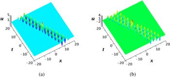
Figure 4. (a) A second-order breather positon derived with β = 2, λ1 = 1 + i, λ3 = 1 − i; (b) A third-order breather positon derived with β = 2, λ1 = 1 + i, λ4 = 1 − i. |
3. Higher-order breather positons
In this section, a flexible approach developed by [20] is employed to derive higher-order breather positons of SGE. It is a generally acknowledged truth that the parameters ηj of a nth-order breather positon must satisfy the condition: ${\eta }_{1}={\eta }_{n+1}^{* }$. In equation (4 ), this condition holds when ${\lambda }_{1}={\lambda }_{n+1}^{* }$, ${\xi }_{1}^{(0)}={\xi }_{n\,+\,1}^{(0)* }$. Here ${\xi }_{1}^{(0)}$, ${\xi }_{n+1}^{(0)}$ are in the real domain. We combine the requirements of the parameters above to obtain higher-order breather positons of SGE. It is a simple but skillful idea. We refine and complete this idea into the following illustrations.
For N = 4, if some of the parameters in equation (
$\begin{eqnarray}\begin{array}{rcl}{\lambda }_{2} & = & {\lambda }_{1}+\epsilon ,\quad {\xi }_{1}^{\left(0\right)}=\mathrm{ln}\left(\displaystyle \frac{-\beta }{\epsilon }\right),\\ {\xi }_{2}^{\left(0\right)} & = & \mathrm{ln}\left(\displaystyle \frac{\beta }{\epsilon }\right),\\ {\lambda }_{4} & = & {\lambda }_{3}+\epsilon ,\quad {\xi }_{3}^{\left(0\right)}=\mathrm{ln}\left(\displaystyle \frac{-\beta }{\epsilon }\right),\\ {\xi }_{4}^{\left(0\right)} & = & \mathrm{ln}\left(\displaystyle \frac{\beta }{\epsilon }\right),\\ {\lambda }_{1} & = & {\lambda }_{3}^{* },\quad {\xi }_{1}={\xi }_{3}^{* },\end{array}\end{eqnarray}$
then a second-order breather positon ${u}_{2-{bp}}$ will be generated by the 4-soliton solution with the limit of $\epsilon \to 0$ and its mathematical formulation is $\begin{eqnarray}{u}_{2-{bp}}=2\mathrm{iln}\left(\displaystyle \frac{g}{f}\right),\end{eqnarray}$
where $\begin{eqnarray}\begin{array}{rcl}g & = & 1+\beta {\partial }_{{\lambda }_{1}}{{\rm{e}}}^{{\xi }_{1}-{\rm{i}}\tfrac{\pi }{2}}+\beta {\partial }_{{\lambda }_{3}}{{\rm{e}}}^{{\xi }_{3}-{\rm{i}}\tfrac{\pi }{2}}-{\beta }^{2}{B}_{11}{{\rm{e}}}^{2{\xi }_{1}-{\rm{i}}\pi }\\ & & -{\beta }^{2}{B}_{33}{{\rm{e}}}^{2{\xi }_{3}-{\rm{i}}\pi }+{\beta }^{2}{\partial }_{{\lambda }_{1}}{\partial }_{{\lambda }_{3}}{B}_{13}{{\rm{e}}}^{{\xi }_{1}+{\xi }_{3}-{\rm{i}}\pi }\\ & & +{\omega }_{1}{{\rm{e}}}^{2{\xi }_{1}+{\xi }_{3}-{\rm{i}}\tfrac{3\pi }{2}}+{\omega }_{2}{{\rm{e}}}^{{\xi }_{1}+2{\xi }_{3}-{\rm{i}}\tfrac{3\pi }{2}}\\ & & +{\beta }^{4}{B}_{11}{B}_{13}^{4}{B}_{33}{{\rm{e}}}^{2{\xi }_{1}+2{\xi }_{3}-2{\rm{i}}\pi },\\ f & = & 1+\beta {\partial }_{{\lambda }_{1}}{{\rm{e}}}^{{\xi }_{1}+{\rm{i}}\tfrac{\pi }{2}}+\beta {\partial }_{{\lambda }_{3}}{{\rm{e}}}^{{\xi }_{3}+{\rm{i}}\tfrac{\pi }{2}}-{\beta }^{2}{B}_{11}{{\rm{e}}}^{2{\xi }_{1}+{\rm{i}}\pi }\\ & & -{\beta }^{2}{B}_{33}{{\rm{e}}}^{2{\xi }_{3}+{\rm{i}}\pi }+{\beta }^{2}{\partial }_{{\lambda }_{1}}{\partial }_{{\lambda }_{3}}{B}_{13}{{\rm{e}}}^{{\xi }_{1}+{\xi }_{3}+{\rm{i}}\pi }\\ & & +{\omega }_{1}{{\rm{e}}}^{2{\xi }_{1}+{\xi }_{3}+{\rm{i}}\tfrac{3\pi }{2}}+{\omega }_{2}{{\rm{e}}}^{{\xi }_{1}+2{\xi }_{3}+{\rm{i}}\tfrac{3\pi }{2}}\\ & & +{\beta }^{4}{B}_{11}{B}_{13}^{4}{B}_{33}{{\rm{e}}}^{2{\xi }_{1}+2{\xi }_{3}+2{\rm{i}}\pi },\end{array}\end{eqnarray}$
with the abbreviation $\begin{eqnarray}\begin{array}{rcl}{\omega }_{1} & = & -{\beta }^{3}{B}_{13}{B}_{11}\left({B}_{13}{\partial }_{{\lambda }_{3}}{\xi }_{3}+2{\partial }_{{\lambda }_{3}}{B}_{13}\right),\\ {\omega }_{2} & = & -{\beta }^{3}{B}_{13}{B}_{33}\left({B}_{13}{\partial }_{{\lambda }_{1}}{\xi }_{1}+2{\partial }_{{\lambda }_{1}}{B}_{13}\right).\end{array}\end{eqnarray}$
Here ξj and Bjs have been written in proposition 2.1 . λj are all complex parameters, it is worth noting that ${\lambda }_{1}={\lambda }_{3}^{* }=a+{\rm{i}}b$ holds if and only if neither the real part nor the imaginary part of the λ1 is equal to zero. And β here is in the real domain. The result obtained is demonstrated graphically in figure 4(a). Analogous to proposition 3.1 , the following inference presents a concise way to derive higher-order breather positons like the third-order breather positon in figure 4(b).
For N = 2n, if some of the parameters in equation (
$\begin{eqnarray}\begin{array}{rcl}{\lambda }_{2} & = & {\lambda }_{1}+\epsilon ,\quad {\lambda }_{3}={\lambda }_{1}+2\epsilon ,\,\ldots \,,\\ {\lambda }_{n} & = & {\lambda }_{1}+\left(n-1\right)\epsilon ,\quad {\lambda }_{1}={\lambda }_{n+1}^{* },\\ {\lambda }_{n+2} & = & {\lambda }_{n+1}+\epsilon ,\quad {\lambda }_{n+3}={\lambda }_{n+1}+2\epsilon ,\,\ldots \,,\\ {\lambda }_{2n} & = & {\lambda }_{n+1}+\left(n-1\right)\epsilon ,\\ {\xi }_{1}^{\left(0\right)} & = & \mathrm{ln}\displaystyle \frac{{\left(-1\right)}^{n+1}{C}_{n-1}^{0}\beta }{{\epsilon }^{n-1}},\quad {\xi }_{2}^{\left(0\right)}=\mathrm{ln}\displaystyle \frac{{\left(-1\right)}^{n+2}{C}_{n-1}^{1}\beta }{{\epsilon }^{n-1}},\,\ldots \,,\\ {\xi }_{n}^{\left(0\right)} & = & \mathrm{ln}\displaystyle \frac{{\left(-1\right)}^{2n}{C}_{n-1}^{n-1}\beta }{{\epsilon }^{n-1}},\\ {\xi }_{n+1}^{\left(0\right)} & = & \mathrm{ln}\displaystyle \frac{{\left(-1\right)}^{n+1}{C}_{n-1}^{0}\beta }{{\epsilon }^{n-1}},\quad {\xi }_{n+2}^{\left(0\right)}=\mathrm{ln}\displaystyle \frac{{\left(-1\right)}^{n+2}{C}_{n-1}^{1}\beta }{{\epsilon }^{n-1}},\,\ldots \,,\\ {\xi }_{2n}^{\left(0\right)} & = & \mathrm{ln}\displaystyle \frac{{\left(-1\right)}^{2n}{C}_{n-1}^{n-1}\beta }{{\epsilon }^{n-1}},\end{array}\end{eqnarray}$
then a nth-order breather positon ${u}_{n-{bp}}$ will be generated by $2n$-soliton solution in the limit of $\epsilon \to 0$.4. Conclusion
According to the N-soliton solution generated by Hirota’s bilinear method, we exploit an ingenious limit method to obtain higher-order smooth positons and breather positons of SGE. In inference 2.4 and inference 3.2 , the essence of this technique is extracted and generalized. By means of this approach, the results generated by this method can restore the results of the Darboux transformation. Moreover, higher-order smooth positons can be categorized as bright and dark. In terms of feasibility and practicability, this approach provides new ideas for deriving higher-order smooth positons and breather positons of other integrable systems.
This new method expands the parameters λj of the higher-order smooth positon to the real domain, which gets rid of the constraint of pure imaginary parameters [18]. During the procedure of deduction, the approach in this paper has the strengths of concision and high efficiency, contrasting with the Darboux transformation. Whereas, we still need to make great efforts to deduce the general mathematical formulation of nth-order smooth positons and breather positons.