


1. Introduction
2. The IST with ZBCs and BS solution
2.1. The structure of the RH problem with ZBCs
$M(x,t,\lambda )$ solve the following RH problem
2.2. BS soliton with a higher-order pole
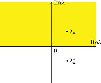
Figure 1. Depicts the contours and the discrete spectrum of the RH problem on complex λ-plane, ${{\mathbb{C}}}_{+}$ (yellow) and ${{\mathbb{C}}}_{-}$ (white). |
Based on the ZBCs at infinity provided in (
First, we introduce
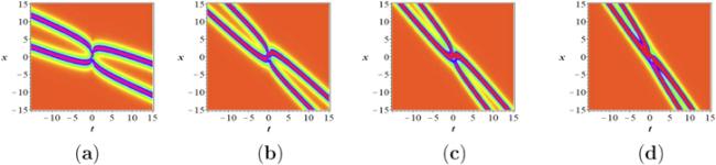
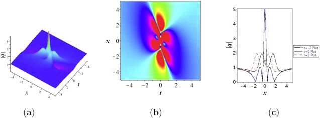
Figure 2. The density plots of the second-order the BS soliton solution ( |
3. The IST with NZBCs and RW
3.1. The structure of the RH problem with NZBCs
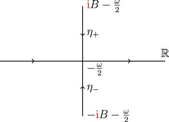
Figure 3. The contour ${{\rm{\Sigma }}}_{0}={\mathbb{R}}\cup \eta $ of the basic RH problem. |
$M(x,t,\lambda )$ solves the RH problem
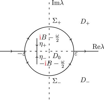
Figure 4. Definitions of the regions D±, D0 and Σ±, η. |
3.2. RW of the inhomogeneous fifth-order NLS equation
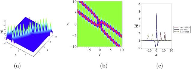
Figure 5. The temporal-spatial periodic breather wave solutions ( |

Figure 6. The spatial periodic breather wave solutions ( |
| a | (a) For c1 = − c2 = 1, we obtain the first-order RW solution as (see figure 7) $\begin{eqnarray}\widetilde{q}(x,t)=\left(B+\displaystyle \frac{4{B}^{2}[{\left(x+\delta t\right)}^{* }-(x+\delta t)]-4B}{{B}^{2}\left[1+2(x+\delta t)+2{\left(x+\delta t\right)}^{* }+4| x+\delta t{| }^{2}\right]+1}\right){{\rm{e}}}^{{\rm{i}}(\omega x+\nu t)}.\end{eqnarray}$ |
| b | (b) For ${{\boldsymbol{c}}}_{\infty }={\left(c,-c\right)}^{\top }$, we obtain the first-order RW solution with its (see figure 8) $\begin{eqnarray}\widetilde{q}(x,t)=\left(\displaystyle \frac{B\left[4{B}^{2}| x+\delta t{| }^{2}+4B{\left(x+\delta t\right)}^{* }-4B(x+\delta t)-3\right]}{4{B}^{2}| x+\delta t{| }^{2}+1}\right){{\rm{e}}}^{{\rm{i}}(\omega x+\nu t)}.\,\end{eqnarray}$ |
| c | (c) For c1 + c2 ≠ 0, e.g. ${c}_{1}=c+\tfrac{\varpi }{2}$, ${c}_{2}=-c+\tfrac{\varpi }{2}$ with $c\in {\mathbb{C}}\setminus \{0\}$ and ϖ ≪ 1. Let $x=\tfrac{\overline{x}}{| \varpi | },t=\tfrac{\overline{t}}{| \varpi | }$, if $(\overline{x},\overline{t})\in {{\mathbb{R}}}^{2}$ is fixed, and then we obtain $\begin{eqnarray}{\boldsymbol{s}}(x,t)=\left(\begin{array}{c}c+{{\rm{e}}}^{\mathrm{iarg}(\varpi )}B(\overline{x}+\delta \overline{t})\\ -c-{{\rm{e}}}^{\mathrm{iarg}(\varpi )}B(\overline{x}+\delta \overline{t})\end{array}\right)+O(\varpi ),\end{eqnarray}$ $\begin{eqnarray}\begin{array}{l}{ \mathcal N }=2| c{| }^{2}+4\mathrm{Re}\{{{Bc}}^{* }{{\rm{e}}}^{\mathrm{iarg}(\varpi )}(\overline{x}+\delta \overline{t})\}\\ \quad +2{B}^{2}({\overline{x}}^{2}+| \delta {| }^{2}{\overline{t}}^{2})+O(\varpi ),\end{array}\end{eqnarray}$ $\begin{eqnarray}\begin{array}{rcl}\vartheta & = & \displaystyle \frac{1}{| \varpi | }\left[-\displaystyle \frac{2}{3}{B}^{2}{{\rm{e}}}^{2\mathrm{iarg}(\varpi )}{\left(\overline{x}+\delta \overline{t}\right)}^{3}\right.\\ & & \left.-2{cB}{{\rm{e}}}^{\mathrm{iarg}(\varpi )}{\left(\overline{x}+\delta \overline{t}\right)}^{2}-2{c}^{2}(\overline{x}+\delta \overline{t})\right]+O(1).\end{array}\end{eqnarray}$ Further, we can get $\widetilde{q}(x,t)\approx 1$, unless the leading term in ϑ proportional to $\tfrac{1}{| \varpi | }$ is cancelled, these terms will form a cubic equation of ${\mathfrak{n}}=\overline{x}+\delta \overline{t}$, and its three roots are ${\mathfrak{n}}=0$ and $\tfrac{1}{2}c{\left(B\varpi \right)}^{-1}(-3\pm {\rm{i}}\sqrt{3})$, respectively (see figure 9). |
| d | (d) For ${{\boldsymbol{c}}}_{\infty }={\left(\mathrm{1,1}\right)}^{\top }$, we can obtain the second-order RW (see figure 10) $\begin{eqnarray}\widetilde{q}(x,t)=\left(B-12B\displaystyle \frac{{\mathfrak{P}}}{{\mathfrak{Q}}}\right){{\rm{e}}}^{{\rm{i}}(\omega x+\nu t)},\end{eqnarray}$ |
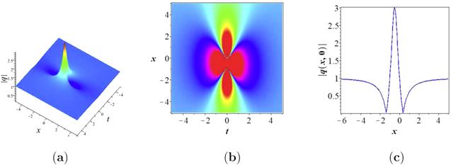
Figure 7. The first-order RW solutions ( |
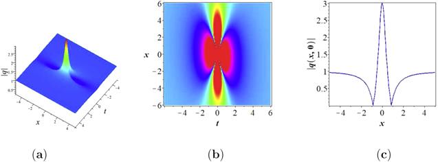
Figure 8. The first-order RW solutions ( |
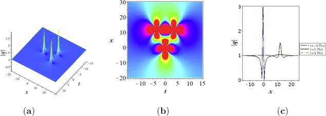
Figure 9. The first-order RW solutions ( |
Figure 10. The second-order RW solutions ( |