


1. Introduction
2. The methods
2.1. Scalar and electromagnetic field perturbations in quantum-corrected Schwarzschild black hole
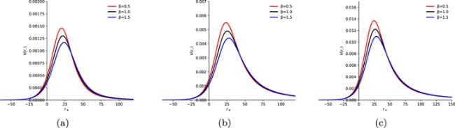
Figure 1. The effective potentials of the scalar field with the different l. (a) l = 0 (b) l = 1 (c) l = 2. |
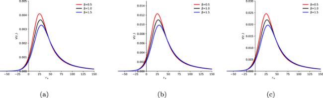
Figure 2. The effective potentials of the electromagnetic field with the different l. (a) l = 1 (b) l = 2 (c) l = 3. |
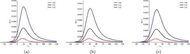
Figure 3. The effective potentials of the scalar field with the different β. (a) β = 0.5 (b) β = 1.0 (c) β = 1.5. |
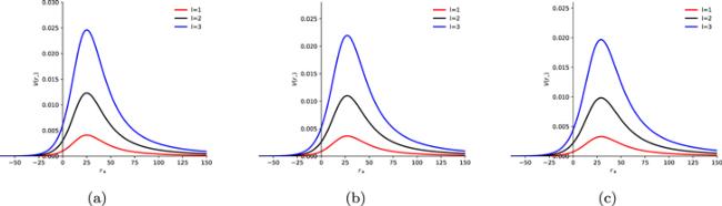
Figure 4. The effective potentials of the electromagnetic field with the different β. (a) β = 0.5 (b) β = 1.0 (c) β = 1.5. |
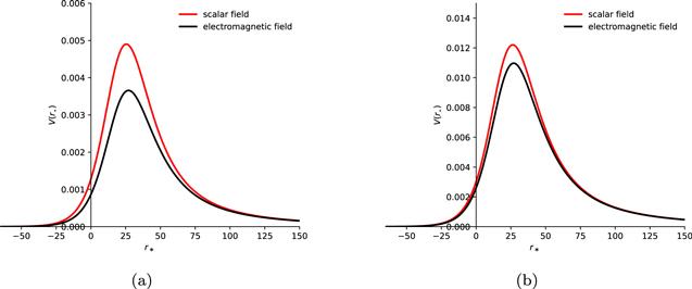
Figure 5. The effective potentials of the scalar and electromagnetic field. (a) β = 1, l = 1 (b) β = 1, l = 2. |
2.2. The WKB method
2.3. The time domain method
3. Quantum-corrected Schwarzschild black hole model
Table 1. The QNM frequencies of scalar field. |
| WKB method | ||||
|---|---|---|---|---|
| β | l = 0 | l = 1 | l = 2 | l = 3 |
| 0.25 | 0.026 779 – 0.024441i | 0.071 008 – 0.023699i | 0.117 247 – 0.023458i | 0.163 725 – 0.023394i |
| 0.50 | 0.025 991 – 0.023722i | 0.068 919 – 0.023002i | 0.113 798 – 0.022768i | 0.158 910 – 0.022706i |
| 0.75 | 0.025 248 – 0.023044i | 0.066 950 – 0.022345i | 0.110 547 – 0.022118i | 0.154 369 – 0.022057i |
| 1.00 | 0.024 547 – 0.022404i | 0.065 091 – 0.021724i | 0.107 476 – 0.021503i | 0.150 081 – 0.021444i |
| 1.25 | 0.023 885 – 0.021797i | 0.063 331 – 0.021130i | 0.104 571 – 0.020922i | 0.146 025 – 0.020865i |
| 1.50 | 0.023 255 – 0.021224i | 0.061 665 – 0.020581i | 0.101 819 – 0.020371i | 0.142 182 – 0.020315i |
Table 2. The QNM frequencies of electromagnetic field. |
| WKB method | ||||
|---|---|---|---|---|
| β | l = 1 | l = 2 | l = 3 | l = 4 |
| 0.25 | 0.060 167 6 – 0.022457i | 0.110 932 – 0.023033i | 0.159 248 – 0.023179i | 0.206 811 – 0.023238i |
| 0.50 | 0.058 398 – 0.021796i | 0.107 669 – 0.022355i | 0.154 564 – 0.022498i | 0.200 728 – 0.022555i |
| 0.75 | 0.056 729 5 – 0.021174i | 0.104 593 – 0.021716i | 0.150 148 – 0.021855i | 0.194 993 – 0.021910i |
| 1.00 | 0.055 153 – 0.020586i | 0.101 687 – 0.021113i | 0.145 977 – 0.021248i | 0.189 577 – 0.021302i |
| 1.25 | 0.053 663 – 0.020029i | 0.098 939 – 0.020541i | 0.142 032 – 0.020674i | 0.184 453 – 0.020726i |
| 1.50 | 0.052 250 – 0.019502i | 0.096 335 – 0.020002i | 0.138 294 – 0.020129i | 0.179 599 – 0.020181i |
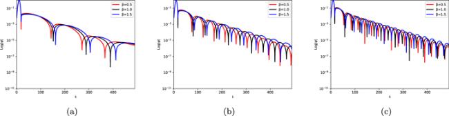
Figure 6. The dynamical evolutions of the scalar field with the different l. (a) l = 0 (b) l = 1 (c) l = 2. |
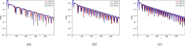
Figure 7. The dynamical evolutions of the electromagnetic field with the different l. (a) l = 1 (b) l = 2 (c) l = 3. |
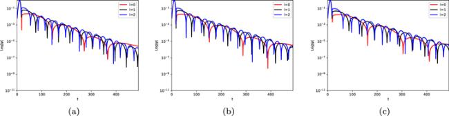
Figure 8. The dynamical evolutions of the scalar field with the different β. (a) β = 0.5 (b) β = 1.0 (c) β = 1.5. |
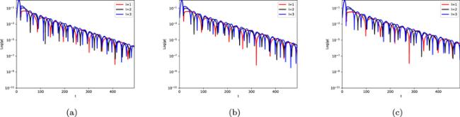
Figure 9. The dynamical evolutions of the electromagnetic field with the different β. (a) β = 0.5 (b) β = 1.0 (c) β = 1.5. |

Figure 10. The dynamical evolutions of the scalar and electromagnetic field. (a) β = 1, l = 1 (b) β = 1, l = 2. |
4. Conclusions
| 1. | (1) The effective potential of the GUP quantum-corrected Schwarzschild black hole decrease with the increase of β, and increase with the increase of l. When r* approaches infinity, the effective potential tends to 0 and the black hole will be unaffected by the change of parameters and finally comes back to the equilibrium state. |
| 2. | (2) The QNM ringing of the GUP quantum-corrected Schwarzschild black hole appears after the initial pulse. When l is fixed, the QNM oscillation becomes weaker as β increases, the correction term of GUP makes the black hole metric gauge not singular; when β is fixed, the QNM oscillation becomes stronger as l increases. It can be concluded that the trend of QNM is related to the effective potential. |
| 3. | (3) The QNM is a special characteristic of the solution of the black hole perturbation equation, which occupies the main time in the black hole perturbation process. The parameter l influences the perturbation time of QNM, among the most obvious in figure 6(a), which affects the spacetime with black hole background. In other words, it affects the intrinsic frequency as well as the damping rate of the oscillation and is not affected by the initial oscillation. |
| 4. | (4) In figures 6–7, when l is a constant value, the period of the time of QNM perturbation is β = 1.5 > β = 1.0 >β = 0.5, then β = 0.5 is easier to detect. In figure 8, it is known that whenever β is a constant value, the duration of the perturbation time is l = 0 > l = 1 > l = 2, then l = 2 is more easily detected. In figure 9, it is well recognized that as long as β is a constant, the length of the perturbation time is l = 1 > l = 2 > l = 3, then l = 3 is easy to be found. |
| 5. | (5) The average value of the ringing of QNM in scalar and electromagnetic fields is about in the range of 10−1 and 10−8, which is in agreement with our results in tables 1–2. |
| 6. | (6) The QNM ringing of the scalar is larger than that of the electromagnetic field field, which means that the radiation excited by the perturbation in the scalar field may be larger than that excited by the electromagnetic field field. |