The Hirota equation can be used to describe the wave propagation of an ultrashort optical field. In this paper, the multi-component Hirota (alias n-Hirota, i.e. n-component third-order nonlinear Schrödinger) equations with mixed non-zero and zero boundary conditions are explored. We employ the multiple roots of the characteristic polynomial related to the Lax pair and modified Darboux transform to find vector semi-rational rogon-soliton solutions (i.e. nonlinear combinations of rogon and soliton solutions). The semi-rational rogon-soliton features can be modulated by the polynomial degree. For the larger solution parameters, the first m (m < n) components with non-zero backgrounds can be decomposed into rational rogons and grey-like solitons, and the last n − m components with zero backgrounds can approach bright-like solitons. Moreover, we analyze the accelerations and curvatures of the quasi-characteristic curves, as well as the variations of accelerations with the distances to judge the interaction intensities between rogons and grey-like solitons. We also find the semi-rational rogon-soliton solutions with ultra-high amplitudes. In particular, we can also deduce vector semi-rational solitons of the n-component complex mKdV equation. These results will be useful to further study the related nonlinear wave phenomena of multi-component physical models with mixed background, and even design the related physical experiments.
Weifang Weng, Guoqiang Zhang, Shuyan Chen, Zijian Zhou, Zhenya Yan. Vector semi-rational rogon-solitons and asymptotic analysis for any multi-component Hirota equations with mixed backgrounds[J]. Communications in Theoretical Physics, 2022, 74(9): 095001. DOI: 10.1088/1572-9494/ac6799
1. Introduction
The study of solitons [1–5] and rogue waves (alias rogons [6]) [7–21] is still a significant topic in the field of nonlinear sciences. They can be used to describe the wave propagations and fundamental features of some nonlinear physical phenomena appearing in nonlinear optics, Bose–Einstein condensates, plasmas physics, quantum optics, DNA, fluid mechanics, ocean, and even finance. As a fundamental and universal physical model, the focusing nonlinear Schrödinger (NLS) equation is completely integrable [22], and admits the abundant nonlinear modes, such as the bright solitons, rogons, and breathers [7, 10, 14, 19, 20, 22]. As a type of higher-order extensions of the NLS equation, Hirota [23] further extended the NLS equation to first propose a third-order NLS equation (alias Hirota equation)
which is used to demonstrate the propagating wave of an ultrashort optical field p = p(x, t) in an optical fibre [24–26], where the subscripts denote the partial derivatives with respect to the variables x, t. Equation (1) was shown to be completely integrable, and to possess the solitons and rogons in terms of the bilinear method [23], the modified Darboux transform [27–30] and robust inverse scattering method [31]. Moreover, the inverse scattering and multi-pole solitons of equation (1) with non-zero boundary conditions were investigated [32, 33]. The multi-component nonlinear wave equations, as the extensions of the single NLS and Hirota equations, were also studied to analyze the interplays of many bodies. Recently, the vector rogons and semi-rational solutions were also found for the two-component coupled NLS equation [34–46] and three-component coupled NLS equations [47–49]. Moreover, the vector rogons and semi-rational solutions were also shown to appear in the two-component Hirota equations [50, 51], and three-component Hirota equation [52].
As the number n of components increases, the key and difficult point is how to find the explicit multiple eigenvalues of the (n + 1)-order matrix related to the Lax pairs of the n-component nonlinear wave equations. Recently, Zhang et al [53, 54] presented a powerful approach to studying this problem such that any n-component NLS equations and their higher-order extensions with non-zero backgrounds have been found to possess the novel vector rogons [55]. Moreover, we further extended this idea to obtain the semi-rational rogon-soliton solutions of 5-component Manakov equations [56], and even any n-component NLS equations [57]. These solutions imply the interplays of rational rogons and grey-like solitons, as well as ones of the bright-like solitons and localized small modes. To the best of our knowledge, the any n-component Hirota (third-order NLS) equations with n > 3 were not found to possess the semi-rational rogon-soliton solutions except for a few works on the 2-Hirota and 3-Hirota equations [50–52, 58].
The n-component Hirota (alias the n-Hirota) equations can be written as the dimensionless form [23, 55]
where p(x, t) = (p1(x, t), p2(x, t), …, pn(x, t))T$(n\in {\mathbb{N}})$ stands for an envelope vector field describing the n components in the nonlinear optical fibre, the subscripts denote the partial derivatives with respect to the variables x, t, and $^{\prime} \dagger ^{\prime} $ denotes the Hermitian conjugate. The n-Hirota equation (2) can be rewritten as
where the star denotes the complex conjugate. Equation (2) can be refereed to as the vector extension of equation (1), and reduces to the single Hirota equation (1) at n = 1, while equation (2) becomes the coupled Hirota equation and 3-Hirota equation at n = 2, 3, respectively. As α ≠ 0, ϵ = 0, equation (2) reduces to the n-component NLS (n-NLS) equation [59]. When α = 0, ϵ ≠ 0, equation (2) becomes the n-component complex mKdV (n-cmKdV) equation
which can deduce the ‘new' solutions of equation (2), where Φ(x, t; μ0) = (φ1(x, t; μ0), φ2 (x, t; μ0), …, φn+1 (x, t; μ0))T is a vector-function solution of the Lax pair (4) with p(x, t) = p0(x, t) and μ = μ0.
In this paper, we would like to study the semi-rational rogon-soliton solutions and asymptotic analysis of the n-Hirota equation (2) with the mixed non-zero and zero boundary conditions. The semi-rational rogon-soliton solutions can be decomposed into the interplays between the rogons and grey-like solitons. Moreover, the quasi-characteristic curves of the wave propagations of these grey-like solitons are almost the straight lines, which differ from ones of the n-NLS equation, which are the logarithmic function curves.
The rest of this paper is arranged as follows: in section 2, starting from the (n + 1)-order matrix Lax pair (4) with the initial plane-wave solutions (6), we find the explicit vector semi-rational rogon-soliton solutions of the n-Hirota equation by means of the modified Darboux transform, and the multiple eigenvalues of an (n + 1)-order matrix ${ \mathcal U }$. In section 3, we analyze the obtained wave structures and their asymptotics. In particular, the semi-rational rogon-soliton solutions can be decomposed into the rogons and grey-like solitons when the absolute values of some parameters become bigger. Moreover, we discuss the velocities and accelerations of wave propagations of the decomposed grey-like solitons, the curvatures of the quasi-characteristic curves of the grey-like solitons and the relations between the curvatures of the quasi-characteristic curves and the distances defined by from the center points into the points on the quasi-characteristic curves. In section 4, we study the parameter constraints for the vector semi-rational rogon-soliton solutions with ultra-high amplitudes. In section 5, the above-mentioned results can reduce to ones of the n-cmKdV equation at α = 0, ϵ ≠ 0. Particularly, we find the different vector semi-rational W-shaped soliton and grey-like solitons of the n-cmKdV equation. Finally, we present some conclusions and discussions in section 6.
2. Vector semi-rational rogon-soliton solutions of (2) with mixed backgrounds
Here to study the vector semi-rational rogon-soliton solutions of the n-Hirota equation (2) we start from its plane-wave solutions
where ${a}_{j},{b}_{j}\in {\mathbb{R}}$, ${\boldsymbol{a}}={\left({a}_{1},{a}_{2},\ldots ,{a}_{n}\right)}^{{\rm{T}}}$ and ∥a∥2 = aTa. Without loss of generality, one can take aj ≥ 0. Notice that as some as = 0 (s ∈ {1, 2,…,n}), the corresponding bs, νs can be chosen as any real constants. Of course, one can also take the νs given by equation (6). One can find the fundamental solutions of the Lax pair (4) with p = p0(x, t) given by equation (6) and μ = μ0
$\begin{eqnarray}\begin{array}{l}{\rm{\Phi }}(x,t;{\mu }_{0})=\mathrm{diag}\left(1,{{\rm{e}}}^{{\rm{i}}{\varphi }_{1}(x,t)},{{\rm{e}}}^{{\rm{i}}{\varphi }_{2}(x,t)},\cdots ,{{\rm{e}}}^{{\rm{i}}{\varphi }_{n}(x,t)}\right)\\ \times \exp \,\left({\rm{i}}\,{ \mathcal U }({\mu }_{0})x+\displaystyle \frac{{\rm{i}}}{2}g({ \mathcal U }({\mu }_{0}))t\right){\boldsymbol{c}}\end{array}\end{eqnarray}$
by means of the gauge transform $\Psi$ (x, t; μ0) = diag (1, ${{\rm{e}}}^{{\rm{i}}{\varphi }_{1}}$, ${{\rm{e}}}^{{\rm{i}}{\varphi }_{2}}$, …, ${{\rm{e}}}^{{\rm{i}}{\varphi }_{n}}$ ) Φ (x, t; μ0), where ${\boldsymbol{c}}={\left({c}_{0},{c}_{1},\ldots ,{c}_{n}\right)}^{{\rm{T}}}$ is a non-zero constant vector, and the matrix polynomial g (${ \mathcal U }$ (μ0)) = ϵ${{ \mathcal U }}^{3}$ (μ0) + (α + 3ϵμ0) ${{ \mathcal U }}^{2}$ (μ0) + [3ϵ$({\mu }_{0}^{2}-\parallel {\boldsymbol{a}}{\parallel }^{2})\,$ + 2αμ0] ${ \mathcal U }$ (μ0) − [3ϵ (${\mu }_{0}^{3}+\parallel {\boldsymbol{a}}{\parallel }^{2}$μ0 −$\,{\sum }_{s=1}^{n}{a}_{s}^{2}{b}_{s}$) + α(${\mu }_{0}^{2}+2\parallel {\boldsymbol{a}}{\parallel }^{2}$ )] ${{\mathbb{I}}}_{n+1}$ with ${ \mathcal U }$ (μ0) = μ0${{\mathbb{I}}}_{n+1}+\left(\begin{array}{cc}0 & {{\boldsymbol{a}}}^{{\rm{T}}}\\ {\boldsymbol{a}} & -B\end{array}\right)$, B = diag (b1, b2, …, bn).
To explore the vector semi-rational rogon-soliton solutions of the n-Hirota system (2), we should find the explicit multiple eigenvalues of ${ \mathcal U }({\mu }_{0})$. For the case aj ≠ 0, ak =0(j = 1, 2,…,m; k = m + 1,…,n; ⌈n/2⌉ ≤ m < n), we show that if the non-zero amplitudes aj and wavenumbers bj (j =1,…,m, ) and spectral parameter μ0 are given by aj = csc (j π/(m + 1)), bj = cot (jπ/(m + 1)), μ0 = i(m + 1)/2, j = 1, 2, …, m, and each bk(k = m + 1,…,n) is equal to one of bj (j = 1,…,m) with ${{\rm{\Pi }}}_{s,k=m+1}^{n}{\left({b}_{s}-{b}_{k}\right)}^{2}\ne 0$, then the matrix ${ \mathcal U }({\mu }_{0})$ possesses the (m + 1)-multiple root i(1 − m)/2 and (n − m) simple roots − (i(m + 1)/2 + bk)(k = m + 1,…,n).
Therefore, we, based on the above DT (5), equation (7), and the given aj, bj, μ0, have the following property:
The formula of vector semi-rational rogon-soliton solutions of the n-Hirota equation (2) is found in the form
$\begin{eqnarray}\begin{array}{l}{p}_{j}(x,t)=\left[{a}_{j}-2{\rm{i}}(m+1)\displaystyle \frac{{{ \mathcal W }}_{j+1}(x,t){\boldsymbol{c}}{\left({{ \mathcal W }}_{1}(x,t){\boldsymbol{c}}\right)}^{* }}{{\left({ \mathcal W }(x,t){\boldsymbol{c}}\right)}^{\dagger }({ \mathcal W }(x,t){\boldsymbol{c}})}\right]\\ {{\rm{e}}}^{{\rm{i}}{\varphi }_{j}(x,t)},\quad j\,=\,1,2,\ldots ,n,\end{array}\end{eqnarray}$
where ${{ \mathcal W }}_{j}(x,t)$ is the jth row of the function matrix ${ \mathcal W }(x,t)$
with $\widehat{{\boldsymbol{a}}}={\left({a}_{1},{a}_{2},\ldots ,{a}_{m}\right)}^{{\rm{T}}}$, and ζ1 (x, t) = x + iαt −$\tfrac{3}{2}\varepsilon (\parallel {\boldsymbol{a}}{\parallel }^{2}+1)t$, ζ2(t) = (α + 3iϵ) t/2, ζ3(t) = ϵ t/2.
3. Features of semi-rational rogon-soliton solutions and asymptotic analysis
Here, to conveniently explore the wave features of the found vector semi-rational solutions (8) of the n-Hirota equation we introduce a non-singular matrix G = (G0, G1,…,Gn)
and a constant vector ${\rm{\Gamma }}={\left({\gamma }_{0},{\gamma }_{1},\ldots ,{\gamma }_{n}\right)}^{{\rm{T}}}$ such that c = GΓ, where δi,j is the Kronecker delta, ri,j's are constants. Since one of non-zero parameters γℓ can be arbitrarily fixed, we set γℓ ≠ 0 as γℓ+1 = ⋯ = γn = 0 such that in this case ${ \mathcal W }{\boldsymbol{c}}={ \mathcal W }{\boldsymbol{G}}{\rm{\Gamma }}$ is a vector function consisting of the polynomials on x, t of degree ℓ and exponential functions.
In the following we analyze the semi-rational rogon-soliton solutions (i.e. nonlinear combinations of rogon and soliton solutions) of the n-Hirota equation (2) with αϵ ≠ 0.
Case 1. As ℓ = 1, we choose γ1 = i, rj,n = 1 (j = 0, 1) such that we deduce the vector rogon-soliton solutions with a free real parameter γ0 of the n-Hirota equation (2):
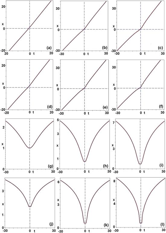
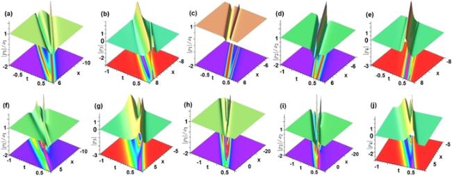
is called the quasi-characteristic curve of the soliton-like propagations in the n-Hirota equation, which is almost a straight line (see figures 1(a), (d) for ${\gamma }_{0}=7,1$). As $\varepsilon =0,\alpha \ne 0$, the corresponding solutions of the n-NLS equation admit the quasi-characteristic curve $x-\mathrm{ln}\sqrt{(m+1)\left[{\left(x+{\gamma }_{0}+1/2\right)}^{2}+{\alpha }^{2}{t}^{2}+1/4\right]/[(n-m)({\gamma }_{0}^{2}+1)]}=0$ which is indeed a curve, not a straight line (see figures 1(g), (j)). Figure 1 implies that the the coefficient ϵ of the third-order dispersive term can change the quasi-characteristic curve for the n-NLS equation into the approximate characteristic straight line for the n-Hirota equation.
In the following, we analyze the asymptotic behaviors of vector semi-rational rogon-soliton solutions (11) by studying the effect of the parameter γ0:
Case 1a.—For the bigger ∣γ0∣, the semi-rational rogon-soliton solutions with non-zero backgrounds pj(x, t)(j = 1, 2,…,m) given by equation (11) can be separated into the rational rogon parts ${p}_{j}^{{rw}}(x,t)(j=1,2,\ldots ,m)$:
whose centers (near t = 0) are localized the domain of x < 0 (see figures 2(a), (c), (d), (f), (g), (i), (j), (k)), and non-travelling-wave grey-like soliton parts with hyperbolic functions ${p}_{j}^{{gs}}(x,t)(j=1,2,\ldots ,m)$:
whose grey parts near t = 0 are localized the domain of x > 0 (see figures 2(a), (c), (d), (f), (g), (i), (j), (k)). Moreover, the semi-rational solitons with zero backgrounds pk(x, t)(k = m + 1,…,n) given by equation (11) tend to the bright-like solitons (see figures 2(b), (e), (h), (l)):
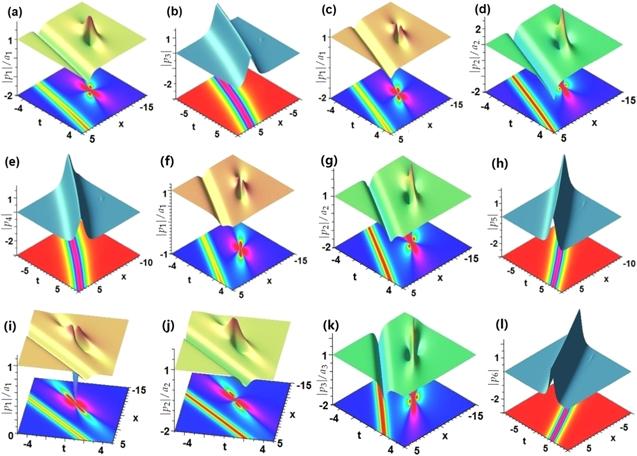
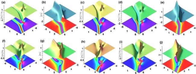
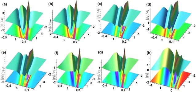
For the bigger value of ∣γ0∣ (e.g. γ0 = 7), figure 2 displays the weak interplays of some types of rational rogons and grey-like solitons, as well as the bright-like solitons and localized tiny waves:
(1)As n = 3, m = 2 corresponding to the 3-Hirota equation with two non-zero backgrounds and one zero background, figure 2(a) displays the semi-rational rogon-soliton solution (∣p1∣/a1) composed of the bright rational rogon ($| {p}_{1}^{{rw}}| /{a}_{1}$) and the grey-like soliton ($| {p}_{1}^{{gs}}| /{a}_{1}$). Figure 2(b) illustrates the bright-like soliton (∣p3∣) made up of the bright soliton ($| {p}_{3}^{{bs}}| )$ and a localized tiny mode;
(2)As n = 4, m = 3 corresponding to the 4-Hirota equation with three non-zero backgrounds and one zero background, figure 2(c) exhibits the semi-rational rogon-soliton (∣p1∣/a1) composed of the four-petaled-shaped rational rogon ($| {p}_{1}^{{rw}}| /{a}_{1}$) and a grey-like soliton ($| {p}_{1}^{{gs}}| /{a}_{1}$). Figure 2(d) illustrates the semi-rational rogon-soliton solution (∣p2∣/a2) consisting of the bright rational rogon ($| {p}_{2}^{{rw}}| /{a}_{2}$) and the grey-like soliton ($| {p}_{2}^{{gs}}| /{a}_{2}$). Figure 2(e) displays the bright-like soliton (∣p4∣) consisting of a bright-like soliton ($| {p}_{4}^{{bs}}| )$ and a localized tiny mode;
(3)As n = 5, m = 4 corresponding to the 5-Hirota equation with four non-zero backgrounds and one zero background, figures 2(f)–(h) exhibit the rogon-soliton (∣p1∣/a1) composed of the four-petaled-shaped rogon ($| {p}_{1}^{{rw}}| /{a}_{1}$) and the grey-like soliton ($| {p}_{1}^{{gs}}| /{a}_{1}$), the semi-rational rogon-soliton solution (∣p2∣/a2) made up of the bright rogon ($| {p}_{2}^{{rw}}| /{a}_{2}$) and the grey-like soliton ($| {p}_{2}^{{gs}}| /{a}_{2}$), and the bright-like soliton (∣p5∣) consisting of the bright soliton ($| {p}_{5}^{{bs}}| $) and a localized tiny mode, respectively;
(4)At n = 6, m = 5 corresponding to the 6-Hirota equation with five non-zero backgrounds and one zero background, figures 2(i)–(l) display the semi-rational rogon-soliton solution (∣p1∣/a1) composed of the dark rogon ($| {p}_{1}^{{rw}}| /{a}_{1}$) and the grey-like soliton ($| {p}_{1}^{{gs}}| /{a}_{1}$), the semi-rational rogon-soliton solution (∣pj∣/aj (j = 2, 3)) made up of the bright rogon ($| {p}_{j}^{{rw}}| /{a}_{j}\,(j=2,3)$) and the grey-like soliton ($| {p}_{j}^{{gs}}| /{a}_{j}\,(j=2,3)$), and the bright-like soliton (∣p6∣) consisting of the bright-like soliton ($| {p}_{6}^{{bs}}| )$ and a localized tiny mode, respectively.
Figure 2. Profiles of weak interactions of rogon-soliton components given by equation (11) with α = 1, ϵ = 0.1, γ0 = 7 for ℓ = 1, n = 3, 4, 5, 6 with m = n − 1. Rogon-soliton components with non-zero backgrounds (a) ∣p1∣/a1 (n = 3), (c), (d) ∣pj∣/aj (j = 1, 2; n = 4), (f), (g) ∣pj∣/aj (j = 1, 2; n = 5), (i)–(k) ∣pj∣/aj (j = 1, 2, 3; n = 6); Soliton-like component with zero backgrounds: (b) ∣p3∣ (n = 3), (e) ∣p4∣ (n = 4), (h) ∣p5∣ (n = 5), (l) ∣p6∣ (n = 6).
The quasi-characteristic curve and velocity.—We find that the non-travelling-wave grey-like solitons ${p}_{j}^{{gs}}(x,t)$ and bright-like solitons ${p}_{k}^{{bs}}(x,t)$ possess the same propagation direction, that is, they all propagate along the approximation curve derived from the quasi-characteristic line (12) in the (x,t)-space
which differs from the propagation direction (the straight line) of usual travelling-wave solitons. Moreover, the same propagation velocity of solitons given by equations (14) and (15) is ${v}_{1}\simeq \tfrac{\varepsilon }{2}{\left(m+1\right)}^{2}\,+\,1/t$, which becomes slow as ∣t∣ increases, and approaches $\tfrac{\varepsilon }{2}{\left(m+1\right)}^{2}$ as ∣t∣ → ∞ .
The time-dependent acceleration.—Now we consider the effect of the bright rogons (13) on the grey-like solitons (14) in these components pj (j = 1,…,m) with non-zero backgrounds for the bigger ∣γ0∣. We study the time-dependent force ${F}_{1}(t)={m}_{1}{{\mathfrak{a}}}_{1}(t)$ on each mass point (e.g. its mass is assumed to be m1) along the quasi-characteristic line (12) arising from the rogons, where the time-dependent acceleration ${{\mathfrak{a}}}_{1}(t)$ of the wave propagations of the grey-like solitons given by equation (14) in the form (see figure 3(a))
where f1(t) = −(α2 + ϵ2)2t2 + ϵ(α2 + ϵ2) (2γ0 + 1) t + (α2 − ϵ2) (${\gamma }_{0}^{2}\,$ + γ0) + α2/2. Figure 3(a) displays the acceleration ${{\mathfrak{a}}}_{1}(t)$ for t ≥ 1. Moreover, ∣a1(t)∣ gradually decreases as t ≥ 1 increases, and approaches zero at t → ∞ . The result implies that the absolute value of the time-dependent force, ∣F1(t)∣, gradually decreases, and approaches zero as t → ∞ .
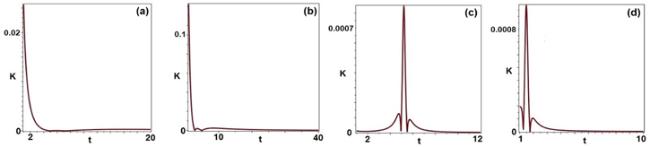
The curvature of the quasi-characteristic curve.—We consider the curvature change of the quasi-characteristic curve (12) or its approximation (16), where the curvature is defined as $K(t)=| {x}^{{\prime\prime} }(t)| /{\left(1+{x}^{{\prime} 2}(t)\right)}^{2},$ from which one has
for the approximate characteristic curve (16). In fact, the corresponding curvature K(t) of the implicit quasi-characteristic curve (12) is so complicated, and not given here, but it can be displayed in figure 4(a) for γ0 = 9, n = 5, m = 4.
Figure 4. The curvatures of the quasi-characteristic curves with γ0 = 9, n = 5, m = 4. (a) α = 1, ϵ = 0.1, ℓ = 1; (b) α = 1, ϵ = 0.1, ℓ = 2; (c) α = 0, ϵ = 2, ℓ = 1; (d) α = 0, ϵ = 2, ℓ = 2.
Acceleration versus distance.—We introduce the distance between the point (x, t) on the quasi-characteristic curve and the center (x0, t0) of the separated rogon as $d:= d(x,t)=\sqrt{{\left(x-{x}_{0}\right)}^{2}+{\left(t-{t}_{0}\right)}^{2}}$, where the center positions of the separated rogons are selected as γ0 = 7$\,\longmapsto \,$(x0, t0) = ( − 7.5, 0), γ0 = 9$\,\longmapsto \,$(x0, t0) = (−9.5, 0). As a result, we give figure 5 to illustrate the relation of the acceleration and distance, which implies that when the distance increases the the absolute value of acceleration decreases, and approaches zero as the distance tends to infinity.
Figure 5. Acceleration versus distance with α = 1, ϵ = 0.1, ℓ = 1. (a) γ0 = 7, n = 3, (b) γ0 = 7, n = 5, (c) γ0 = 9, n = 3, (d) γ0 = 9, n = 5.
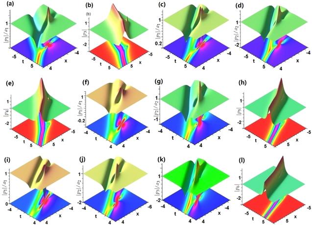
Case 1b.—For the small value of ∣γ0∣ (e.g. γ0 = 1), figure 6 illustrates the strong interplays of different kinds of rational rogons and grey-like solitons, as well as the bright-like solitons and localized bigger waves given by equation (11).
Figure 6. Features of strong interplays of semi-rational rogon-soliton components given by equation (11) with α = 1, ϵ = 0.1, γ0 = 1 for ℓ = 1, n = 3, 4, 5, 6 with m = n − 1. Rogon-soliton components with non-zero backgrounds (a) ∣p1∣/a1 (n = 3), (c), (d) ∣pj∣/aj (j = 1, 2; n = 4), (f), (g) ∣pj∣/aj (j = 1, 2; n = 5), (i)–(k) ∣pj∣/aj (j = 1, 2, 3; n = 6); Soliton-like component with zero backgrounds: (b) ∣p3∣ (n = 3), (e) ∣p4∣ (n = 4), (h) ∣p5∣ (n = 5), (l) ∣p6∣ (n = 6).
Case 2. At ℓ = 2, we take γ1 = 0.5i, γ2 = 1, γj+1 = 0 (ℓ = 2, 3, 4), and ri,j = 1(j = 0, 1, 2) to find the vector semi-rational rogon-soliton and soliton-like solutions with a free real parameter γ0 of the n-Hirota equation
which is almost a straight line (see figures 1(b), (e)) except for the tiny bend near the point $(0,0)$. However when $\varepsilon =0,\alpha =1$, the corresponding quasi-characteristic curves of the n-NLS equation are displayed in figures 1(h), (k).
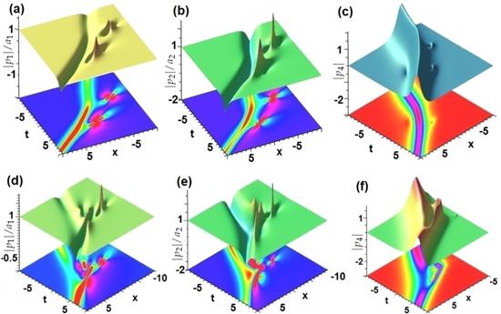
Case 2a.—For the bigger value of ∣γ0∣, we consider the asymptotic analysis to decompose the obtained vector semi-rational rogon-soliton solutions (19). The semi-rational rogon-soliton solutions pj(x, t)(j = 1, 2,…,m) given by equation (11) can be decomposed into the rational rogon parts ${p}_{j}^{{rw}}(x,t)$
whose grey parts near t = 0 are localized the domain of x > 0 (see figure 7). Moreover, the semi-rational soliton ps(x, t)(s = m + 1,…,n) given by equation (19) approaches to a bright-like soliton
For the bigger value of ∣γ0∣ (e.g. γ0 = 8), figure 7 displays the structures of weak interplays of different kinds of rational rogons and grey-like solitons, as well as the bright-like solitons and localized tiny waves given by equation (19): (1) At n = 3, m = 2, figures 7(a), (b) illustrate the weak interplay (∣p1∣/a1) made up of the two-bright rational rogon ($| {p}_{1}^{{rw}}| /{a}_{1}$) and grey-like soliton ($| {p}_{1}^{{gs}}| /{a}_{1}$), and the bright-like soliton (∣p3∣) consisting of the bright-like soliton ($| {p}_{3}^{{bs}}| )$ and a localized tiny mode with one hump and one dip, respectively; (2) As n = 4, m = 3, figures 7(c)–(e) exhibit the features of ∣p1∣/a1 composed of the two-four-petaled-shaped rogon ($| {p}_{1}^{{rw}}| /{a}_{1}$) and grey-like soliton ($| {p}_{1}^{{gs}}| /{a}_{1}$), the ∣p2∣/a2 consisting of two-bright rogon ($| {p}_{2}^{{rw}}| /{a}_{2}$) and grey-like soliton ($| {p}_{2}^{{gs}}| /{a}_{2}$),and bright-like soliton (∣p4∣) consisting of the bright-like soliton ($| {p}_{4}^{{bs}}| )$ and a localized tiny mode with one hump and one dip, respectively. Equations (22) and (23) imply that the grey-like solitons ${p}_{j}^{{gs}}(x,t)$ and bright-like solitons ${p}_{k}^{{bs}}(x,t)$ have the same propagation direction along the approximation curve derived from the quasi-characteristic curve (20)
which differs from the propagation direction (the straight line) of usual travelling-wave solitons. Moreover, the same propagation velocity of solitons given by equations (22) and (23) is ${v}_{2}\simeq \tfrac{\varepsilon }{2}{\left(m+1\right)}^{2}+2/t$, which becomes slow as ∣t∣ increases, and approaches $\tfrac{\varepsilon }{2}{\left(m+1\right)}^{2}$ as ∣t∣ → ∞ . Similarly to ℓ = 1, we can also consider the time-dependent accelerations for ℓ = 2 (see figure 3(b)). The corresponding curvature of the quasi-characteristic line is exhibited in figure 4(b) for γ0 = 9, n = 5, m = 4.
Figure 7. Profiles of weak and strong interactions of rogon-soliton given by equation (19) with α = 1, ϵ = 0.1 and ℓ = 2, n = 3, 4, m = n − 1. Weak interactions with γ0 = 8: Non-zero backgrounds (a) ∣p1∣/a1 (n = 3), (c), (d) ∣pj∣/aj (j = 1, 2; n = 4); Soliton-like components with zero background: (b) ∣p3∣ (n = 3), (e) ∣p4∣ (n = 4). Strong interactions with γ0 = −0.5: Non-zero backgrounds (f) ∣p1∣/a1 (n = 3), (h), (i) ∣pj∣/aj (j = 1, 2; n = 4), and soliton-like components with zero backgrounds: (g) ∣p3∣ (n = 3), (j) ∣p4∣ (n = 4).
Case 2b.—For the smaller value of ∣γ0∣ (e.g. γ0 = − 0.5), figures 7(f)–(j) exhibit the features of strong interactions of different kinds of two-rogons and grey-like solitons, as well as bright-like solitons and localized tiny modes given by equation (19).
Case 3. As ℓ = 3, i.e. γ0γ1γ2γ3 ≠ 0, γj+1 = 0 (j = 3, 4,…,n), and ri,j = 1(j = 0, 1, 2, 3). We take γ1 = 0.5i, γ2 = 1, γ3 = i to find the semi-rational vector rogon-soliton and soliton-like solutions (8) of the n-Hirota equation (2)
which is almost a straight line (see figures 1(c), (f)) except for the tiny bend near the point $(0,0)$. However when $\varepsilon =0,\alpha =1$, the corresponding quasi-characteristic curves of the n-NLS equation are displayed in figures 1(i), (l).
In the following, we analyze the asymptotic behaviors of vector semi-rational rogon-soliton solutions (25) by studying the effect of the parameter γ0:
Case 3a.—For the bigger ∣γ0∣, we consider the asymptotic analysis to decompose the obtained vector semi-rational rogon-soliton solutions (25). The semi-rational rogon-soliton solutions pj(x, t)(j = 1, 2,…,m) given by equation (25) can be decomposed into the rational rogon parts ${p}_{j}^{{rw}}(x,t)$
whose grey-like parts near t = 0 are localized the domain of x > 0 (see figure 7). Moreover, the semi-rational soliton pk(x, t)(k = m + 1,…,n) given by equation (25) approaches to a bright-like soliton
Figure 8. Features of weak and strong interplays for the semi-rational rogon-soliton components with non-zero boundary conditions given by equation (25) with α = 1, ϵ = 0.1 and ℓ = 3, n = 4, m = n − 1. Weak interactions with γ0 = 15: (a), (b) ∣pj∣/aj (j = 1, 2; n = 4), and soliton-like component with zero backgrounds: (c) ∣p3∣ (n = 3). Weak interactions with γ0 = −0.5: (d), (e) ∣pj∣/aj (j = 1, 2; n = 4), and soliton-like component with zero backgrounds: (f) ∣p4∣ (n = 4).
It follows from equations (28) and (29) that the grey-like solitons ${p}_{j}^{{gs}}(x,t)$ and bright-like solitons ${p}_{k}^{{bs}}(x,t)$ have the same propagation direction along the approximation curve derived from the quasi-characteristic line (26)
where f is a polynomial of x, t. The direction given by equation (30) differs from the propagation direction (the straight line) of usual travelling-wave solitons. Moreover, the same propagation velocity of solitons given by equations (28) and (29) is ${v}_{3}\simeq \tfrac{\varepsilon }{2}{\left(m+1\right)}^{2}\,+\,3/t$, which becomes slow as ∣t∣ increases, and approaches $\tfrac{\varepsilon }{2}{\left(m+1\right)}^{2}$ as ∣t∣ → ∞ . Similarly to ℓ = 1, 2, we can also consider the time-dependent accelerations for ℓ = 3 (see figure 3(c)).
Case 3b.—For the smaller value of ∣γ0∣ (e.g. γ0 = −0.5), figures 8(d)–(f) exhibit the strong interactions of different kinds of two-rogons and grey-like solitons, as well as bright-like solitons and localized tiny waves given by equation (25).
4. Semi-rational rogon-soliton solutions with ultra-high amplitudes
In this section, we will consider the maximal amplitudes of the vector semi-rational rogon-soliton solutions given by equation (8). We will consider two the average amplitudes as follows:
where ${\boldsymbol{p}}(x,t)={\left({p}_{1},{p}_{2},\ldots ,{p}_{n}\right)}^{{\rm{T}}}$, ${\boldsymbol{a}}={\left({a}_{1},{a}_{2},\ldots ,{a}_{n}\right)}^{{\rm{T}}}$ with aj ≠ 0 (j = 1, 2,…,m).
For the given the vector semi-rational rogon-soliton solutions (8), ${{ \mathcal A }}_{{all}},{{ \mathcal A }}_{e,j}$ can be attained at $\{{\boldsymbol{c}}={\left(\sqrt{n},{\rm{i}},\ldots ,{\rm{i}}\right)}^{{\rm{T}}}$, (x, t) = (0, 0)} and $\{{\boldsymbol{c}}={\left(\mathrm{1,0},\ldots ,0,{\rm{i}},0,\ldots ,0\right)}^{{\rm{T}}}$, $(x,t)=(0,0)\}$ (non-zero number ${\rm{i}}$ in the ${\boldsymbol{c}}$ is the $(j+1)$-th entry), respectively, in the forms
$\begin{eqnarray}\begin{array}{l}{{ \mathcal A }}_{{all}}=1+\displaystyle \frac{(m+1)\sqrt{n}}{{\sum }_{j=1}^{m}\csc {w}_{j}}={ \mathcal O }\left(\displaystyle \frac{\sqrt{n}}{\mathrm{ln}m}\right),\\ {{ \mathcal A }}_{e,j}=1+(m+1)\sin {w}_{j},\\ {w}_{j}=\displaystyle \frac{j\pi }{m\,+\,1},\quad j\,=\,1,\ldots ,m.\end{array}\end{eqnarray}$
Firstly, we should note that ${{ \mathcal W }}_{(n+1)\times (n+1)}(0,0)$ given by equation (9) is
Given the (n+1)-dimensional vectors ${\mathfrak{W}}={\left(| {\alpha }_{0}| ,| {\alpha }_{1}| {\rm{i}},\ldots ,| {\alpha }_{n}| {\rm{i}}\right)}^{{\rm{T}}}$, ${ \mathcal W }{\boldsymbol{c}}={\left({\alpha }_{0},{\alpha }_{1},\ldots ,{\alpha }_{n}\right)}^{{\rm{T}}}$, and ${\beta }_{j}=| {\alpha }_{j}| $, we have
$\begin{eqnarray}\begin{array}{l}\displaystyle \frac{{\sum }_{j=1}^{n}\left|{a}_{j}-2{\rm{i}}(m+1)\tfrac{{{ \mathcal W }}_{j+1}{\boldsymbol{c}}{\left({{ \mathcal W }}_{1}{\boldsymbol{c}}\right)}^{* }}{{\left({ \mathcal W }{\boldsymbol{c}}\right)}^{\dagger }({ \mathcal W }{\boldsymbol{c}})}\right|}{{\sum }_{j=1}^{m}\csc {w}_{j}}\\ ={\sum }_{j=1}^{n}\left|\displaystyle \frac{{a}_{j}}{{\sum }_{j=1}^{m}\csc {w}_{j}}-2{\rm{i}}(m+1)\displaystyle \frac{{{ \mathcal W }}_{j+1}{\boldsymbol{c}}{\left({{ \mathcal W }}_{1}{\boldsymbol{c}}\right)}^{* }}{{{\mathfrak{W}}}^{\dagger }{\mathfrak{W}}{\sum }_{j\,=\,1}^{m}\csc {w}_{j}}\right|\\ \leqslant {\sum }_{j=1}^{n}\left|\displaystyle \frac{{a}_{j}}{{\sum }_{j=1}^{m}\csc {w}_{j}}+\displaystyle \frac{2(m+1){\beta }_{j}{\beta }_{0}}{\left({\sum }_{j=0}^{n}{\beta }_{j}^{2})({\sum }_{j=1}^{m}\csc {w}_{j}\right)}\right|\\ \leqslant 1+\displaystyle \frac{(m+1)\sqrt{n}}{{\sum }_{j=1}^{m}\csc {w}_{j}}.\end{array}\end{eqnarray}$
The last equality holds if and only if ${\beta }_{0}=\sqrt{n}{\beta }_{i},{\beta }_{i}\,={\beta }_{j},0\lt i,j\leqslant n$. According to (35), we have the expression of ${{ \mathcal A }}_{{all}}$ in equation (33). Notice that since ${ \mathcal W }(x,t)$ is a unit matrix at $(0,0)$, so we can take ${\boldsymbol{c}}={\left(\sqrt{n},{\rm{i}},\ldots ,{\rm{i}}\right)}^{{\rm{T}}}$. In the same way, according to
we have the expression of ${{ \mathcal A }}_{e,j}$ in equation (33). Notice that ${ \mathcal W }(0,0)={{\mathbb{I}}}_{n+1}$, thus one can take ${\boldsymbol{c}}={\left(\mathrm{1,0},\ldots ,0,{\rm{i}},0,\ldots ,0\right)}^{{\rm{T}}}$. This completes the proof.
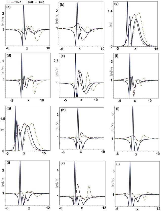
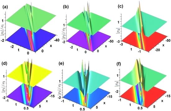
In particular, we display the profiles of the 3-Hirota and 4-Hirota equations when Tall and Te,j are attained for at $\{{\boldsymbol{c}}\,={\left(\sqrt{n},{\rm{i}},\ldots ,{\rm{i}}\right)}^{{\rm{T}}}$, (x, t) = (0, 0)} and $\{{\boldsymbol{c}}={\left(\mathrm{1,0},\ldots ,0,{\rm{i}},0,\ldots ,0\right)}^{{\rm{T}}}$, (x, t) = (0, 0)}, respectively (see figure 9).
Figure 9. Profiles of the semi-rational rogon-soliton solutions given by equation (8) with α = 1, ε = 0.1. The case of ${{ \mathcal A }}_{{all}}$: (a)–(c) $n=3,m=2,{c}_{0}=\sqrt{3},{c}_{\mathrm{1,2,3}}={\rm{i}};$ (d)–(g) n = 4, m = 3, c0 = 2, c1,2,3,4 = i; The case of ${{ \mathcal A }}_{e,j}$: (i) n = 3, m = 2: (h) ∣p1∣/a1, c0 = 1, c1 = i, cj = 0(j = 2, 3), (i) ∣p2∣/a2, c0 = 1, c2 = i, cj = 0(j = 1, 3); (ii) n = 4, m = 3: (j) ∣p1∣/a1, c0 = 1, c1 = i, cj = 0(j = 2, 3, 4), (k) ∣p2∣/a2, c0 = 1, c2 = i, cj = 0(j = 1, 3, 4), (l) ∣p3∣/a3, c0 = 1, c3 = i, cj = 0(j = 1, 2, 4).
5. Vector semi-rational solitons of the n-cmKdV equation
At α = 0, ϵ ≠ 0, we can find the vector semi-rational solitons of the n-cmKdV equation (3) from the solutions (8), where ${\zeta }_{1}=x-\tfrac{3}{2}\varepsilon t(1+\parallel {\boldsymbol{a}}{\parallel }^{2}),{\zeta }_{2}=\tfrac{3{\rm{i}}}{2}\varepsilon t,{\zeta }_{3}=\tfrac{1}{2}\varepsilon t.$ Notice that the separated rational solutions are solitons, not rogons, which mainly result from ${\zeta }_{1}=x-\tfrac{3}{2}\varepsilon t(1+\parallel {\boldsymbol{a}}{\parallel }^{2})$ is a real-valued linear function of x, t, and ${\zeta }_{2}=\tfrac{3{\rm{i}}}{2}\varepsilon t$ is a pure imaginary function of t, however, ${\zeta }_{1}=x+{\rm{i}}\alpha t-\tfrac{3}{2}\varepsilon (1+\parallel {\boldsymbol{a}}{\parallel }^{2})t$ is a complex-valued linear function of x, t, and ${\zeta }_{2}=\tfrac{3{\rm{i}}}{2}\varepsilon t+\tfrac{1}{2}\alpha t$ is also a complex-valued function of t for the n-Hirota equation with αϵ ≠ 0.
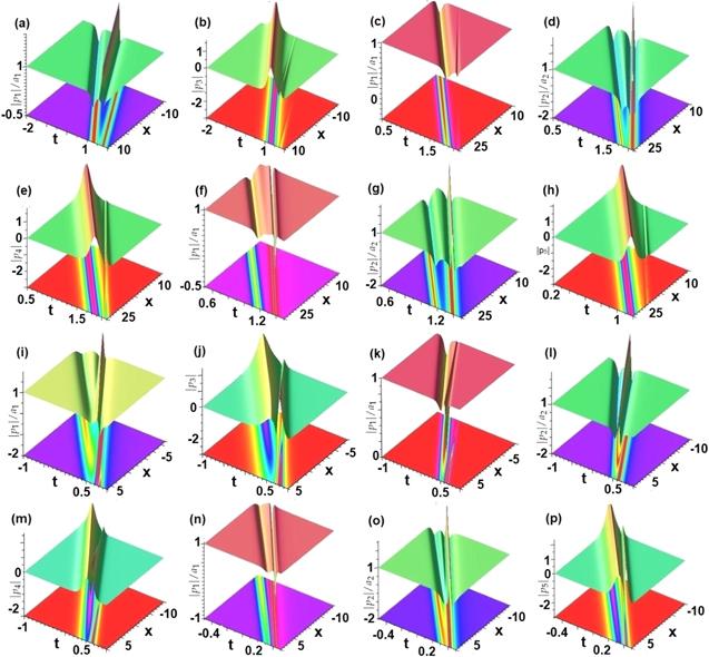
Case 1. For the ℓ = 1, we have the vector semi-rational solitons of the n-cmKdV equation (3) in the form (11) with α = 0. Figures 10(a)–(h) display the weak interactions for the larger γ0 = 7 and n = 3, 4, 5 with m = n − 1, and the strong interactions are illustrated in figures 10(i)–(p) for the smaller γ0 = 1 and n = 3, 4, 5 with m = n − 1.
Figure 10. Profiles of the semi-rational solitons (11) with α = 0, ϵ = 2 for ℓ = 1, n = 3, 4, 5 with m = n − 1. Weak interactions with γ0 = 7: grey-like and W-shaped solitons with non-zero backgrounds (a) ∣p1∣/a1 (n = 3), (c), (d) ∣pj∣/aj (j = 1, 2; n = 4), (f), (g) ∣pj∣/aj (j = 1, 2; n = 5), and soliton-like components with zero backgrounds: (b) ∣p3∣ (n = 3), (e) ∣p4∣ (n = 4), (h) ∣p5∣ (n = 5). Strong interactions with γ0 = 1 for n = 3, 4, 5 with m = n − 1: grey-like and W-shaped solitons with non-zero backgrounds (i) ∣p1∣/a1 (n = 3), (k), (l) ∣pj∣/aj (j = 1, 2; n = 4), (o, p) ∣pj∣/aj (j = 1, 2; n = 5), and soliton-like component with zero backgrounds: (j) ∣p3∣ (n = 3), (m) ∣p4∣ (n = 4), (p) ∣p5∣ (n = 5).
Similarly to the n-Hirota equation, we can also consider the time-dependent accelerations in the n-cmKdV equation for ℓ = 1 (see figure 3(d)). The corresponding curvature of the quasi-characteristic line is exhibited in figure 4(c) for γ0 = 9, n = 5, m = 4.
Case 2. For ℓ = 2, we find the vector semi-rational solitons of the n-cmKdV equation (3) in the form (19) with α = 0. Figures 11(a)–(e) display the weak interactions for the larger γ0 = 8 and n=3,4 with m = n − 1, and the strong interactions are illustrated in figures 11(f)–(j) for the smaller γ0 = − 0.5 and n = 3, 4 with m = n − 1.
Figure 11. Profiles of weak interactions for the semi-rational rogon-soliton components with non-zero backgrounds given by equation (19) with α = 0, ϵ = 2, γ0 = 8 for ℓ = 2, n = 3, 4 with m = n − 1: (a) ∣p1∣/a1 (n = 3), (c), (d) ∣pj∣/aj (j = 1, 2; n = 4), and soliton-like component with zero backgrounds: (b) ∣p3∣ (n = 3), (e) ∣p4∣ (n = 4). Strong interactions with α = 0, ϵ = 2, γ0 = −0.5 for ℓ = 2, n = 3, 4 with m = n − 1: (f) ∣p1∣/a1 (n = 3), (h), (i) ∣pj∣/aj (j = 1, 2; n = 4), and soliton-like component with zero backgrounds: (g) ∣p3∣ (n = 3), (j) ∣p4∣ (n = 4).
Similarly to the n-Hirota equation, we can also consider the time-dependent accelerations in the n-cmKdV equation for ℓ = 2 (see figure 3(e)). The corresponding curvature of the quasi-characteristic line is exhibited in figure 4(d) for γ0 = 9, n = 5, m = 4.
Case 3. As ℓ = 3, we find the vector semi-rational solitons of the n-cmKdV equation (3) in the form (25) with α = 0. Figures 12(a)–(c) display the weak interactions for the larger γ0 = 15 and n = 4, m = 3, and the strong interactions are illustrated in figures 12(d)–(f) for the smaller γ0 = − 0.5 and n = 4, m = 3. Similarly to the n-Hirota equation, we can also consider the time-dependent accelerations for ℓ = 3 (see figure 3(f)).
Figure 12. Profiles of weak interactions for the semi-rational rogon-soliton components with non-zero backgrounds given by equation (25) with α = 0, ϵ = 2, γ0 = 15 for ℓ = 3, n = 4 with m = n − 1: (a), (b) ∣pj∣/aj (j = 1, 2; n = 4), and soliton-like component with zero backgrounds: (c) ∣p3∣ (n = 3). Strong interactions with α = 0, ϵ = 2, γ0 = −0.5 for ℓ = 3, n = 4 with m = n − 1: (d), (e) ∣pj∣/aj (j = 1, 2; n = 4), and soliton-like component with zero backgrounds: (f) ∣p4∣ (n = 4).
Similarly, the results in section 4 with α = 0, ϵ ≠ 0 also hold for the n-cmKdV equation (3), which are displayed in figure 13 for some parameters.
Figure 13. Profiles of the semi-rational soliton solutions given by equation (8) with α = 0, ε = 2. The case of ${{ \mathcal A }}_{e,j}$: (i) n = 3, m = 2 (a) ∣p1∣/a1, c0 = 1, c1 = i, cj = 0(j = 2, 3), (b) ∣p2∣/a2, c0 = 1, c2 = i, cj = 0(j = 1, 3); (ii) n = 4, m = 3: (c) ∣p1∣/a1, c0 = 1, c1 = i, cj = 0(j = 2, 3, 4), (d) ∣p2∣/a2, c0 = 1, c2 = i, cj = 0(j = 1, 3, 4), (e) ∣p3∣/a3, c0 = 1, c3 = i, cj = 0(j = 1, 2, 4). The case of ${{ \mathcal A }}_{{all}}$: (f)–(h) $n=3,m=2,{c}_{0}=\sqrt{3},{c}_{\mathrm{1,2,3}}={\rm{i}}$.
6. Conclusions and discussions
In conclusion, we start with the mixed background seed solutions and obtain the semi-rational rogon-soliton solutions of the n-Hirota equation through the modified Darboux transformation. Firstly, we require the selection of parameters makes the characteristic polynomial admit the (m + 1)-multiple root and (n − m) simple roots, and then it is brought into the modified Darboux transform to find the semi-rational solutions of the n-Hirota equation. Finally, the exact semi-rational solutions of the n-Hirota equation are analyzed in detail for the cases of ℓ = 1, 2, 3 and n = 3, 4, 5, 6. The semi-rational rogon-soliton solutions of first m components with non-zero backgrounds can be decomposed into the rational rogon solutions and the grey-like solitons. The last (n − m) components with zero backgrounds are gradually decayed to the bright-like solitons. The interactions between rogons and soliton-like solutions are characterized by analyzing the accelerations and curvatures along the quasi-characteristic curves. We also study the semi-rational solitons of the n-cmKdV equation. The ideas and methods used in this paper can be extended to other nonlinear integrable physical models. Among them, the higher-order Darboux transformation of n-Hirota equation can also be studied in future.
This work was supported by the National Natural Science Foundation of China (Nos. 11 925 108 and 11 731 014).
PengWPuJChenY2022 PINN deep learning method for the Chen-Lee-Liu equation: Rogue wave on the periodic background Commun. Nonlinear Sci. Numer. Simul.105 106067
ZakharovV EShabatA B1972 Exact theory of two-dimensional self-focusing and one-dimensional self-modulation of waves in nonlinear media Sov. Phys. JETP34 62
23
HirotaR1973 Exact envelope-soliton solutions of a nonlinear wave equation J. Math. Phys.14 805
YangYWangXYanZ2015 Optical temporal rogue waves in the generalized inhomogeneous nonlinear Schrödinger equation with varying higher-order even and odd terms Nonlinear Dyn.81 833
WengWYanZ2021 Inverse scattering and N-triple-pole soliton and breather solutions of the focusing nonlinear Schrödinger hierarchy with nonzero boundary conditions Phys. Lett. A407 127472
ZhangGYanZWenXChenY2017 Interactions of localized wave structures and dynamics in the defocusing coupled nonlinear Schrödinger equations Phys. Rev. E95 042201
ZhangGYanZWangL2019 The general coupled Hirota equations: modulational instability and higher-order vector rogue wave and multi-dark soliton structures Proc. R. Soc. A475 20180625
WengWZhangGZhouZYanZ2022 Semi-rational vector rogon-soliton solutions of the five-component Manakov/NLS system with mixed backgrounds Appl. Math. Lett.125 107735


