


1. Introduction
Although mature paradigms, like the celebrated Fermi liquid theory [1–3] and Luttinger liquid theory [4, 5], enable us to understand well a wide class of many-body systems in the stationary state, their dynamical evolution is much less understood. In fact, quantum dynamics of many-body systems always presents itself with formidable challenges, due to the difficulty of deriving eigenfunctions analytically and the exponentially growing complexity of numerics. Despite these theoretical difficulties, significant progresses have been made in the last decade, which greatly improves our understanding of dynamical properties of many-body systems. For example, the Kibble–Zurek mechanism [6] reveals power-law relations between the typical length scale ξ of defect domains, the relaxation time τ, and the rate of change of the driving parameter λ, namely ξ ∼ λ−ν and τ ∼ λ−zν, which has been observed in ion Coulomb crystals [7]. Thermalization of isolated many-body systems is also a difficult topic. The eigenstate thermalization hypothesis (ETH) [8, 9] asserts that, for a closed systems evolving to the steady state, the diagonal and micro-canonical ensembles are equivalent. In recent experiments with ultracold atoms [10, 11], Kinoshita et al showed that Bose gases in one-dimensional traps do not thermalize, even after thousands of collisions [12]. The ETH can be violated by integrable models [13], due to the existence of infinitely many conserved charges, or in the presence of many-body localization [14]. The study of dynamics is of crucial importance for many-body quantum systems out of equilibrium, as it provides important clues on if and how their equilibrium state can be reached.
Therefore, while thermalization usually concerns the steady-state properties of many-body systems after a long-time evolution, an interesting question is on how the many-body system evolves at intermediate times. For a system with a short-range interaction, like the Heisenberg spin chain and the Lieb–Lininger model, light-cone dynamics dominates the relaxation of local observables to steady-state values, such as spin polarization and correlation functions [15]. However, the relaxation process of local and global quantities to the steady state is less explored in models with long-range interactions. In this paper, we use Gaudin magnets, i.e. the inhomogeneous central spin models, to study the relaxation dynamics of many-body systems. Such magnets with long-range interactions may describe the decoherence of a spin-qubit due to the interaction with surrounding spins, for example an electron interacting with nuclear spins in quantum dots or defect centers [16, 17]. Quantum dynamics of the Gaudin model has been extensively studied with a variety of methods as, for example, exact diagonalization and quantum many-body expansions [17–22], the Bethe ansatz method for the polarized bath with one flipped bath spin [23], hybrid methods combining the Bethe ansatz and Monte Carlo sampling [24, 25], the DMRG method and semiclassical approaches [26–29].
While an early description of Gaudin magnets using the Bethe ansatz technique considered one flipped bath spin, i.e. M = 1 [23], here we study the time evolution of the central spin problem with an arbitrary number of flipped spins M, starting from an initial state $| {{\rm{\Phi }}}_{0}\rangle ={s}_{{a}_{1}}^{-}\cdots {s}_{{a}_{M}}^{-}| \Uparrow \rangle =| {a}_{1},\cdots ,{a}_{M}\rangle $ , where ∣ ⇑ ⟩ is the fully polarized state and ai = 0, 1, 2, ...N label the positions of spins in the system. The quantum dynamics of the model with arbitrary number of flipped spins has been already studied through Bethe ansatz [24, 25], as well as various other theoretical approaches, leading to important insights such as a description of quantum decoherence by the Chebyshev expansion method [33], non-Markovian dynamics [20], persistent spin correlations [34], etc. Here we study the time evolutions of several interesting quantities analytically and numerically: the spin distribution function, the spin–spin correlation function, and the Loschmidt echo. Evaluating these, we find that the time dependence of the spin polarization function reveals a breakdown of thermalization, such that the steady-state of the Gaudin magnets cannot be described by an equilibrium ensemble. Instead, the relaxation to steady-state values of the spin–spin correlation function suggests a logarithmic decay, and we find that at intermediate times the Loschmidt echo relaxes exponentially to its steady-state value, using both the Bethe ansatz solution and matrix product states (MPS) numerical approach.
2. Model and Bethe ansatz equations
The Gaudin magnet describes a central spin at position ‘0' coupled to bath spins through long-range interactions. The Hamiltonian reads${H}_{j}=B{{\boldsymbol{s}}}_{j}^{z}+{\sum }_{k\ne j}{{\boldsymbol{s}}}_{j}\cdot {{\boldsymbol{s}}}_{k}/({\epsilon }_{j}-{\epsilon }_{k})$ [35–37]. Following the algebraic Bethe ansatz method, and considering a subspace where M spins are flipped-down with respect to the reference state ∣ ⇑ ⟩, the eigenstates are given below [35, 36]:3 ) are also called Richardson–Gaudin equations. There are ${C}_{N+1}^{M}$ sets of solutions to equation (3 ), which correspond to the number of choices of flipping M spins [38]. These ${C}_{N+1}^{M}$ states ∣ν1, ⋯ ,νM⟩ span the subspace with M spins flipped-down. In appendix D we give details of the numerical method for solving the Bethe Ansatz equation (3 ). Moreover, their eigenenergy is given by
$\begin{eqnarray}H=B{{\boldsymbol{s}}}_{0}^{z}+2\sum _{j=1}^{N}{A}_{j}{{\boldsymbol{s}}}_{0}\cdot {{\boldsymbol{s}}}_{j},\end{eqnarray}$
where the bath spins are labelled with 1 → N. For convenience, we parametrize the magnetic field as B = −2/g. Furthermore, we write Aj = 1/(ε0 − εj) for the inhomogeneous interaction strength determined in experiments. Setting ε0 = 0, the εj (with j = 1, …, N) correspond to the energy levels of a discrete BCS model associated with H, which can be constructed from the conserved quantities $\begin{eqnarray}| {\nu }_{1},\cdots ,{\nu }_{M}\rangle =\prod _{\alpha =1}^{M}{B}_{{\nu }_{\alpha }}| \Uparrow \rangle =\prod _{\alpha =1}^{M}\sum _{j=0}^{N}\displaystyle \frac{{s}_{j}^{-}}{{\nu }_{\alpha }-{\epsilon }_{j}}| \Uparrow \rangle ,\end{eqnarray}$
where the M parameters {να} should satisfy the following Bethe ansatz equations $\begin{eqnarray}\sum _{j=0}^{N}\displaystyle \frac{1}{{\nu }_{\alpha }-{\epsilon }_{j}}=\displaystyle \frac{2}{g}+\sum _{\beta \ne \alpha ,\beta =1}^{M}\displaystyle \frac{2}{{\nu }_{\alpha }-{\nu }_{\beta }},\end{eqnarray}$
with α = 1, 2, …, M. The equation ( $\begin{eqnarray}E=\displaystyle \frac{B}{2}+\displaystyle \frac{1}{2}\sum _{j=1}^{N}\displaystyle \frac{1}{{\epsilon }_{0}-{\epsilon }_{j}}-\sum _{\alpha =1}^{M}\displaystyle \frac{1}{{\epsilon }_{0}-{\nu }_{\alpha }}.\end{eqnarray}$
We exploited the above eigenfunctions to study the quantum dynamics of the central spin model. The initial state (see introduction) is a simple product state ∣Φ0⟩ = ∣a1, ⋯ , aM⟩, where {a1, ⋯ , aM} is a set of mutually unequal site indexes which can range from ‘0' to ‘N'. After the interaction is switched on, the wave function evolves as$| {\phi }_{k}\rangle ={N}_{{\nu }_{k}}| {\nu }_{1,k},\cdots ,{\nu }_{M,k}\rangle $ , with ${N}_{{\nu }_{k}}$ the normalization coefficient7(7See the appendix for details. There we present brief derivations for the time evolution of the spin distribution function, the spin–spin correlation function, and the Loschmidt echo for the Gaudin magnet with arbitrary number of flipped spins M.)(see appendix B ). The index ‘k' labels all the states corresponding to the roots of equation (3 ). Since the initial state has M spins which are flipped-down, we only need to consider the Bethe ansatz basis in this particular subspace. A critical quantity in equation (5 ) is the overlap between the initial state and the eigenfunctions, given as follows:${ \mathcal P }$ ' means summing over all permutation of indexes {a1, ⋯ , aM}, see appendices A and B . The overlap can be also written as $\langle {{\rm{\Phi }}}_{0}| {\phi }_{k}\rangle ={N}_{{\nu }_{k}}\ \mathrm{perm}(1/({\nu }_{\alpha ,k}-{\epsilon }_{{{ \mathcal P }}_{\alpha }}))$ , where ‘perm' is the permanent of matrix $1/({\nu }_{\alpha ,k}-{\epsilon }_{{{ \mathcal P }}_{\alpha }})$ , similar to the determinant [35, 36]. It is worth noting that both permanent and determinant representation can give the exact quantum dynamics of the Gaudin magnets. However, the numerical tasks from the two representations is quite different as determinants can be evaluated in polynomial time. The interested readers can find more details about permanent and determinant representations in [39–41]. For either representation, it still remains challenging to get dynamical quantities for the Gaudin magnets with a large system size, and values up to N = 48 were reached [24].
$\begin{eqnarray}| \psi (t)\rangle =\sum _{k}| {\phi }_{k}\rangle \langle {\phi }_{k}| {{\rm{\Phi }}}_{0}\rangle {{\rm{e}}}^{-{\rm{i}}{E}_{k}t},\end{eqnarray}$
where we introduced the orthonormalized wave functions $\begin{eqnarray}\langle {{\rm{\Phi }}}_{0}| {\phi }_{k}\rangle ={N}_{{\nu }_{k}}\sum _{{ \mathcal P }\in \{{a}_{1},\cdots ,{a}_{M}\}}\prod _{\alpha =1}^{M}\displaystyle \frac{1}{({\nu }_{\alpha ,k}-{\epsilon }_{{{ \mathcal P }}_{\alpha }})},\end{eqnarray}$
where ‘From expressions (5 ) and (6 ), the evolution of observables (for example the spin distribution) can be calculated rather straightforwardly. Based on this approach, we will present in the rest of the paper our key analytical and numerical results on the quantum dynamics of Gaudin magnets.
3. Spin distribution
By making use of equation (5 ), the time-dependent polarization of site j is immediately written as${w}_{{{kk}}^{{\prime} }}={E}_{{k}^{{\prime} }}-{E}_{k}$ simplifies to ${\sum }_{\alpha =1}^{M}1/({\epsilon }_{0}-{\nu }_{\alpha ,k})\,-{\sum }_{\alpha =1}^{M}1/({\epsilon }_{0}-{\nu }_{\alpha ,{k}^{{\prime} }})$ . While the overlaps are given in equation (6 ), the remaining difficulty is to obtain the matrix elements of the observable in the eigenfunction basis. As detailed in appendix B , one can insert the complete set of states ∣a1, ⋯ , aM⟩, thus writing the matrix elements in terms of overlaps of type ⟨Φ0∣φk⟩. We finally obtain the exact expression:${ \mathcal P }$ ' and ‘${ \mathcal Q }$ ' indicate summing over all the permutations of indexes {a1, ⋯ , aM} and {j1, ⋯ , jM}, respectively.
$\begin{eqnarray}\displaystyle {s}_{j}^{z}(t)=\sum _{k}\sum _{{k}^{{\prime} }}\langle {{\rm{\Phi }}}_{0}| {\phi }_{k}\rangle \langle {\phi }_{k}| {s}_{j}^{z}| {\phi }_{{k}^{{\prime} }}\rangle \langle {\phi }_{{k}^{{\prime} }}| {{\rm{\Phi }}}_{0}\rangle {{\rm{e}}}^{-{\rm{i}}{w}_{{{kk}}^{{\prime} }}t},\end{eqnarray}$
where $\begin{eqnarray}\displaystyle \begin{array}{l}{s}_{j}^{z}(t)=\displaystyle \frac{1}{2}-\sum _{k}\sum _{{k}^{{\prime} }}\cos ({w}_{{{kk}}^{{\prime} }}t)\sum _{{j}_{1}\lt \cdots \lt {j}_{M}}\sum _{\alpha =1}^{M}{\delta }_{{{jj}}_{\alpha }}\\ \quad \times \sum _{{ \mathcal P }}\sum _{{ \mathcal Q }}\displaystyle \frac{| {N}_{{\nu }_{k}}{| }^{2}}{\prod _{\alpha =1}^{M}({\nu }_{\alpha ,k}-{\epsilon }_{{{ \mathcal P }}_{\alpha }})({\nu }_{\alpha ,k}-{\epsilon }_{{{ \mathcal Q }}_{\alpha }})}\\ \quad \times \sum _{{ \mathcal P }}\sum _{{ \mathcal Q }}\displaystyle \frac{| {N}_{{\nu }_{k^{\prime} }}{| }^{2}}{\prod _{\alpha =1}^{M}({\nu }_{\alpha ,k^{\prime} }-{\epsilon }_{{{ \mathcal P }}_{\alpha }})({\nu }_{\alpha ,k^{\prime} }-{\epsilon }_{{{ \mathcal Q }}_{\alpha }})},\end{array}\end{eqnarray}$
where, here and throughout the article, ‘Although it is not immediately obvious from equation (8 ), ${s}_{j}^{z}(t)$ recovers the correct initial value when we take the limit t → 0. Detailed proof can be found in appendix B . There we also show that, as expected, ${m}^{z}={\sum }_{j}{s}_{j}^{z}(t)=(N+1)/2-M$ is conserved by equation (8 ). The evolution of spin distribution function for a more general initial state is just an extension of above result equation (8 ).
We have evaluated equation (8 ) for two representative initial conditions, i.e. the domain-wall state $| {{\rm{\Phi }}}_{A}\rangle ={s}_{0}^{-}\left({\prod }_{a\gt N/2+1}{s}_{a}^{-}\right)| \Uparrow \rangle $ and the anti-ferromagnetically ordered state $| {{\rm{\Phi }}}_{B}\rangle ={\prod }_{a=0}^{N/2-1}{s}_{2a}^{-}| \Uparrow \rangle $ , and present in figure 1 the resulting polarization of individual spins. The dynamical evolution of the central spin is shown in panels (a) and (b), and is allowed by the interaction with the bath spins, which leads to change of the orientation of the central spin through flip-flop processes. It is characterized by a quick decay to the steady-state value, with the persistence of an oscillatory behavior due to finite-size effects [24]. There is a competition between magnetic field and coupling to the bath spins, evident from the evolution curves at different values of B shown in figures 1(a) and (b). The physical mechanism behind the suppressed evolution at large B is the increase of the energy gap between states with ${{\bf{s}}}_{0}^{z}=\pm 1/2$ , which inhibits changes of orientation of the central spin. In appendix C , we also present the detailed derivation of the reduced density matrix and von Neumann entropy for the central spin. The general behavior of the central spin polarization in figure 1 is very similar to the oscillatory time dependence observed for the von Neumann entropy, see figure 7.
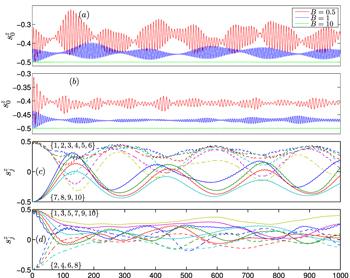
Figure 1. Time evolution of the spin polarization of individual spins, obtained from equation ( |
For models with short-range interactions, it is well-known that the time-evolution of non-equilibrium states is characterized by a light-cone dynamics of local observables [42–45]. On the other hand, the Gaudin magnets is a long-range model and, as shown in figures 1(c) and (d), the spin polarization of the bath spins evolve simultaneously into their steady-state value. Being infinite-range, the interaction of the Gaudin magnet can take effect without any propagation time.
Comparing the two initial states, we see that with ∣ΦA⟩ the bath spins need a much longer time than ∣ΦB⟩ to evolve into a steady state. In fact, for the initial state ∣ΦA⟩ the two groups of bath spins remain well distinct, and the oscillation in the spin polarization nearly approach periodically their initial values (1/2 or −1/2). On the other hand, the polarizations for the initial state ∣ΦB⟩ show an initial quick decay, leading to oscillations around 0. The evolution for the initial state ∣ΦA⟩ displays a strong memory of the initial domain-wall order. In order to further understand such peculiar dynamics, in later sections we will study the time evolution of the spin–spin correlations and the Loschmidt echo.
If the time-average $\bar{{ \mathcal O }}$ of an observable coincides with its micro-canonical ensemble average, i.e. $\bar{{ \mathcal O }}=\langle { \mathcal O }\rangle $ , the system reaches thermalization. Here the time average of the spin distribution ${\bar{s}}_{j}^{z}(t)=1/t{\int }_{0}^{t}{s}_{j}^{z}(\tau ){\rm{d}}\tau $ can be simply obtained from equation (8 ), by replacing $\cos ({w}_{{{kk}}^{{\prime} }}t)$ with $\mathrm{sinc}({w}_{{{kk}}^{{\prime} }}t)=\sin ({w}_{{{kk}}^{{\prime} }}t)/{w}_{{{kk}}^{{\prime} }}t$ . We see in figure 2(a) that the time-average of spin polarization of the central spin converges to clearly different values for the two initial states. The difference in the steady-state spin polarizations does not decrease by increasing N, see figure 2(b), in which smaller values of N(red circles) are obtained by exact method, relatively larger values of N(blue diamond) are obtained by MPS method. The combined results of BA and MPS method verify the persistence of a finite difference ${\bar{s}}_{0,A}^{z}-{\bar{s}}_{0,B}^{z}$ for the steady-state value. This observation confirms a breakdown of thermalization in the inhomogeneous central spin model, due to the restricted time evolution implied by integrability. Since the existence of conserved quantities, like ${H}_{j}=B{{\boldsymbol{s}}}_{j}^{z}+{\sum }_{k\ne j}{{\boldsymbol{s}}}_{j}\cdot {{\boldsymbol{s}}}_{k}/({\epsilon }_{j}-{\epsilon }_{k})$ , the time-evolution cannot be ergodic, neither in the whole Hilbert space nor in a subspace with fixed M.
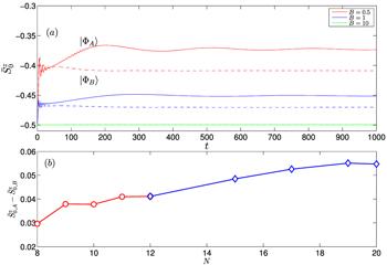
Figure 2. (a) Time average of the central spin polarization, computed for different values of B and N = 10. The solid lines are for the initial state ∣ΦA⟩ while the dashed lines are for the initial state ∣ΦB⟩. (b) Dependence of |
4. Spin–spin correlations
The spin–spin correlation function is defined as ${G}_{{mn}}^{z}(t)\,=\langle \psi (t)| {s}_{m}^{z}{s}_{n}^{z}| \psi (t)\rangle $ and, as discussed in appendix B , which can be computed in a way similar to the spin density. The explicit expression reads:
$\begin{eqnarray}\displaystyle \begin{array}{l}{G}_{{mn}}^{z}(t)=\sum _{k,k^{\prime} }\sum _{{j}_{1}\lt \cdots \lt {j}_{M}}\left(\displaystyle \frac{1}{2}-\sum _{\alpha =1}^{M}{\delta }_{{{mj}}_{\alpha }}\right)\left(\displaystyle \frac{1}{2}-\sum _{\alpha =1}^{M}{\delta }_{{{nj}}_{\alpha }}\right)\\ \quad \times \sum _{{ \mathcal P },{ \mathcal Q }}\displaystyle \frac{| {N}_{{\nu }_{k}}{| }^{2}}{\prod _{\alpha =1}^{M}({\nu }_{\alpha ,k}-{\epsilon }_{{{ \mathcal P }}_{\alpha }})({\nu }_{\alpha ,k}-{\epsilon }_{{{ \mathcal Q }}_{\alpha }})}\\ \quad \times \sum _{{ \mathcal P },{ \mathcal Q }}\displaystyle \frac{| {N}_{{\nu }_{k^{\prime} }}{| }^{2}}{\prod _{\alpha =1}^{M}({\nu }_{\alpha ,k^{\prime} }-{\epsilon }_{{{ \mathcal P }}_{\alpha }})({\nu }_{\alpha ,k^{\prime} }-{\epsilon }_{{{ \mathcal Q }}_{\alpha }})}\cos ({w}_{{{kk}}^{{\prime} }}t),\end{array}\end{eqnarray}$
which characterizes longitudinal correlation between spins.In figure 3, we show the spin–spin correlation function at different times, both for the initial state ∣ΦA⟩ (left panels) and ∣ΦB⟩ (right panels). On a relatively short timescale (t < 50), the correlation function is very similar to t = 0 for both initial states and when the evolution time approaches t ∼ 102 the correlation function has decreased to smaller values. However, it can be noted that in the left panels of figure 3 (referring to ∣ΦA⟩), the domain-wall order has not faded away completely even after a long evolution time t ∼ 103. This is in contrast to panel (h) on the right side, where the anti-ferromagnetic alignment has nearly disappeared. This confirms our previous observation that the domain-wall configuration is more favourable to retain memory of the initial state (see also figure 5 for the Loschmidt echo).
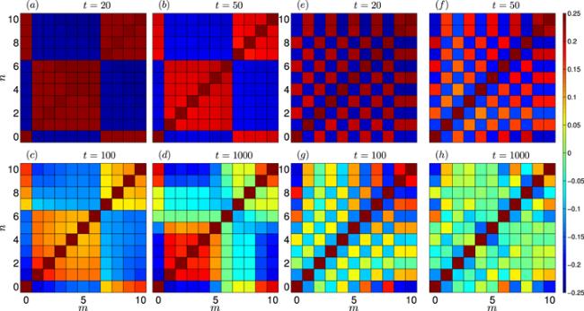
Figure 3. Left panels: the spin–spin correlation function |
From the contour plot of the correlations in figure 3, the correlations between the bath spins Gmnz with m, n > 0 tend to zero. Meanwhile the correlations between the central spin and bath spins ${G}_{m0}^{z}$ with m > 0 oscillate near initial value. After long enough time evolution (t ∼ 103), the correlations between the bath spins almost evolve toward to zero for the state ∣ΦB⟩.
Considering in more detail the right side of figure 3, we see in panel (g) that the correlations Gmnz with m, n ≳ 5 are more robust, and also the values of ${G}_{0n}^{z}$ with larger n remain rather similar to the initial values. This behavior is a consequence of the small coupling strength Aj when j is large, which implies a longer timescale for those bath spins. However, after a sufficiently long time evolution (t ∼ 103) the correlations between all spins are close to zero. The vanishing of correlations in panel (h) indicates that the steady state is like a paramagnetic state.
To further analyze the evolution of ${G}_{{mn}}^{z}(t)$ , we characterize the typical correlation strength for spin m as${\rm{\Delta }}{T}_{m}\propto -\mathrm{ln}t$ . In this interval the linear decay shown in figure 4 (on a semi-logarithmic scale) has its steepest slope. Finally, in the long-time limit the central spin is strongly entangled with bath spins and the value of Tm reaches its steady-state value. Due to finite-size effects, the decay is modified by oscillations, see especially panel (b), but the qualitative form and timescales are quite robust with respect to the value of m and the type of initial state.
$\begin{eqnarray}{T}_{m}=\sqrt{\displaystyle \frac{\sum _{n\ne m}{({G}_{{mn}}^{z}(t))}^{2}}{N}},\end{eqnarray}$
where the self-correlation terms Gmmz are excluded. In figure 4, we show the absolute value of correlation function and the typical correlation strength for the two initial states, i.e. the left two panels (a), (c) are for the initial state ∣ΦA⟩ and the right two panels (b), (d) for ∣ΦB⟩. For both ferromagnetic and anti-ferromagnetic alignment, the correlation strength decays from initial maximum value of 1/4 towards smaller values, with Tm = 0 corresponding to disordered spin alignment. We can see that there are two stages in the relaxation of correlations. After the initial decay (up to t ≲ 10, see the first black dash line), there is an intermediate regime in which the correlation strength has a logarithmic relaxation (up to t ∼ 102, near the second black dash line), i.e. 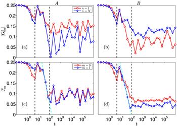
Figure 4. Panels (a) and (b) plot the spin–spin correlation function |
5. Loschmidt echo and MPS approach
The Loschmidt echo, defined as L(t) = ∣⟨Φ0∣ψ(t)⟩∣2, quantifies the memory of the initial state [46], thus can provide us a clear understanding of the difference between the evolution for the two initial states. By using equation (5 ), we express L(t) as:6 ). Finally, we obtain:
$\begin{eqnarray}L(t)=\sum _{k}\sum _{{k}^{{\prime} }}| \langle {{\rm{\Phi }}}_{0}| {\phi }_{k}\rangle {| }^{2}| \langle {\phi }_{{k}^{{\prime} }}| {{\rm{\Phi }}}_{0}\rangle {| }^{2}{{\rm{e}}}^{-{\rm{i}}{w}_{{{kk}}^{{\prime} }}t},\end{eqnarray}$
where the overlaps are given in equation ( $\begin{eqnarray}\displaystyle \begin{array}{l}L(t)=\sum _{k}\sum _{{k}^{{\prime} }}{\left[\sum _{{ \mathcal P }}\displaystyle \frac{| {N}_{{\nu }_{k}}| }{\prod _{\alpha =1}^{M}({\nu }_{\alpha ,k}-{\epsilon }_{{{ \mathcal P }}_{\alpha }})}\right]}^{2}\\ \quad \times {\left[\sum _{{ \mathcal P }}\displaystyle \frac{| {N}_{{\nu }_{{k}^{{\prime} }}}| }{\prod _{\alpha =1}^{M}({\nu }_{\alpha ,{k}^{{\prime} }}-{\epsilon }_{{{ \mathcal P }}_{\alpha }})}\right]}^{2}\cos ({w}_{{{kk}}^{{\prime} }}t).\end{array}\end{eqnarray}$
We show representative examples of the Loschmidt echo in figure 5. As seen in panel (a), for a weak magnetic field (B ∼ 0.5) the initial state ∣ΦA⟩ leads to a long-time evolution with large oscillations around a mean value $\bar{L}(t)\sim 0.25$ . Instead, panel (b) shows that L(t) ∼ 0 in the long-time limit, thus the system nearly loses its memory of the initial state ∣ΦB⟩.
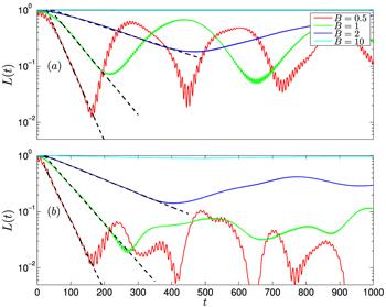
Figure 5. Time dependence of the Loschmidt echo for two different initial state. Panel (a) with the initial state ∣ΦA⟩, and panel (b) with initial state ∣ΦB⟩. |
In the first part of the time evolution, besides the presence of fast small amplitude oscillations, the Loschmidt echo displays a clear exponential dependence ${\rm{\Delta }}L(t)\propto \exp (-\gamma t)$ , up to an intermediate time scale t ∼ 102. According to our numerical calculation, the decay coefficients are similar for both initial states, i.e. γA ≃ γB ∼ 0.03 with B = 0.5. Such exponential scaling behavior of the Loschmidt echo has been widely found in dynamical evolution of quantum many-body system [47–50].
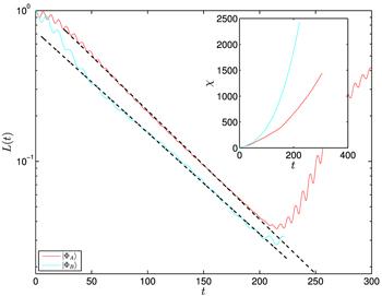
In order to confirm the scaling relaxation behavior of Loschmidt echo for a larger system size, we further perform an approximate calculation based on the MPS method [51, 52], as implemented in the Itensor library [53]. There are two important input parameters of the MPS simulations: the variational tolerance ε of the MPS wavefunction, which represents the error of the MPS state in approximating the true wavefunction (we use ε = 10−9 in our simulations), and the bond dimension χ, which indicates the maximum dimension of the matrices entering the variational ansatz. In the given implementation of the MPS method, the bond dimension is automatically increased to meet the desired tolerance. In figure 6, we show the Loschmidt echo for a bath size N = 50 and the two types of initial states considered in this work, ∣ΦA⟩ (red lines) and ∣ΦB⟩ (cyan lines). Also in this case the Loschmidt echo is characterized by an initial exponential decay, and this behavior persists up to intermediate times (t ≈ 102).
Figure 6. Loschmidt echo as function of time t for two different initial states by using an MPS method with N = 50. The red line is for the initial states ∣ΦA⟩, and the cyan line is for the initial state ∣ΦB⟩. |
Unfortunately, we are not able to access the long-time dynamics at N = 50 based on the MPS approach, as the entanglement in the wavefunction grows with time. This reflects itself on a rapid increase of the bond dimension χ, which eventually reaches numerically intractable values. The time dependence of χ in the simulation of figure 6 is shown in the inset. As seen, the bond dimension χ of initial state ∣ΦB⟩ grows faster in time than ∣ΦA⟩. Nevertheless, the range of times we can simulate is sufficient to establish conclusively the initial exponential form of decay of Loschmidt echo. In classical systems, the exponential decay of Loschmidt echo usually implies chaotic dynamics [49, 54, 55]. For the central spin model, the exponential decay of Loschmidt echo may indicate the dynamics is chaotic here as well [56].
6. Conclusion
In summary, based on Bethe Anstaz techniques, we have analytically studied the time evolution of several dynamic quantities of Gaudin magnets with arbitrary number M of flipped-down spins, such as spin distribution function, spin–spin correlation function, and Loschmidt echo. Furthermore, we have numerically studied the scaling behavior of the relaxation dynamics, up to relatively large system sizes. Significantly, the correlation function relaxes to its steady value with a logarithmic dependence, and the Loschmidt echo reveals an exponential loss of the memory of the initial state. Our results highlight several interesting features of the dynamical evolution of a quantum many-body system with long range interactions, thus advancing the understanding of decoherence for single qubits coupled to a spin bath at the many-body level. With respect to universal features of quantum many-body systems, much effort is still necessary to better understand the non-equilibrium quantum dynamics [57]. In future studies, it would be desirable to extend our methods to investigate scrambling in many-body system [58, 59], and the out-of-time-of-correlation function (OTOC) [60] of central-spin models. The details of such dynamical evolution of spin correlations may be accessible experimentally, e.g. through NMR techniques [61].